Functors and Computations in Floer homology with Applications Part II

(1)

Functors and Computations in Floer homology with Applications

Part II

C. VITERBO

^∗

October 15, 1996,

(revised on October 16, 2003)

Abstract

The results in this paper concern computations of Floer cohomology using generating functions. The first part proves the isomorphism between Floer cohomology and Generating function cohomology introduced by Lisa Traynor. The second part proves that the Floer cohomology of the cotangent bundle (in the sense of Part I), is isomorphic to the cohomology of the loop space of the base. This has many consequences, some of which were given in Part I, others will be given in forthcoming papers. The results in this paper had been announced (with indications of proof) in a talk at the ICM 94 in Z¨urich.

1 Introduction

This paper is concerned with computations of Floer cohomology using generating functions. The first part proves the isomorphism between Floer cohomology and Generating function cohomology introduced by Lisa Traynor in [Tr]. The statement of this theorem was given in [V2] with rather precise indications of proof. However, since then, we found what we consider a simpler, even though less natural, proof. A proof along the original indications is given by Milinkovi´c and Oh in [Mi-O1], [Mi-O2]. The second part proves that the Floer cohomology of the cotangent bundle (in the sense of Part I), is isomorphic to the cohomology of the loop space of the base. This has many consequences, some of which were given in Part I, others will be given in forthcoming papers.

We would like to point out a very interesting attempt by Joachim Weber to prove the main theorem of section 3 using a different approach, namely by considering the gradient flow of the geodesic energy as a singular perturbation of the Floer flow (see [We]).

2 Floer cohomology is isomorphic to GF-homology

Let L be a Lagrange submanifold in T^∗N, and assume L has a generating function quadratic at infinity, that is

L={(x,∂S

∂x)| ∂S

∂ξ(x, ξ) = 0}

where S is a smooth function onN×R^k, such thatS(x, ξ) coincides outside a compact set with a nondegenerate quadratic form in the fibers, Q(ξ). In particular if N is non-compact, L coincides with the zero section outside a compact set.

As proved by Laudenbach and Sikorav (see [LS]) this is the case for L= φ1(ON), where φt is a Hamiltonian flow.

Moreover S is ”essentially unique” up to addition of a quadratic form in new variables and conjugation by a fiber preserving diffeomorphism (the

”fibers” are those of the projection N ×R^k →N) see [V1] and [Th].

We may then consider, for L0 and L1 generated by S0, S1, the Floer cohomology F H^∗(L0, L1;a, b) of the chain complexC^∗(L0, L1;a, b) generated

(4)

by the points, x, in L0∩L1 with A(x)∈[a, b] where A(γ) isR

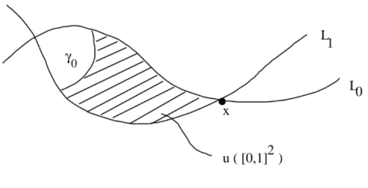
[0,1]²u^∗ω where u: [0,1]² →T^∗N is a map as in figure 1 such that

u(0, t) =γ0(t) u(s,0)∈L0

u(1, t) =γ(t) u(s,1)∈L1

where γ0 is a fixed path connecting L0 to L1, and x is identified with the constant path γx, at x.

Denoting byC^k the subvector space generated by the intersection points of L with the zero section having Conley-Zehnder index k, we have a differential:

δ:C^k(L0, L1;a, b)→C^k+1(L0, L1;a, b)

is obtained by counting the number of holomorphic strips, that are solutions of ¯∂u = ^∂u_∂s +J^∂u_∂t = 0 where J is an almost complex structure compatible with the symplectic form¹

u:R×[0,1]→ T^∗N u(s,0)∈L0 u(s,1)∈L1 S→±∞lim u(s, t) = x_±.

On the other hand, we have the much simpler space H^∗(S^b, S^a), where S(x, ξ, η) = S1(x, ξ)−S0(x, η), and S^λ = {(x, ξ, η) | S(x, ξ, η) ≤ λ}. This cohomology group does not depend on the choice of S according to [V1] and [Th], up to a shift in index, and was used in [Tr] as a substitute for Floer cohomology under the name GF cohomology (denoted GF^∗(L0, L1;a, b)).

Our first claim is Theorem 2.1.

F H^∗(L₀, L₁;a, b)≃GF^∗(L₀, L₁;a, b) The proof will take up the rest of this section.

Remark. : This was announced in [V2], together with a sketch of the proof.

Our present proof is actually simpler than the one we had in mind, in particular as far as the applications to the next section are concerned.

1i.e. ω(ξ, J ξ) defines a Riemannian metric

(5)

γ₀

x

L1

L0

u ( [0,1] ) 2

Figure 1: The map u.

We are first going to introduce a functional interpolating between A and S.

LetH(t, z, ξ) be a smooth function on R×T^∗N×R^k, equal to some non degenerate quadratic form Q(ξ) outside a compact set.

Forγ a path between L0 and L1, set AH(γ, ξ) =A(γ)−R1

0 H(t, γ(t), ξ)dt.

Set P(L0, L1) be the set of paths, γ, such that γ(0) ∈ L0, γ(1)∈ L1. Then the critical points of AH onP(L0, L1)×R^k are the pairs (γ, ξ) with

( .

γ −X_H(γ) = 0 R1

0

∂

∂ξH(t, γ(t), ξ)dt= 0

whereX_H is the Hamiltonian vector field associated to the function z → H(t, z, ξ) (i.e. ξ is ”frozen”).

If we denote byφ^t_ξ the Hamiltonian flow ofXH (for fixed ξ∈R^k) we have γ(t) =φ^t_ξ(γ(0)), so that the critical points of AH correspond to

{z ∈L0∩(φ^t_ξ)⁻¹(L1)|

Z 1 0

∂

∂ξH(t, φ^t_ξ(z), ξ)dt= 0}

Note that

LH ={φ¹_ξ(z)|z ∈L0, Z 1

0

∂

is an immersed Lagrange submanifold, and the above critical points correspond to LH ∩L0.

Consider an almost complex structure on M compatible with the symplectic form, and denote by ∂ = _∂s^∂ +J_∂t^∂.

(6)

We now define the Floer cohomology of AH as usual:

- C^∗ will be generated by the critical points of AH onP(L0, L1) - < d(x−, ξ−),(x+, ξ+)> equals the algebraic number of solutions of





u:R×[0,1]⇔M

∂u(s, t) = −∇H(t, u(s, t), ξ(s))

d

dsξ(s) =−R1 0

∂

∂ξH(t, u(s, t), ξ(s))dt satisfying lim

S→±∞(u(s, t), ξ(s)) = (x±, ξ±).

Note that the set of such solutions has its image in a bounded subset of T^∗N ×R^k.

Indeed, for u outside a bounded subset, H vanishes, so the equation becomes

( ∂u= 0

d

dsξ(s) =−R1 0

∂

∂ξH(t,0, ξ)dt

But the first equation cannot hold in the region foliated by pseudoconvex hypersurfaces.

If on the other hand |ξ| is large the equation will be ∂u=−∇H(t, u, ξ)

d

dsξ(s) =Bξ where Q(ξ) =< Bξ, ξ >.

But the second equation is such that any bounded set is contained in a set with the property that if a trajectory exits the set, it will never reenter it.

Thus, the set of bounded solutions has its image in a bounded set. Then the set of solutions satisfies the same formal properties as the set of solutions of the usual Floer equation. The proofs are just verbatim translations of those in [Fl1].

Definition. The cohomology of (C^∗(L0, L1, H), d) will be denoted byF H^∗(L0, L1, H).

If we restrict the complex to those solutions with AH(γ, ξ)∈[a, b] the cohomology is denoted F H^∗(L₀, L₁, H;a, b).

A first result is

(7)

Lemma 2.2. Let ψλ be a Hamiltonian flow on T^∗N, and Hλ , Fλ be the Hamiltonians with flows ψ⁻¹_λ ◦φ^t_ξ◦ψλ and φ^t_ξ◦(ψ^t_λ)⁻¹.

Then

F H^∗(L0, ψ1(L1), H0) =F H^∗(ψ₁⁻¹(L0), L1, H1) =F H^∗(L0, L1, F1) Proof. Consider first the chain complexC^∗(λ) = C^∗(ψ_λ⁻¹(L₀), ψ_λ⁻¹ψ₁(L₁), H_λ) for λ in [0,1]. It is generated by points in (ψ_λ⁻¹(L0))H_λ∩ψ_λ⁻¹ψ1(L1).

But (ψ⁻¹_λ (L0))Hλ is defined as {φ¹_λ,ξ(ψ⁻¹_λ (z))|z ∈L0;

Z 1 0

∂ξHλ(t, φ^t_λ,ξ(ψ⁻¹_λ (z)), ξ)dt= 0}

and sinceHλ(t, u, ξ) =H(t, ψλ(u), ξ) we haveHλ(t, φ^t_λ,ξ◦ψ_λ⁻¹(z), ξ) =H(t, φ^t_ξ(z), ξ) and φ^t_λ,ξ ◦ ψ_λ⁻¹ = ψ⁻¹_λ ◦φ^t_ξ, we have that (ψ⁻¹_λ (L0))H_λ = ψ⁻¹_λ ((L0)H) and ψ⁻¹_λ ((L0)H)∩ψ_λ⁻¹(ψ1(L1)) =ψ⁻¹_λ ((L0)H ∩ψ1(L1))

Thus the generators ofC^∗(λ) do not depend on λ.

Note also that the intersection points of (ψ_λ⁻¹(L0))Hλ and ψ⁻¹_λ (ψ1(L1)) stay transverse provided they are transverse for λ= 0 (that we shall always assume), and this is sufficient, together with the fact that the value of AH_λ

on the critical points does not depend on λ, to imply that the cohomology of C(λ) will not depend on λ.

Consider now the second equality. Note that we may deformH, provided its time one flow is unchanged, and the same for the flow ψλ.

We may thus assume that ∂_zH vanishes, (remember that H must be quadratic in ξ, hence it cannot vanish) for t in [0,²₃[, and Kλ, vanishes for t in [¹₃,1].

Then the flow (ψ_λ^t)⁻¹ ◦ φ^t_ξ is generated by H(t, ψ_λ^t(z), ξ) + K_λ(t, z) = Fλ(t, z, ξ) and therefore

∂ξFλ(t, z, ξ) = ∂ξH(t, ψ_λ^t(z), ξ) As a result,

(ψ_λ⁻¹(L0))H_λ = {φ¹_λ,ξ(ψ_λ⁻¹(z))|z ∈L0, Z 1

0

∂ξHλ(t, φ^t_λ,ξ◦ψ_λ⁻¹(z), ξ)dt= 0}

= {ψ_λ⁻¹φ¹_ξ(z)/z∈L0; Z 1

0

(8)

= {ψ_λ⁻¹φ¹_ξ(z)/z∈L0; Z 1

0

∂ξFλ(t,(ψ_λ^t)⁻¹◦φ^t_ξ(z), ξ)dt= 0}

= LF_λ

Thus we have

(ψ⁻¹_λ (L0))H_λ =ψ_λ⁻¹((L0)H) =LF_λ

andLFλ∩ψ⁻¹_λ ψ1(L1) is independent ofλ, and by the same argument as above, F H^∗(L0, ψ_λ⁻¹ψ1(L1), Fλ) does not depend on λ. Using again the invariance of the critical levels, we proved the second equality.

In particular forL₀ =O_N, L=φ₁(O_N) we get

F H^∗(ON, L,0) =F H^∗(ON, ON, H) Now let S(q, ξ) be a g.f.q.i. for L. The flow ofXS is given by

q˙= 0

˙

p= ^∂S_∂q(q, ξ) or

q(t)≡q(0)

p(t) =t_∂q^∂S(q, ξ) +p(0).

and (ON)S = {q,^∂S_∂q(q, ξ))|R1

0 ∂ξS(q(t), ξ)dt = 0} but since q(t) ≡ q(0), we have that R1

0 ∂ξS(q(t), ξ)dt = ∂ξS(q, ξ), hence (ON)S is the Lagrange submanifold generated by S.

Now we claim

Lemma 2.3. For S a g.f.q.i we have F H^∗(ON, ON, S;a, b)≃H^∗(S^b, S^a). Proof. Indeed the generators on both sides are critical points ofS, and connecting trajectories solve:

∂u=−∇qS(q(s, t), ξ(s))ds

d

dsξ(s) = −R1

0 ∂ξS(q(s, t), ξ(s))dt.

where u(s, t) = (q(s, t), p(s, t))

Now the function f(q, p) = |p| is pluri-subharmonic for our J, and since

∂u is tangent to kerdf (note that ∇_qS is horizontal), we have that f ◦u satisfies the maximum principle. Since p(s,1) = p(s,0) = 0, we must have p≡0, and thus

(9)

∂

∂sq(s, t) = −∇_qS(q(s, t), ξ(s))

∂

∂tq(s, t) = 0

In other words, q only depends on s, and satisfies q˙=−∇_qS(q(s), ξ(s))

ξ(s) =˙ −∂_ξS(q(s), ξ(s)) and lim

s→±∞(q(s), ξ(s)) = (q±, ξ±) are critical points for S.

Thus our connecting trajectories, are just bounded gradient trajectories for S, and thus the coboundary map is the same on both complexes, hence the cohomologies are the same.

We may finally conclude our proof. Let L = φ1(0N), so that it has a generating function S.

Now letSλ be the generating function ofLλ =φ⁻¹_λ (L), so thatS0 = 0 and S1 =S. We claim that the modulesF H^∗(Lλ,0N, Sλ, a, b) are all isomorphic.

Indeed, Lλ ∩ (0N)S_λ = φ⁻¹_λ (0N)∩ φ⁻¹_λ (L) = φ⁻¹_λ (0N ∩L) is constant and the usual argument proves the constancy of the Floer cohomology ring. It remains to show that

F H^∗(φ⁻¹₁ (0N),0N,0) =F H^∗(0N, φ1(0N),0) . Again this follows from the equality

F H^∗(φ⁻¹₁ (0N),0N,0) =F H^∗(φt◦φ⁻¹₁ (0N), φt(0N),0), becauseφtφ⁻¹₁ (0N)∩

φt(0N) =φt(φ⁻¹₁ (0N)∩0N).

We thus proved that

F H^∗(ON, L,0;a, b)≃F H^∗(ON, ON, S;a, b) Since

F H^∗(ON, L,0;a, b)≃F H^∗(L;a, b) and the above lemma proves states that

F H^∗(ON, ON, S;a, b)≃H^∗(S^b, S^a) =GH^∗(L;a, b) this concludes our proof.

(10)

3 The isomorphism of F H

^∗

( DT

^∗

N ) and H

^∗

(Λ N )

We will now compute F H^∗(M) for M =DT^∗N ={(q, p)∈ T^∗N | |p|g = 1}

for some metric g.

Let us denote by ΛN the free lopp space ofN (i.e. C⁰(S¹, N) ).

We have:

Theorem 3.1.

F H^∗(DT^∗N)≃H^∗(ΛN)

where ΛN is the free loop space of N. The same holds for S¹ equivariant cohomologies with rational coefficients.

The proof will take up the rest of this section. The next two lemmata are valid in any manifold satisfying the assumptions of section 2. First let us consider the diagonal ∆ in M×M, where M is the manifoldM endowed with the symplectic form −ω, and ϕ^t is the flow ofH onM.

Our first result is Lemma 3.2.

F H^∗(H;a, b)≃ F H^∗(∆,(Id×ϕ¹)∆;a, b).

Proof. Remember that F H^∗(H, a, b) =F H^∗(0,0, H, a, b).

We first point out that the cochain spaces associated to both sides are the same, and generated by the fixed points of ϕ¹.

The connecting trajectories are, for the left hand side given by

∂v =−∇H(t, v) v :R×S¹ →M

while for the right hand side, we first notice that F H^∗(∆,(id×ϕ¹)∆;a, b)≃ F H^∗(∆,(Id×ϕ¹)∆,0;a, b)≃ F H^∗(∆,∆,0⊕H;a, b) (Note: by K = 0⊕H we mean the Hamiltonian on M×M defined by K(t, z1, z2) =H(t, z2)).

The second isomorphism follows from lemma 2.2.

Now the coboundary map for this cohomology is obtained by counting solutions of

∂u=−∇K

where u= (u1, u2) :R×S¹ ⇔M ×M and ∂u1 = 0; ∂u2 =−∇H(t, u2).

(11)

Moreover, sincet→u(s, t) connects ∆ to itself, we haveu1(s,0) =u2(s,0) and u1(s,1) = u2(s,1).

Therefore we may glue togetheru1andu2to obtain a mapev :S¹×R→M such that

∂ev =−∇H(t,e ev)

where H(t, u) = 0 fore t in [0,1]

= H(t, u) for t in [1,2]

(the circle being identified with R/2Z). We shall make the simplifying as- sumption that H(t, z) = 0 for t close to 0 or 1, so that ˜H is continuous in t.

This is of course not a restriction on the time one map.

But the time 2 map ofHe coincides with the time 1 map forH, hence we may continuously deform one equation into the other, and the two cohomologies are isomorphic. (Rememeber that if we have a family of Hamiltonians depending continuously on some parameter, but having the same time 1 map, then the corresponding Floer cohomologies are alos independnt from the parameter).

Assumeϕ¹is equal toψ^r. We denote by Γϕthe graph ofϕ(i.e. Γφ= (id×

ϕ)∆), and Γ^ρ,r_ψ ={(z₁, ψ(z₂), z₂, ψ(z₃). . . , z_k−1, ψ(z_r), z_r, ψ(z₁))}in (M×M)^r Set ∆^r = ∆× ×∆ (r times)

Lemma 3.3. . For ϕ =ψ^r we have

F H^∗(∆,Γϕ;a, b)≃F H^∗(∆^r,Γ^ρ,r_ψ ;a, b)

Proof. Clearly, we may identify Γϕ∩∆ and ∆^r ∩Γ^ρ,r_ψ , since a point in this intersection is given by (z1, ψ(z2), . . . zr, ψ(z1)) = (z1, z1, . . . zr, zr) that is z1 =ψ(z2);z2 =ψ(z3), . . . , zr =ψ(z1) or else

z₁ =ψ^r(z₁), z_i =ψ^r+1−i(z₁) for i≥2

Note that there is a Z/r action on the set of such points, induced by z →ψ(z) on Γϕ∩∆ and by the shift (zj)→ (zj−1) on Γ^ρ,r_ψ ∩∆^r, and these two actions obviously coincide. We shall not mention this point in the proof, but all our results hold for Z/r equivariant cohomology with any coefficient

(12)

ring, and this eventually allows us to recover theS¹ equivariant cohomology (with rational coefficients), due to the Lemma in appendix 2 of [V3].

Now let us compare the trajectories.

For the second cohomology (uj, vj) :R×[0,1]→M satisfying





∂uj =∂vj = 0

uj(s,0) =vj(s,0) = 0 uj(s,1) =ψ(vj(s,1)) If we set w_j(s, t) =ψ_t(v_j(s, t)) so that





∂wj =∇K(s, t) ∂uj = 0 uj(s,0) =wj(s,0)

uj(s,1) =wj+1(s,1)

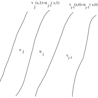
We may now glue together the uj and wj as in figure 2 to get a map u:R×R/2rZ→M

such that

u(s, t) = uj(s, t−2j) for 2j ≤t ≤2j + 1 u(s, t) = wj(s, t−2j−1) for 2j + 1≤t <2j+ 2 It satisfies ∂u=∇F(u) where

F(t, u) = K(t−2j, u) for 2j ≤t≤2j+ 1

= 0 otherwise

Thus the time 2k map of XF is equal toψ^k =ϕ.

We thus identified the Floer trajectories definingF H^∗(∆,Γ^ρ,r_ψ ;a, b) with those defining

F H^∗(H;a, b)≃F H^∗(∆,Γϕ;a, b) This concludes our proof.

Let us now prove theorem 3.1. LetHbe a Hamiltonian equal toH(t, q, p) = c|p| for |p| large, where cis some constant (that differs from the length of a closed geodesic, but will eventually become large), and ϕ^t its flow.

(13)

j-1 u

v (s,1)=u ( s,1) j j-1

j

vj-1

v (s,0)=u ( s,0)

j-1 j-1

v

j

Figure 2: The glueing of the maps uj and vj

(14)

For some integer r (that will eventually become large) set ψ = ϕ^1/r, so that ψ^r =ϕ¹ =ϕ.

Then according to lemmata 3.2 and 3.3, we have that F H^∗(H;a, b)≃F H^∗(∆^r,Γ^ρ,r_ψ ;a, b)

Now we may assume that H(t, q, p) = h(|p|) with h increasing and convex, and k is the Legendre dual of h. Let q(t) be a loop in M, and E(q) = R

S¹k(|q|)dt. Then we claim˙

F H^∗(H;a, b)≃H^∗(E^b, E^a)

We know from [V3] that there is a subset Ur,ε in ∆^r, defined by U_r,ε={(q_j, Pj)j∈Z/rZ|d(q_j, qj+1)≤ε/2}

for ε small enough, independent from r, such that Γ^ρ,r_ψ (that is ΓΦ in the notation of [V3]) is the graph of dSΦ over Ur,ε.

From proposition 1.8 in [V3], we have that there is a pseudogradient vector field ξΦ of SΦ such that, denoting by HI^∗ the cohomological Conley index (see [Co]), we have, for some integer d,

HI^∗(S_Φ^b, S_Φ^a;ξΦ)≃H^∗−d(E_r^b, E_r^a) where

E_r^b ={q= (qj)∈N^r|d(q_j, qj+1)≤ε/2 and Er(q)< b}

(Note: in [V3], E_r^b is denoted Λ^b_r,ε)

(Er(q) = sup_PSΦ(q, P) and dis some normalizing constant (equal in fact to rn).

On the other hand E_r^b ≃ E^b where E^b = {q ∈ ΛM|E(q) ≤ b} (see e.g.

[Mi]), so we only need:

Lemma 3.4.

F H^∗(∆^r,Γ^ρ,r_ψ ;a, b)≃HI^∗+d(S_Φ^b, S_Φ^a, ξΦ)

Proof. We would like to find an almost complex structureJ =J0, on (T^∗N× T^∗N)^r such that the holomorphic maps corresponding to Floer trajectories are also in one to one correspondence with bounded trajectories of ξΦ.

(15)

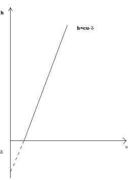
δ u h

h=cu-δ

Figure 3: The hamiltonian h

We first choose h so that the critical values of SΦ are in [−δ,0]. Indeed, we may impose that h^′(u)u−h(u) is in [−δ,0] (see Figure 3).

Then the Floer trajectories used to define the left hand side will have area less than 2δ.

Now, let us show that for δ small enough, such a Floer trajectory must stay inside T^∗Ur,ε0.

Indeed, since all critical points are inside T^∗(Ur,ε0/2), we have, for a Floer trajectory exiting from T^∗U_r,ε0/2, that it defines a J-holomorphic curve Σ such that

(i)

∂Σ⊂∆^r∪Γ^ρ,r_Φ . (ii)

Σ is in T^∗(Ur,ε0 − Ur,ε0/2).

Now we are in the following abstract situation:

LetV0 ⊂ V1 be convex sets, L0, L1 be disjoint Lagrange submanifolds in T^∗(V1 −V0). We set St =∂Vt = {x ∈ V1 | (1−t)d(x, V0) = td(x, V1)}, and Bt=∂T^∗Vt=T_S^∗_tV.

(16)

Let Σ be a holomorphic curve with boundary in L0∪L1. Then we claim that the area of Σ is bounded from below.

First let us consider the case of a pseudo-holomorphic curve, Σ closed in T^∗(V1 −V0) (and in particular with boundary in T_S^∗₀V ∪T_S^∗₁V ), such that

∂Σ∩T_S^∗0V =∂Σ∩B0 is non-empty.

ThenB1/2 must intersect Σ, since otherwise, as∂Σ∩B0 6=∅, there would be an interior tangency between some Bt (for 0< t < 1/2) and Σ, and this is impossible by the pseudoconvexity of Bt.

Thus for α = ¹₂d(V0, V1), and x0 ∈ B1/2∩Σ we have that B(x0, α) is in T^∗(V1−V0), and thus, we have

area(Σ)≥area(Σ∩B(x0, α)≥πα²exp(η(cα))

where c is an upper bound for the sectional curvatures of the metric g0

associated to ω and J (see Appendix).

Now consider the case where Σ has a boundary contained in the union of the two Lagrange submanifolds L0, L1.

LetU0, U1 be tubular neighbourhoods ofL0, L1 respectively, and assume that they are disjoint, symmetric (i.e. there is an anti-holomorphic diffeomorphism of Ui, fixing Li), and pseudoconvex. This can be easily achieved, through a perturbation of J near the Li.

Consider now ∂Σ∩L_i = γ_i. Then either γ₀ and γ₁ are both contained inside B1/2 or one of them is not.

In the first case, consider Σ∩T^∗(V1−V1/2). Then this intersection does not have a boundary in T^∗(V₁−V_1/2), except onB_1/2∪B₁, and we thus have again a lower bound on the area of Σ as in the case of a closed curve, except that α is to be replaced by α/2.

In the second case, assume for instance thatB1/2 intersects γ0.

Let us then consider the symetrization of Σ inside U0, where J is inte- grable, (see for instance [Si]). This will be a closed curve Σ inb U0, that has a point x0 in B1/2, and we also have a ball B(x0, α) in U0∩T^∗(V1−V0) for α ≤ inf{¹₂d(V0, V1),¹₂d(L0, ∂U0)}, and again, we get a lower estimate of the area of Σ. Since area(Σ)b ≥1/2 area(Σ), we also get an estimate on the areab of Σ.

This proves our abstract statement. We now claim that we are in the above framework, with α≃ε0/4.

Indeed, the diameter ofT^∗(U_r,ε− U_r,ε/2) isε/2, and we have to show that

∆^r has a pseudoconvex symmetric neighbourhood of radius ε/4.

(17)

But we will show that

(ii) Γ^ρ,r_Φ ∩T^∗(U_r,ε0 − U_r,ε0/2)∩ {|X_j| ≤ε0/4|Y_j| ≤ε0/4}=∅.

This implies that {|X_j| ≤ ε/4|Y_j| ≤ ε/4} is a tubular neighbourhood of the zero section, is disjoint from Γ^ρ,r_Φ in the region we are considering. Thus we have our U0, with radiusε/4. A similar fact would hold for Γ^ρ,r_Φ .

Let us now prove our last claim.

Indeed we only have to show that|^∂S_∂P^Φ

j| ≥ε/4 for (q, P) in Ur,ε0− U_r,ε0/2. But ^∂S_∂P^Φ

j ≃ q_j+1 −q_j − ¹_r^∂H_∂p +η(q_j+1 − q_j, P_j) (see [V3], proof of 1.2) where η(0, P) =dη(0, P) = 0, and since for some j, d(qj+1, qj)≥ ^ε₂, we have

|X_j|=|_∂P^∂S

j| ≥ ^ε₂ −^C_r ≥ ^ε₄⁰ forr large enough.

It is particularly important to notice that our lower bounds are independent from r, since they only depend on an upper bound for the sectional curvatures of the metric, and this quantity stays bounded as r goes to infinity.

If we choose δ < ¹₄ε we get that all Floer trajectories for J₀ must stay in T^∗Ur,ε0.

We claim that

(i) for a suitable choice ofJ1, theJ1 holomorphic curves defining the Floer cohomology are in one to one correspondence with trajectories of SΦ.

(ii) there is a family Jλ of almost complex structures connecting J0 to J1, taming ω and making T_∂U^∗ _r,ε0U_r,ε0 pseudo convex. Note that our almost complex structures will be time dependent, but this is not important.

Lemma 3.5. Let U be a manifold with boundary, and f : U → R be a smooth function. Then for L =graph(df), φt the Hamiltonian flow (q, p)→ (q, p+tdf(q)), set J(t, u) = (φt)∗J0(u).

Then, there is a one to one correspondence between solutions of ( q(t) =˙ −∇f(q(t))

s→±∞lim q(t) =x±

and







∂Jv = 0

v(s,0)∈0_N , v(s,1)∈L

s→±∞lim v(s, t) =x±

(18)

Proof. We have, setting v(s, t) =φtu(s, t)

∂Jv =dφt(u)∂

∂su(s, t) +J(∂

∂tφt)(u)

=dφt(u)[∂

∂t +dφt(u)[ ∂

∂S +dφ⁻¹_t (φt(u))Jdφt(u)∂

∂tu +∇H(u)]

=dφt(u)[∂J⁰u+∇H(u)

=dφt(u)[∂J0u+∇H(u)].

Thus

∂J0u=−∇H(u)

u(S,0)∈OU u(s,1)∈OU.

Now since H(q, p) = f(q), ∇H(q, p) = ∇f(q), and in local coordinates, we have dpj· ∇f(q) = 0.

Hence d(|p|)· ∂J⁰u = _|p|¹ Xn

j=1

dpj · ∇f(q) = 0 and |p ◦ u| satisfies the maximum principle. But since u(s,0)∈OU,u(s,1)∈OU, we havep◦u≡0, hence u(s, t) = q(s, t),0). Now ^∂q_∂t + _∂S^∂p = 0 is the second half of ∂_J0u =

−∇H(u), hence q(s, t) = q(t), and the first half becomes ˙q(t) =−∇f(q).

Note that if J0 makes T_∂U^∗ U pseudoconvex, the same holds for Jλ the linear interpolation between J₀ and J₁.

From this lemma, and the previous arguments, we may conclude that F H^∗(∆^k,Γ^σ,k_ψ ;a, b) is isomorphic to the cohomology of the Thom-Smale- Witten complex of ∇S_Φ restricted toS_Φ^b −S_Φ^a.

According to [Fl3] this last cohomology equalsHI^∗(S_Φ^b, S_Φ^a;∇SΦ).

Our proof will be complete if we are able to show that HI^∗(S_Φ^b, S_Φ^a;∇S_Φ)≃HI^∗(S_Φ^b, S_Φ^a;ξΦ)

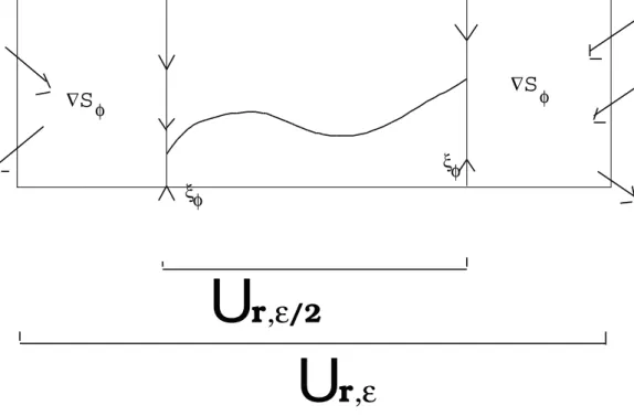
where ξΦ is as in [V3]. This may be explained by looking at figure 4.

We represented there a pseudogradient vector fieldηforSΦ, equal to∇SΦ

in a neighbourhood of Ur,ε− Ur,2ε/3 and toξΦ in a neighbourhood of Ur,ε/2.

(19)

ξφ ξφ

∇

S

∇

S

_φ φ

U ^r ^,ε U ^r ^,ε ^/2

Figure 4: The phase portrait of the pseudo-gradient ξΦ of SΦ

Now, all critical points ofSΦare insideU_r,ε/2, and a heteroclinic trajectory for η stays inside U_r,ε/2 since η=ξΦ on∂U_r,ε/2 is tangent to ∂U_r,ε/2.

Thus I^∗(U_r,ε, η)≃I^∗(U_r,ε/2, η).

But I^∗(Ur,ε, η)≃I^∗(Ur,ε,∇SΦ) sinceη =∇SΦ near ∂Ur,ε, and I^∗(U_r,ε/2, η)≃I^∗(U_r,ε/2, ξΦ).

Therefore

I^∗(Ur,ε,∇SΦ)≃I^∗(Ur,ε/2, ξΦ)

and our argument obviously extends if we restrict ourselves toS_Φ^b −S_Φâ. Thus I^∗(S_Φ^b, S_Φâ,∇S_Φ)≃I^∗(S_Φ^b, S_Φâ, ξΦ).

Note that these indices do not depend on ε, for r large enough, hence it is not important that the previous inequality relates the index of U_r,ε to the index of Ur,ε/2.

(20)

4 Appendix

Let (M, ω) be a symplectic manifold with contact type boundary, andJ0 be an admissible almost complex structure on M.

Given U a domain in M, and x0 in U, we consider wJ⁰,x⁰(U) = inf{

Z

C

ω |C isJ0- holomorphic, x0 ∈C}

and w(U), the usual Gromov width, is then given by

w(U) = sup{w_J0,x⁰(U)|x₀ ∈U, J₀ is admissible } A natural question is to compute the limits

k→+∞lim w(U^k) =w(U)

k→+∞lim wJ⁰,x⁰(U^k) = wJ⁰,x⁰(U)

Here we still denote by J₀ the almost complex structureJ₀×. . .×J₀ onM^k, and by x0 the point (x0, . . . , x0) in M^k.

Note that the sequence wJ⁰,x⁰(U) is obviously decreasing.

On the other hand, w(U) is not, a priori, equal to sup {w_J0,x⁰(U)|x₀ ∈ U, J0is admissible}=w(Ue ) since there are many more almost complex structures on M^k than those of the type J0 ×. . .×J0. Clearly, we have w(Ue )≤ w(U).

While it is clear, ifU contains a symplectic ball of radiusr, thatw(U)≥ πr², no such lower bound holds for wJ⁰,x⁰(U).

In fact, it is not a priori obvious thatw_J0,x⁰(U) is non zero. This is what we prove in this appendix.

Proposition 4.1. Let g0 be the metric associated to (ω, J0). Then, if the sectional curvature of g₀ is bounded byc, and injectivity radius at x₀ bounded by ρ, we have

wJ⁰,x⁰(U)≥πρ²δ(c, ρ)

where δ(c, ρ) is a continuous positive function, such that δ(c,0) = 1.

Lemma 4.2. LetBg0(r)be the ball of radiusr, centered atx0, for the metric g0. Let C be a minimal surface for g0 through x0. Then

area(C∩Bg (r))≥πr²exp(η(cr))

(21)

where η is continuous, η(0) = 0, and c is the upper bound of the sectional curvature of g0.

Proof. It is similar to the case where g0 is the euclidean metric. Set a(r) = area (C∩Bg0(r))

then a^′(r) = length(C ∩∂Bg⁰(r)) and since C is minimal, a(r) must be less than the area of the cone through x0, spanned by C∩∂Bg0(r).

Let us then compute the area of such a cone. It is clearly given by Rr

0 length(γs)ds where γs(t) = exp(^s_r ·exp⁻¹(cr(t))) and cr(t) is the curve C∩∂Bg0(r), the exponential being taken atx0.

Let M be a bound on the sectional curvature of g0. Then we have, by classical comparison theorems ([Pan] p.117, remark 8.14b)

kDexp_x0(u)k ≤ sinh(Mr)

Mr for kuk ≤r kDexp⁻¹_x₀(y)k ≤ Mr

sin(Mr) for y∈B(x₀, r) Thus

length (γs)≤ s r

sinh(Mr)

sin(Mr) ·length(Cr)

and Z r

0

length (γ_s)ds≤ r 2

sinh(Mr)

sin(Mr) ·length(Cr) and we have

a(r)≤ r

2ϕ(Mr)a^′(r) so that

a^′(r)

a(r) ≥ 2

rϕ(Mr) log(a(r)

a(ε)) ≥ logr² ε² +

Z r ε

2

uϕ(Mu)(1−ϕ(Mu))du

≥ log(r² ε²) +

Z M r M ε

21−ϕ(v)) vϕ(v) dr

(22)

Since 1−ϕ(u)∼uasugoes to zero, the quantity RM r M ε

2

u(ϕ(u))(1−ϕ(u))du converges to η(Mr) as ε goes to zero, with η continuous and η(0) = 0.

Then, since lim

ε→0

a(ε)

ε² ≥π, we have a(r)≥πr²exp(η(Mr)).

Now, replacing U by U^k, the sectional curvature of the induced metrics stays bounded (even though the bound may change as we go from k = 1 to k = 2), and since U^k contains (Bg0(ρ))^k, we get

ωJ⁰,x⁰(U^k)≥πρ²δ(c, ρ).

(23)

References

[Co] C.C. Conley,C.C.. Isolated Invariant Sets and their Morse Index.

C.B.M.S. Reg. Conf. Series in Math. n^o38, Amer. Math. Soc., Prov- idence,R.I., 1978.

[Fl1] A. Floer. The unregularized gradient flow of the symplectic action.

Comm. Pure and Appl. Math., 41:775–813, 1988.

[Fl3] A. Floer. Witten’s complex and Infinite dimensional Morse theory.

J. Differential Geometry, 30:207–221, 1988.

[LS] F. Lalonde and J.C. Sikorav. Sous-variétés lagrangiennes et lagrangiennes exactes des fibrés cotangents. Comment. Math. Helvetici, 66:18–33, 1991.

[Mi] J. Milnor. The h-cobordism theorem. Princeton University Press, Princeton, N.J. 1961.

[Mi-O1] D. Milinkovic and Y.G. Oh. Generating functions versus action functional preprint, University of Wisconsin, Madison

[Mi-O2] D. Milinkovic and Y.G. Oh. Floer homology as the stable Morse theory J. Korean Math. Soc.34:1065-1087, 1997.

[Pan] P. Pansu. Structures métriques pour les variétés riemanniennes Cedic, Fernand Nathan,Paris 1983 (english edition in preparation).

[Si] N. Sibony. Quelques probl`emes de prolongement de courants en analyse complexe. Duke Math. Journal., 52:157–197, 1985.

[Th] D. Th´eret PhD dissertation University of Paris 7 1995.

[Tr] L. Traynor Generating Function homology Geometry and Funct.

Analysis 4:718-748 1994.

[V1] C. Viterbo. Symplectic topology as the geometry of generating functions Math. Annalen, 692: 537-547, 1992.

[V2] C. Viterbo. Generating functions, Symplectic Geometry and Ap- plications. Proceedings of the ICM, Z¨urich, 94 Birkh¨auser Verlag, Basel.

(24)

[V3] C. Viterbo. Exact Lagrange submanifolds, periodic orbits and the cohomology of free loops spaces. J. of Differential Geometry. to appear.

[We] J. Weber. PhD dissertation TUB Berlin, in preparation

Functors and Computations in Floer homology with Applications Part II