Labour market returns of bachelor’s and master’s degrees in Germany: Differences and long-term developments

(1)

Labour market returns of bachelor’s and master’s degrees in Germany:

Differences and long-term developments

Johannes Wieschke, Maike Reimer, Susanne Falk

Dieser Artikel analysiert und vergleicht die längerfristigen Arbeitsmarkterträge von Bachelor- und Masterabsolventinnen und -absolventen in einem humankapital- theoretischen Kontext. Random-Effects-Panelregressionen zeigen, dass allgemein Personen mit Masterabschluss beim Berufseinstieg keine höheren Löhne erzielen, aber ihre Einkünfte rascher steigen. Dieses Muster findet sich unterschiedlich aus- geprägt in den meisten Fächern. Vor allem in den Ingenieur- und Naturwissenschaften liegt dies auch daran, dass an ein Masterstudium oft eine Promotion angeschlossen wird. Die längere Studiendauer von Masterabsolventinnen und -absolventen verschafft Bachelorabsolventen und -absolventinnen einen Vorsprung in Bezug auf die kumulierten Einkünfte, und erst nach einigen Jahren auf dem Arbeitsmarkt wird dieser Vorsprung geringer. Zumindest finanziell kann ein Masterabschluss daher auch als Investition betrachtet werden, die sich womöglich erst langfristig auszahlt.

1 Introduction

Since 1998, when Germany, France, Italy and the United Kingdom signed the Sorbonne declaration (Sorbonne Joint Declaration 1998), one-staged Diplom and Magister degrees have gradually been replaced by the two-tier bachelor’s and master’s degrees^. Due to the relative recency of the reform, the consequences of entering the labour market with either a bachelor’s or, some years later, a master’s degree have only begun to be investigated for labour market outcomes, especially income. Available studies relying on graduate surveys usually compare reported incomes at labour market entry (e. g. Bittmann, 2019; Glauser et al., 2019; Neugebauer & Weiss, 2018). Size and speed of subsequent income development, however, contribute substantially to overall benefits of educational attainment (Fuller, 2008). Bachelor programmes equate to full-fledged degrees preparing graduates for academic jobs, although they are shorter than the previous study programmes (KMK, 2003; Witte et al., 2008). The subsequent master’s degrees, usually taking another two years, focus on more advanced and abstract reasoning, research and leadership oriented skills. While completing a master’s degree can be seen as valuable investment in career advantages, it requires roughly another two years of education, thus postponing a regular income and reducing the earnings that can be accumulated over an extended period of time. Therefore, higher wages for master’s graduates do not necessarily result in an overall better economic

(2)

position due to the income advantage that bachelor’s graduates gain by their earlier labour market entrance. It also has to be considered that during this time, bachelor’s graduates already have the opportunity to acquire job-specific skills and training in work contexts, which also may increase their incomes and accelerate their income growth.

So far, little is known about absolute or relative income developments of graduates with either a bachelor’s or a master’s degree, or the factors that drive them. In this paper, we therefore address three analytical questions:

1. How do bachelor’s and master’s graduates differ with regard to entry level wages, wage development and cumulative returns for up to eight years after graduation?

2. How does time spent in employment affect labour market returns for the two degree types, and how does the time that some spend in a master’s programme compare to the time spent in employment with respect to labour market payoff?

3. All dimensions of income can be affected by characteristics of the graduates themselves (such as gender or grades), their university education (such as field of study or university type) and their labour market contexts (such as branch or entry level positions). What factors are driving differences in income levels and developments between bachelor’s and master’s graduates?

In chapter 2.1 we discuss relevant theoretical and conceptual ideas. In chapter 2.2 we outline national and international findings. Chapter 3 contains a description of the data used and the model variables. Results are presented in chapter 4, and in chapter 5, we draw conclusions and outline the limitations of our analyses.

2 Higher education and labour market outcomes 2.1 Theoretical perspectives

According to human capital theory, wages are determined by an individual’s productivity. The more productive someone is, the more valuable they are for an employer who can reward this with higher wages. Productivity can be increased in different ways, with education as one of the most important ones: the greater the amount of school- ing, the higher the productivity (Becker, 1962, 25). Another productivity-enhancing factor is work experience, accumulated over time on the job (Becker, 1962, 10 ff.).

Because there is a trade-off between education and work experience – the longer someone spends in the education system, the later they can fully enter the labour market (Sloane et al., 1996) – it can be difficult to determine which decisions maxim- ise wages. Therefore, when comparing master’s and bachelor’s incomes, three sce- narios may unfold:

(3)

■ First, the additional education of a master’s degree may be equivalent to the work experience that can be gathered in the same amount of time in terms of the effects on human capital. In this scenario, a parallel wage development can be expected:

At their labour market entry, respondents with a master’s degree would earn more than bachelor’s graduates at their entry and about as much as bachelor’s graduates with two years of work experience, i. e. about as much as a peer from the same bachelor’s graduation cohort would earn at that point. There would thus be no financial incentive for a master’s degree and even a financial disadvantage because, when the whole career is considered, master’s graduates would have less time to earn money.

■ Second, only education may constitute a full-time investment in human capital, while when working, significant amounts of time are spent only applying one’s human capital without increasing it. This would lead to higher incomes of master’s graduates compared to bachelor’s graduates of the same bachelor’s graduation cohort (i. e. with more work experience). This would not, however, necessarily mean that a master’s degree pays off in the long-term, because the wage advantage would first have to compensate the income lead gained by earlier labour market entry.

■ Third, obtaining a master’s degree may be an investment in productivity-enhancing skills (Barone & van de Werfhorst, 2011), since master’s degrees explicitly aim at providing advanced scientific analytical or leadership-oriented skills. Then human capital would not only increase faster during master’s studies than on the labour market, resulting in higher entry level incomes, but master’s graduates would also profit more from the same amount of subsequent work experience than bachelor’s graduates, resulting in steeper income growth for those holding a master’s degree.

Again, the wage advantage still does not necessarily compensate the income lead gained by earlier labour market entry of bachelor’s graduates.

Which scenario actually holds true may depend on contextual factors. In German higher education, field of study and university type strongly influence labour market entry, occupational status and income itself (Bol & van de Werfhorst, 2011; Klein, 2016;

Leuze, 2007; Noelke et al., 2012). Since curricular orientations and opportunities for further study differ between university types (Müller & Wolbers, 2003) at universities of applied sciences, a much smaller percentage of bachelor’s graduates continue with a master’s degree even within the fields of study offered at both types (Fabian et al., 2016). Also, field of study must be considered: in universities the transition rates are extremely high in some fields of study, making a person who enters the labour market with a bachelor’s degree in these fields a rather striking exception (Fabian et al., 2016).

It is therefore plausible to assume that within different fields of study or depending on university type, income differences may be reduced or more pronounced. Conse-

(4)

quently, we will include field of study and university type in our models and also analyse differences within fields of study separately to see if patterns differ.

In addition, characteristics of labour market contexts are relevant, as not all entry level positions are open to graduates with bachelor’s and master’s degrees equally. Access to certain advantageous or well-paid positions depends on the degree (DiPrete et al., 2017; Weeden, 2002). Most visibly, in collective wage agreements, master’s and bachelor’s degrees are assigned to different wage groups at labour market entry (Neugebauer & Weiss, 2018). If such positions are also connected with better career development prospects, the differential placement could also enable master’s graduates to achieve higher wage growth and to gain higher lifetime incomes than bachelor’s graduates despite having initially less work experience. A special case are doctoral positions that are available almost exclusively to master’s graduates and are not, in general, particularly well paid relative to other available positions. Depending on whether and within which time frame a PhD leads to income growth, income differences between bachelor’s and master’s graduates may be affected in different ways.

2.2 Previous findings

For Germany, a master’s degree is connected to higher entry level earnings relative to a bachelor’s degree in all fields of study except for design and art (Neugebauer &

Weiss, 2018). Among bachelor’s graduates, there is also a significant general advantage for those who graduated from universities of applied sciences (Trennt, 2019), at least in business and computer sciences, although not in technical subjects or design and art (Neugebauer & Weiss, 2018). Bachelor’s graduates with better grades, both in school and in university, have a much higher probability to continue with a master’s degree. Also, graduates from academic families take up a master’s degree much more often, partly due to their different educational pathways and educational performance before their bachelor graduation (Lörz et al., 2015; Neugebauer & Weiss, 2018). Income advantages could partly reflect this selection of the more productive students into master programmes.

In Switzerland, wages of graduates of universities are lower on average than those of graduates of universities of applied sciences, and any master’s degree leads to significant advantages (Glauser et al., 2019). For the United States, which have a long- standing two-tier system, Kane and Rouse (1995) found similar returns for graduates attending college for two years and four years, respectively. Regarding master’s and bachelor’s degrees, analyses further differentiating between degree types found positive effects on wages for master’s graduates relative to bachelor’s graduates, for certain fields of study (Jaeger & Page, 1996). Furthermore, a graduate’s (e. g. master’s) degree was associated with higher wages relative to an undergraduate’s (bachelor’s)

(5)

degree in most fields of study in the US, with the exceptions of liberal arts, humanities, and architecture where there was no difference (Kim et al., 2015) – or even a disadvantage in the humanities (Altonji et al., 2016). For England and Wales, too, post- graduates (e. g. with a master’s degree) were found to receive significantly higher wages than first degree holders (Walker & Zhu, 2011). Also, apart from wages, Bol and van de Werfhorst (2011) found that master’s degree equivalent (“higher tertiary”) relative to bachelor’s degree equivalent (“first stage tertiary degrees”) lead to higher occupational status positions in fifteen European countries. For a number of Central and Eastern European countries, similar effects were found (Noelke et al., 2012).

However, many of the discussed studies are based on cross-sectional data and often use OLS regression models for estimating economic returns to higher education, partly also disregarding mid- and long-term developments of wage returns. Cross-sectional designs do not accurately reflect the long-term returns of different degrees or majors.

Only a few studies model wage returns longitudinally on an individual level.

3 Data and operationalisation

The data stem from the Bavarian Graduate Panel (Bayerisches Absolventenpanel – BAP) in which cohorts of graduates of the universities and the public universities of applied sciences in Bavaria are surveyed about 1 year, 6 years and 10 years after graduation. Participants report about their studies and give extensive information about all the employments they have had so far (including starting and ending dates), resulting in panel data with an accuracy of one month.

For the following analysis, we use the first two panel waves of the graduation cohort 2008–10.¹ Data was collected first in spring 2012 and again between June 2017 and March 2018. In the first survey, about 15,000 out of 41,000 graduates contacted in total participated (response rate 37.5 %). After the second survey (response rate 43.7 %), the sample consisted of 6,764 individuals. We excluded participants who had graduated with a degree other than bachelor’s or master’s (e. g. a traditional Diplom or Magister degree); who did not report any employment; who reported implausible earnings (hourly wages of either less than 5 or of at least 100 euros, monthly incomes

1 Bachelor’s and master’s graduates who graduated between 1st October 2008 and 30th September 2010.

(6)

of less than 400 euros²) and who had at least one missing value on one of the important variables, leaving 2,398 persons for analyses.

As dependent variable, we use the logarithmised gross hourly wage, generated from the monthly incomes, the yearly bonuses and the weekly real working hours reported by graduates.³ As central analytical variables, we include the highest degree type (bachelor’s vs. master’s) with which individuals finally enter the labour market.⁴ Other time-invariant independent variables, representing potential drivers for income differences, include academic background, i. e. at least one parent with tertiary education, gender, A-level grade, field of study, type of university and number of employer changes. As time-variant independent variables, we include work experience (in months), executive positions, type of organisation and contract, sector, company size, and doctoral studies. Detailed information about dependent and independent variables are given in section 4.1, table 1 and table 2.

4 Analysis

4.1 Descriptive statistics

Table 1 shows how bachelor’s and master’s graduates differ with respect to the time- constant independent variables, with stars in the last column indicating whether the differences are statistically significant. The percentage of men is higher among master’s graduates, which is probably (in part) due to the fact that men more often study math and sciences, fields of study in which it is more common to continue with a master’s degree. With regard to university type, master’s graduates are more often university leavers, indicating that master’s programmes are predominantly offered at universities.⁵ It also appears that graduates with an academic family background or better school grades tend to self-select into master’s programmes, while bachelor’s and master’s graduates only slightly differ with regard to their job mobility, i. e. in the frequency of employer changes.

2 As a robustness check, the analysis was repeated with the top and bottom 2 %/5 % of incomes excluded.

Results remain largely the same, but more top earners are excluded and the effects for a master’s degree or for a degree in law/economics decrease, since these groups are overrepresented among top earners (detailed results available on request).

3 Alternative analyses using the contractual working time are available on request.

4 The group of master’s graduates includes those who obtained a master’s degree before the first survey, and those who at first were sampled as bachelor’s graduates and then obtained a master’s degree between the first and second survey.

5 Universities of applied sciences do not, as the table seems to indicate, produce almost half of all bachelor’s graduates; they do, however, produce almost half of the bachelor’s graduates who do not continue with a master’s programme but enter the labour market directly.

(7)

Table 1: Time-constant sample characteristics. Percentages and means Bachelor Master Total

Gender: male 43.7 % 51.7 % 50.1 % **

University 44.5 % 78.0 % 71.3 % ***

Field of study

–Humanities 19.3 % 14.8 % 15.7 % *

–Social sciences 18.1 % 8.8 % 10.7 % ***

–Law and economics 30.1 % 26.0 % 26.8 %

–Math and sciences 18.1 % 31.9 % 29.1 % ***

–Engineering 14.3 % 18.5 % 17.7 % *

Academic background 46.4 % 58.2 % 55.8 % ***

School grade 2.33 2.05 2.11 ***

Ever employer change 44.1 % 49.8 % 48.6 % *

Number of employer changes 0.60 0.67 0.65

N (persons) 481 1,917 2,398

N (person months) 34,122 119,125 153,247

Source: BAP 2008–10, authors’ calculations; performed with Stata 15

Significance of difference between Bachelor and Master: * p < 0.05, ** p < 0.01, *** p < 0.001.

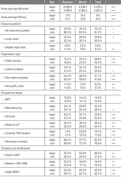
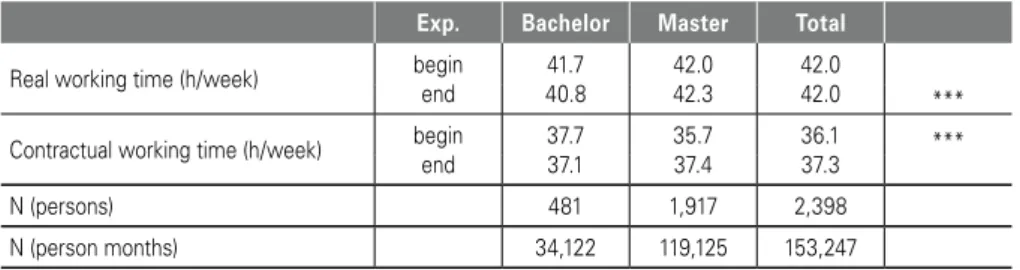
Table 2 shows how time-variant job characteristics differ between the two types of degree holders at the beginning and the end of the observation period (see column marked “Exp”). With regard to our dependent variables, master’s graduates earn significantly more. Their advantage is larger at the end of the observation period, both in absolute and relative terms, and amounts to 622 euros (per month) and 2.6 euros (per hour).

There is no such clear-cut advantage with regard to job or labour market characteristics.

Master’s graduates less often hold executive positions and less often have permanent contracts. While part of this may be due to fact that PhD positions occur almost exclusively among master’s graduates, many of these differences still hold up at the end of the observation period (when most PhDs are completed) and when PhD students are excluded (results available on request). Master’s graduates, especially in later career stages, are more frequently employed in large and/or listed companies (where wages tend to be higher), but also more often in the public service (where wages tend to be lower).

(8)

Table 2: Time-variant sample characteristics at the beginning and end of the observa- tion period. Percentages and means

Exp. Bachelor Master Total

Gross earnings (€/month) begin 3,036.9 3,336.4 3,276.3 ***

end 3,766.0 4,385.3 4,261.0 ***

Gross earnings (€/hour) begin 17.0 18.3 18.1 ***

end 21.2 23.8 23.3 ***

Executive position

–No executive position begin 70.9 % 76.4 % 75.3 % *

end 56.3 % 62.4 % 61.2 % *

–Lower level begin 24.5 % 20.0 % 20.9 % *

end 32.2 % 30.1 % 30.5 %

–Middle–high level begin 4.6 % 3.5 % 3.8 %

end 11.4 % 7.5 % 8.3 % **

Organisation type

–Public service begin 15.2 % 33.4 % 29.8 % ***

end 16.6 % 27.3 % 25.2 % ***

–Listed company begin 19.1 % 20.7 % 20.4 %

end 21.2 % 25.5 % 24.6 % *

–Non-listed company begin 54.3 % 38.5 % 41.7 % ***

end 50.5 % 39.6 % 41.8 % ***

–Non-profit, other begin 11.4 % 7.4 % 8.2 % **

end 11.6 % 7.5 % 8.3 % **

Occupational sector

–BIC^$ begin 15.6 % 14.2 % 14.5 %

end 14.8 % 13.1 % 13.4 %

–Manufacturing begin 24.1 % 25.8 % 25.4 %

end 24.7 % 30.4 % 29.2 % *

–Services begin 35.1 % 20.7 % 23.6 % ***

end 31.2 % 20.9 % 23.0 % ***

–Media et al.^# begin 25.2 % 39.4 % 36.5 % ***

end 29.3 % 35.6 % 34.4 % **

–Currently PhD student begin 1.9 % 23.8 % 19.4 % ***

end 1.2 % 13.5 % 11.0 % ***

–Permanent contract begin 80.2 % 57.7 % 62.3 % ***

end 89.8 % 73.7 % 76.9 % ***

Company size (employees)

–Small (<100) begin 43.2 % 34.8 % 36.5 % **

end 38.5 % 29.2 % 31.0 % ***

–Medium (100–499) begin 22.5 % 16.9 % 18.0 % **

end 22.9 % 17.1 % 18.3 % **

–Large (500+) begin 34.3 % 48.3 % 45.5 % ***

end 38.7 % 53.7 % 50.7 % ***

To be continued next page

(9)

Exp. Bachelor Master Total

Real working time (h/week) begin 41.7 42.0 42.0

end 40.8 42.3 42.0 ***

Contractual working time (h/week) begin 37.7 35.7 36.1 ***

end 37.1 37.4 37.3

N (persons) 481 1,917 2,398

N (person months) 34,122 119,125 153,247

Notes: ^$ BIC: banks, insurances, consulting; ^# Media et al.: Media, education, associations Significance of difference between Bachelor and Master: * p < 0.05, ** p < 0.01, *** p < 0.001.

4.2 Multivariate analysis

To examine our three research questions, we estimate a series of six random-effects panel regressions (where the effects of the time-constant degree variable can be measured) with the logarithmised hourly wages as the dependent variable (see table 3).

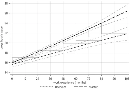
The first model includes only degree type and duration of work experience in months (linear, squared and interaction with degree) as independent variables, putting relative wage effects of degree type and work experience in direct comparison. Figure 1 shows the average marginal effects of this first model as rising curves. As can be seen, master’s graduates earn only slightly more than bachelor’s graduates at the beginning of their respective careers, and the difference gains significance only after several months. However, respondents with a master’s degree experience steeper wage growth, so that the gap between the earnings of those with a bachelor’s degree increases over time. The straight grey lines link master’s graduates’ wages with those of bachelor’s graduates with two more years of work experience (thus directly comparing roughly two years spent in education with two years of work experience). Initially, their work experience puts bachelor’s graduates at an advantage, but between two and three years after graduation, master’s graduates gain the lead.

Table 2 continued

(10)

Figure 1: Hourly wages of bachelor’s and master’s graduates. Model 1 without control variables. Average Marginal Effects with 95 % Confidence Intervals

14 16 18 20 22 24 26 28

gross hourly wage

0 12 24 36 48 60 72 84 96 108

work experience (months)

Bachelor Master

In models 2–6, we add additional independent variables (see table 3): In model 2, personal characteristics and study performance; in model 3, university type, field of study, and labour market sectors; in model 4, information about doctoral studies and the type of organisation; in model 5, further job characteristics, and in model 6, information about employer changes. The consequences of all model steps for the main effect (i. e. the income difference between degrees coefficient) are visualised in figure 2. The upper six lines represent the sizes of the degree coefficient, i. e. the wage difference between bachelor’s and master’s graduates when both have no work experience for all six models. The lower six lines represent the coefficient of the interaction of the degree with work experience, i. e. how much the wage difference grows with each year of work experience. The horizontal lines show the 95 % confidence intervals; where they cross the zero line, no significant effect is present.

(11)

Figure 2: Stepwise Random-Effects panel regressions of log. hourly wages. Coeffi- cients of main effects with 95 % Confidence Intervals

Master

Ma*exp (years)

−.05 0 .0 5 .1 .1 5

degree+exp. +gender, acad., A−level grade +subject, uni, sector +PhD, orga−type +contract, executive, comp. size +employer change

The main effect of the degree type, as can be seen in figure 2, is not significant at first, and this does not change when personal characteristics are included. However, the effect increases and becomes significant in model 3, when field of studies, type of university (university or university of applied sciences) including a degree interaction and occupational sector are included, and increases further when information about PhD studies and the type of organisation are added in model 4. Master’s graduates thus earn significantly more relative to bachelor’s graduates, once PhD students, who have lower wages on average, are controlled for. Adding information about employer changes affects the difference only slightly.

Regarding wage differences between the two different university types, the positive master effect is less pronounced for master’s graduates from universities who earn significantly less than master’s graduates from universities of applied sciences, as the negative interaction effect shows. This coefficient decreases and loses its significance after controlling for PhD students, who are overrepresented among graduates from universities. Differences between university types therefore seem to be mainly driven by field of study and PhD students.

(12)

Among the job characteristics added in model 5, several exert significant influence on respondents’ wages. For example, wages are higher in the manufacturing sector, in large companies, or for those with a permanent contract or an executive position.

However, there are no marked differences between bachelor’s and master’s graduates with regard to these variables – at least with PhD students already controlled for.

Therefore, neither the degree effect nor its interaction with work experience changes very much through inclusion of these labour market characteristics. The inclusion of the employer changes in model 6, however, diminishes the impact of work experience (only the squared variable is still significant after that), resulting in less steep wage growths.

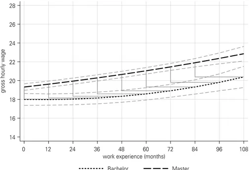
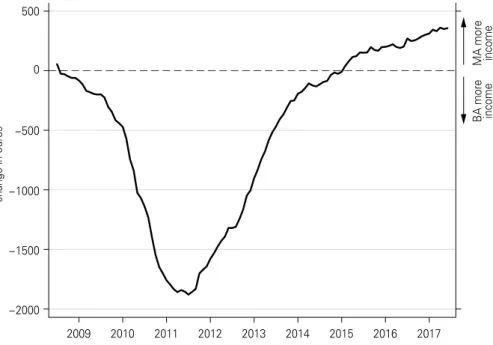
Figure 3 shows the average marginal effects of model 6, where all control variables are included. Already at labour market entry, master’s graduates have a wage advantage relative to bachelor’s graduates (even relative to those with more work experience), and their wage growth is still steeper.

Figure 3: Hourly wages of bachelor’s and master’s graduates. Model 6 with all control variables. Average Marginal Effects with 95 % Confidence Intervals

14 16 18 20 22 24 26 28

gross hourly wage

0 12 24 36 48 60 72 84 96 108

work experience (months)

Bachelor Master

(13)

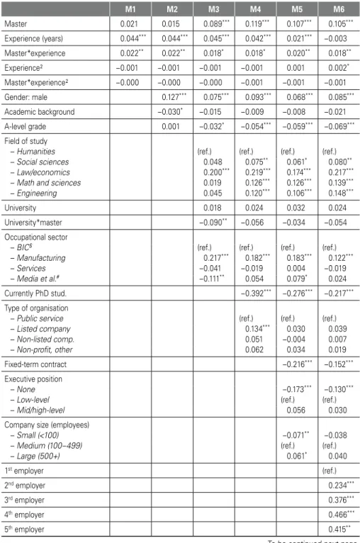
Table 3: Random-effects panel regressions of log. hourly wages

M1 M2 M3 M4 M5 M6

Master 0.021 0.015 0.089^*** 0.119^*** 0.107^*** 0.105^***

Experience (years) 0.044^*** 0.044^*** 0.045^*** 0.042^*** 0.021^*** –0.003 Master*experience 0.022^** 0.022^** 0.018^* 0.018^* 0.020^** 0.018^**

Experience² –0.001 –0.001 –0.001 –0.001 0.001 0.002^*

Master*experience² –0.000 –0.000 –0.000 –0.001 –0.001 –0.001

Gender: male 0.127^*** 0.075^*** 0.093^*** 0.068^*** 0.085^***

Academic background –0.030^* –0.015 –0.009 –0.008 –0.021

A-level grade 0.001 –0.032^* –0.054^*** –0.059^*** –0.069^***

Field of study

–Humanities (ref.) (ref.) (ref.) (ref.)

–Social sciences 0.048 0.075^** 0.061^* 0.080^**

–Law/economics 0.200^*** 0.219^*** 0.174^*** 0.217^***

–Math and sciences 0.019 0.126^*** 0.126^*** 0.139^***

–Engineering 0.045 0.120^*** 0.106^*** 0.148^***

University 0.018 0.024 0.032 0.024

University*master –0.090^** –0.056 –0.034 –0.054

Occupational sector

–BIC^$ (ref.) (ref.) (ref.) (ref.)

–Manufacturing 0.217^*** 0.182^*** 0.183^*** 0.122^***

–Services –0.041 –0.019 0.004 –0.019

–Media et al.^# –0.111^** 0.054 0.079^* 0.024

Currently PhD stud. –0.392^*** –0.276^*** –0.217^***

Type of organisation

–Public service (ref.) (ref.) (ref.)

–Listed company 0.134^*** 0.030 0.039

–Non-listed comp. 0.051 –0.004 0.007

–Non-profit, other 0.062 0.034 0.019

Fixed-term contract –0.216^*** –0.152^***

Executive position

–None –0.173^*** –0.130^***

–Low-level (ref.) (ref.)

–Mid/high-level 0.056 0.030

Company size (employees)

–Small (<100) –0.071^** –0.038

–Medium (100–499) (ref.) (ref.)

–Large (500+) 0.061^* 0.040

1^st employer (ref.)

2^nd employer 0.234^***

3^rd employer 0.376^***

4^th employer 0.466^***

5^th employer 0.415^**

To be continued next page

(14)

M1 M2 M3 M4 M5 M6 Constant 2.749^*** 2.704^*** 2.703^*** 2.607^*** 2.860^*** 2.839^***

N (persons) 2,398 2,398 2,398 2,398 2,398 2,398

N (person months) 153,247 153,247 153,247 153,247 153,247 153,247

R² (overall) 0.102 0.131 0.249 0.339 0.376 0.347

Notes: ^$ BIC: banks, insurances, consulting; ^# Media et al.: Media, education, associations

* p < 0.05, ** p < 0.01, *** p < 0.001.

To analyse whether these patterns hold true for all fields of study, we estimated separate regressions for all five fields of study included here (detailed results available on request). The analyses show that in model 1, when only degree type and work experience are included, there is a positive effect of master’s degree only within law and economics, while in math/sciences, the effect is negative. This is probably due to the differences in the share of PhD students in these two fields, which is very low in law and economics and very high in math and sciences. Eventually, however, the wages of master’s graduates in most fields of study surpass those of bachelor’s graduates with the same amount of work experience – the exception being the humanities.

For graduates of the humanities and social sciences, it is interesting to note that doctoral studies do not have a marked influence, because wages of PhD students do not differ significantly from those of others in these fields. This makes obtaining a doctoral degree a less risky additional investment in education for these graduates: A financial disadvantage accumulates during master’s studies, but not anymore after that, while for a master’s graduate in math/sciences the disadvantage will continue to rise if they choose to do a doctorate. Depending on the subject, PhD studies can therefore be seen as a long-term investment or as no true investment at all, because in some cases there are no opportunity costs associated with the decision to pursue a PhD.

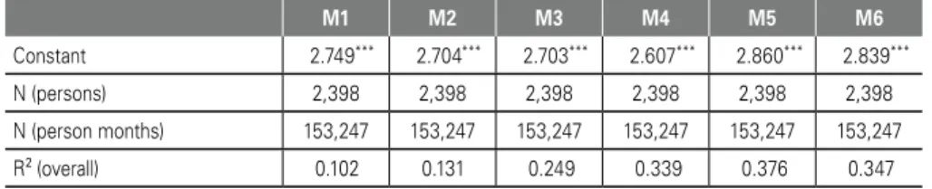
4.3 Cumulated incomes

In this section, we will investigate how bachelor’s and master’s incomes add up over time until the end of the observation period when respondents possess up to eight years of work experience. For this purpose, we only use bachelor’s graduates of the graduation cohort 2008–10 and compare those who did not proceed to complete a master’s degree with those who did.

Table 3 continued

(15)

Figure 4: Average cumulated gross monthly incomes. Bachelor’s graduation cohort 2008–10 with and without master’s studies afterwards

cumulated income (in thousand)

difference (in thousand) –60 –30 0 0

50 100 150 200 250

2009 2010 2011 2012 2013 2014 2015 2016 2017

no MA MA difference

Figure 4 shows the average cumulated gross monthly incomes of bachelor’s graduates with and without a further master’s degree above the zero line, and the difference (calculated as bachelor’s earnings minus master’s earnings) below the zero line.⁶ A rise in cumulated incomes can be observed from 2010 on for graduates without further studies, and from 2011 on for those with further studies, marking the points in time when significant numbers of graduates of these groups start to enter the labour market. The difference in average cumulated incomes meanwhile grows – indicated by the third line descending ever further into the negative area – until the year 2014, when masters lag more than 60,000 euros behind. In 2015, the difference starts to decrease – indicated by the line not descending any further and even slightly reversing at the end of the observation period – but still amounts to more than 50,000 euros around 2017.

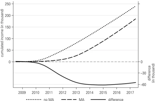
Figure 5 shows in detail how this difference develops over time. The descent of the line is most pronounced and most rapid in the first years until 2011, when the average graduate without further studies earns more than 1,500 euros more than the average graduate who proceeded to complete a master’s degree. This does not mark the point

6 If an employment was not observed in a particular month, the respondent was included with the value zero in the calculation of the average.

(16)

where the incomes of the first group are highest, but the point where most of them have already entered the labour market while many of the comparison group have not yet done so. After that, the line rises closer to zero again, indicating that the difference in cumulated incomes still rises, but not as fast anymore: The work experience-related wage gains by graduates without further studies are offset by the large income increases of the master’s graduates who just enter the labour market (and thus make jumps from zero to several thousand euros).

Figure 5: Change in cumulated income difference. Bachelor’s graduation cohort 2008–10 with vs. without master’s studies afterward

MA more income

BA more income

−2000

−1500

−1000

−500 0 500

change in euros

2009 2010 2011 2012 2013 2014 2015 2016 2017

However, as can be seen in figure 1, master’s graduates initially have a wage disadvantage compared to respondents of the same age but without further studies (i. e.

bachelor’s graduates who started working 24 months ago) due to a lack of work experience. Therefore, the cumulated wage difference only begins to decrease in 2015, as the steeper wage growth of master’s graduates compensates for the disadvantage in work experience. At least in the first two or three years afterward, the difference does not decrease as fast as it increased in the first years of the observation period, because bachelor’s graduates usually begin to work about two years earlier, and during this time their wages exceed those of the later master’s graduates (who at this point are mostly still master’s students) far more than master’s graduates’ wages later exceed those of bachelor’s graduates.

(17)

In the separate analyses for fields of study, some differences can be found (detailed results available on request). In math/sciences and in engineering, the cumulated income difference is still growing at the end of the observation period. In math/sciences, this is mainly the result of high numbers of PhD students who earn significantly less than other graduates who entered the labour market, with or without a master’s degree. In engineering, the mechanism is different: Engineers with a master’s degree initially do not earn more than those with just a bachelor’s degree and the same amount of work experience – again, mainly because of PhD students – but also, the returns to work experience only slightly differ. Therefore, engineers with a master’s degree cannot compensate the disadvantage in work experience with steeper income growth as effectively as master’s degrees in other fields of study. For other subjects, the difference in cumulated incomes decreases much faster, because doctoral studies do not exert such pronounced negative effects. Especially in the humanities the difference is also much smaller to begin with (less than 40,000 euros at its peak).

5 Discussion and conclusion

The aim of this study was to assess the effects of a master’s degree on entry wages, wage development and cumulative returns relative to that of a bachelor’s degree for a period of up to eight years after graduation with a longitudinal analysis of income levels and wage growth. We took into account that bachelor’s graduates have an earlier opportunity to achieve an income and to acquire relevant human capital in a working environment, and investigated which context factors associated with the person, their higher education and their labour market influence the differential returns.

Our results show that master’s graduates do not have significantly higher entry wages, contrary to expectations derived from human capital theory. Since they experience steeper wage growth, however, the additional human capital acquired in education seems to be of higher value than the work experience that can be obtained on the labour market in the same time, insomuch that incomes of master’s graduates eventually overtake those of bachelor’s graduates within the time period observed. These results thus expand the findings of Neugebauer and Weiss (2018) which showed income differences in early careers in general.

The master advantage seems to be partially driven by the fact that higher achieving students and men are more likely to take up a master’s degree and also to have higher incomes. On the side of the labour market, doctoral positions are especially important:

Because these positions are almost exclusively available to master’s graduates, and often have relatively low incomes, they lower the average wages of master’s graduates. When PhD students are controlled for, respondents with a master’s degree earn significantly more at labour market entry than those with a bachelor’s degree, and

(18)

experience even steeper wage growth, although important job characteristics like company size, the type of contract or executive positions are not always in their favour.

With respect to cumulative income, however, incomes of master’s graduates do not yet fully compensate the earlier gainful employment of bachelor’s graduates and their considerable wage growth through work experience. The estimations suggest that it may take several more years to make up for the delayed entry.

While the patterns remain similar in most fields of study, the field-specific prevalence and relative disadvantage of doctoral studies leads to variations. In math and sciences, doctoral studies are most common as well as more distinctly associated with lower wages relative to other job opportunities. In this field, therefore, the average entry wages of master’s graduates are significantly lower, and – just like in engineering – the lifetime earnings gap gets particularly large and for a long time does not begin to close.

In other subjects (especially in the humanities), where PhDs are less prevalent and/or relatively well paid, the gap does not get as big and closes faster. Thus, in some subjects, master’s and especially PhD studies have to be seen as a long-term investment with regard to financial outcomes.

One aspect that remains to be investigated more in depth is the role of the two university types. In our analyses, whether the master’s degree was acquired at a university or university of applied sciences does have an overall influence on wages, but this also depends on the control variables included in the models. Additional analyses should therefore focus on subpopulations which share the same degree, subject and university type.

A limitation of our study is the fact that respondents could not be followed over their whole career, primarily because the widespread introduction of the new bachelor’s and master’s degrees in Germany is still quite recent. Bachelor’s or master’s graduates may, in the long run, be more prone to employment interruptions, e. g. because of unemployment or parenthood, thus either widening or decreasing the gap. Moreover, it is quite plausible that the absence of a master’s degree can be disadvantageous, especially mid-career, when employees move up to managerial positions. It is yet unclear how many of the bachelor’s graduates will return to higher education later after some years of work experience in order to increase their labour market prospects.

The more extended the time period under scrutiny, the more important it will become to include general educational and labour market trends to accurately estimate relative advantages for master’s or bachelor’s degree holders.

When estimating cumulated incomes over longer periods of time, additional limitations have to be considered. Due to a later entry into the labour market, master’s graduates

(19)

overall tend to work less – although it is possible that their degree also decreases the likelihood of unemployment, resulting in similar amounts of work experience in the long run – but for higher wages. Because of progressive taxes, however, working two months for a gross income of 1,000 euros per month can result in a higher net income than working one month for 2,200 euros. On the other hand, in the second scenario higher entitlements e. g. to a pension are acquired. Master’s graduates may furthermore later, have to take on debts to finance their longer educational period. While the BAP contains some limited information on family structure and work regions, the information is not sufficient for an analysis of that kind.

Whether and how labour market returns of later graduation cohorts follow similar patterns cannot be answered with the data used. Since bachelor’s and master’s graduates entered the labour market at different points in time here, it is also possible that period effects assert some influence as well – indeed, in this sample the original master’s graduates have higher starting salaries than those who obtained their master’s degree later. Depending on the cohorts under investigation, the differences between bachelor’s and master’s graduates reported here could thus also be smaller or bigger.

Another limitation is the fact that the sample consists of persons with at least one university degree from Bavaria and is thus not representative of Germany as a whole in certain aspects. While the Bavarian higher education system is large and diverse, the labour market is decidedly better than average, and wages are on average higher than in the rest of Germany (Eichhorn et al., 2010). However, this affects bachelor’s graduates as well as master’s graduates, and the mechanisms analysed here are expected to be similar in all parts of Germany – after all, standardisation and compa- rability of higher education systems not only on a national level, but even in all of Europe were central goals of the Bologna reform.

References

Altonji, J.G., Arcidiacono, P. & Maurel, A. (2016): The analysis of field choice in college and graduate school: Determinants and wage effects. In Hanushek, E.A., Machin, S.

& Woessmann, L. (eds.), Handbook of the Economics of Education, vol. 5, 305–396 Barone, C. & van de Werfhorst, H.G. (2011): Education, cognitive skills and earnings in comparative perspective. International Sociology, 26(4), 483–502. https://doi.

org/10.1177/0268580910393045

Becker, G.S. (1962): Investment in Human Capital: A Theoretical Analysis. Journal of Political Economy, 70(5, Part 2), 9–49

Bittmann, F. (2019): Explaining the Mechanisms linking Field of Study and Labour Market Outcomes: Focus on STEM (Working Paper). OPUS. https://fis.uni-bamberg.

(20)

de/bitstream/uniba/45073/1/BittmannSTEMkorrse_A3b.pdf. Accessed 14 January 2020

Bol, T. & van de Werfhorst, H.G. (2011): Signals and closure by degrees. The education effect across 15 European countries. Research in Social Stratification and Mobility, 29(1), 119–132. https://doi.org/10.1016/j.rssm.2010.12.002

DiPrete, T.A., Eller, C.C., Bol, T. & van de Werfhorst, H.G. (2017): School-to-Work Linkages in the United States, Germany, and France. American Journal of Sociology, 122(6), 1869–1938. https://doi.org/10.1086/691327

Eichhorn, L., Huter, J. & Ebigt, S. (2010): Reiche und arme Regionen, Reichtum und Armut in den Regionen—zur sozialen Geographie Deutschlands. Statistische Monats- hefte Niedersachsen, 06, 286–304

Fabian, G., Hillmann, J., Trennt, F. & Briedis, K. (2016): Hochschulabschlüsse nach Bologna: Werdegänge der Bachelor- und Masterabsolvent(inn)en des Prüfungsjahr- gangs 2013. Forum Hochschule 2016,1. DZHW Deutsches Zentrum für Hochschul- und Wissenschaftsforschung, Hannover

Fuller, S. (2008): Job Mobility and Wage Trajectories for Men and Women in the United States. American Sociological Revue, 73(1), 158–183

Glauser, D., Zangger, C. & Becker, R. (2019): Aufnahme eines Masterstudiums und Renditen universitärer Hochschulabschlüsse in der Schweiz nach Einführung von Bologna. In Lörz, M. & Quast, H. (eds.), Bildungs- und Berufsverläufe mit Bachelor und Master, 17–52. Springer, Wiesbaden

Jaeger, D.A. & Page, M.E. (1996): Degrees Matter. New Evidence on Sheepskin Effects in the Returns to Education. The Review of Economics and Statistics, 78(4), 733–740. https://doi.org/10.2307/2109960

Kane, T.J., & Rouse, C.E. (1995): Labor-Market Returns to Two- and Four-Year College.

American Economic Review, 85(3), 600–614

Kim, C., Tamborini, C.R. & Sakamoto, A. (2015): Field of Study in College and Lifetime Earnings in the United States. Sociology of Eduation, 88(4), 320–339. https://doi.

org/10.1177/0038040715602132

Klein, M. (2016): The association between graduates’ field of study and occupational attainment in West Germany, 1980–2008. Journal for Labour Market Research, 49(1), 43–58. https://doi.org/10.1007/s12651-016-0201-5

Kultusministerkonferenz (KMK) (2003): Strukturvorgaben für die Einführung von Bach- elor-/Bakkalaureus- und Master-/Magisterstudiengängen. Beschluss der Kultusminis- terkonferenz vom 10.10.2003. https://www.kmk.org/fileadmin/pdf/PresseUndAk- tuelles/2003/strukvorgaben.pdf. Accessed 14 January 2020

Leuze, K. (2007): What Makes for a Good Start? Consequences of Occupation-Specific Higher Education for Career Mobility: Germany and Great Britain Compared. Interna- tional Journal of Sociology, 37(2), 29–53. https://doi.org/10.2753/IJS0020-7659370202

(21)

Lörz, M., Quast, H. & Roloff, J. (2015): Konsequenzen der Bologna-Reform: Warum bestehen auch am Übergang vom Bachelor- ins Masterstudium soziale Ungleichheiten?

Zeitschrift für Soziologie, 44(2), 137–155. https://doi.org/10.1515/zfsoz-2015-0206 Müller, W. & Wolbers, M.H. (2003): Educational attainment in the European Union:

recent trends in qualification patterns. In Müller, W. & Gangl, M. (eds.), Transitions from Education to Work in Europe: The Integration of Youth into EU Labour Markets, 23–62

Neugebauer, M. & Weiss, F. (2018): A Transition without Tradition. Earnings and Unemployment Risks of Academic versus Vocational Education after the Bologna Process. Zeitschrift für Soziologie, 47(5), 349–363. https://doi.org/10.1515/zfsoz-2018- 0122

Noelke, C., Gebel, M. & Kogan, I. (2012): Uniform Inequalities. Institutional Differen- tiation and the Transition from Higher Education to Work in Post-socialist Central and Eastern Europe. European Sociological Review, 28(6), 704–716. https://doi.org/10.1093/

esr/jcs008

Sloane, P.J., Battu, H. & Seaman, P.T. (1996): Overeducation and the formal education/

experience and training trade-off. Applied Economics Letters, 3(8), 511–515. https://

doi.org/10.1080/135048596356131

Sorbonne Joint Declaration (1998): http://www.ehea.info/media.ehea.info/file/1998_

Sorbonne/61/2/1998_Sorbonne_Declaration_English_552612.pdf. Accessed 14 Janu- ary 2020

Trennt, F. (2019): Zahlt sich ein Master aus? Einkommensunterschiede zwischen den neuen Bachelor-und Masterabschlüssen. In Lörz, M. & Quast, H. (eds.), Bildungs- und Berufsverläufe mit Bachelor und Master, 371–397. Springer, Wiesbaden

Walker, I., & Zhu, Y. (2011): Differences by degree. Evidence of the net financial rates of return to undergraduate study for England and Wales. Economics of Education Review, 30(6), 1177–1186. https://doi.org/10.1016/j.econedurev.2011.01.002

Weeden, K.A. (2002): Why Do Some Occupations Pay More than Others? Social Closure and Earnings Inequality in the United States. American Journal of Sociology, 108(1), 55–101. https://doi.org/10.1086/344121

Witte, J., van der Wende, M. & Huisman, J. (2008): Blurring Boundaries: How the Bologna Process Changes the Relationship between University and Non-University Higher Education in Germany, the Netherlands and France. Studies in Higher Education, 33(3), 217–231. https://doi.org/10.1080/03075070802049129

Manuskript eingereicht: 08.09.2020 Manuskript angenommen: 09.10.2020

(22)

Angaben zu den Autoren:

Dr. Johannes Wieschke Deutsches Jugendinstitut e. V.

Nockherstraße 2 81541 München E-Mail: wieschke@dji.de Dr. Maike Reimer

E-Mail: reimer@ihf.bayern.de Dr. Susanne Falk

E-Mail: falk@ihf.bayern.de

Bayerisches Staatsinstitut für Hochschulforschung und Hochschulplanung (IHF) Lazarettstraße 67

80636 München

Johannes Wieschke ist seit Oktober 2020 wissenschaftlicher Referent beim Deutschen Jugendinstitut in der Corona-KiTa-Studie. Von 2015 bis 2020 war er am Bayerischen Staatsinstitut für Hochschulforschung und Hochschulplanung in der Absolventen- forschung tätig und forschte vor allem zu Arbeitgeberwechseln und Einkommensent- wicklung.

Susanne Falk und Maike Reimer sind wissenschaftliche Referentinnen am Bayerischen Staatsinstitut für Hochschulforschung und Hochschulplanung (IHF). Susanne Falks Forschungsschwerpunkte sind Übergänge vom Studium in den Arbeitsmarkt, wissenschaftlicher Nachwuchs, Studienabbruch sowie internationale Studierende. Maike Reimers Arbeitsschwerpunkte sind Bildungs- und Berufsverläufe, fachliche Differenzierung sowie Kompetenzerwerb im Hochschulbereich.