Spatial Chow-Lin Models for Completing Growth Rates in Cross-sections

IHS Economics Series Working Paper 295

April 2013

Spatial Chow-Lin Models for Completing Growth Rates in Cross-

sections

Wolfgang Polasek

Impressum Author(s):

Wolfgang Polasek Title:

Spatial Chow-Lin Models for Completing Growth Rates in Cross-sections ISSN: Unspecified

2013 Institut für Höhere Studien - Institute for Advanced Studies (IHS) Josefstädter Straße 39, A-1080 Wien

E-Mail: o ce@ihs.ac.at ffi Web: ww w .ihs.ac. a t

All IHS Working Papers are available online: http://irihs. ihs. ac.at/view/ihs_series/

This paper is available for download without charge at:

https://irihs.ihs.ac.at/id/eprint/2195/

Spatial Chow-Lin Models for Completing Growth Rates in Cross-sections

Wolfgang Polasek

295

Reihe Ökonomie

Economics Series

295 Reihe Ökonomie Economics Series

Spatial Chow-Lin Models for Completing Growth Rates in Cross-sections

Wolfgang Polasek April 2013

Institut für Höhere Studien (IHS), Wien

Institute for Advanced Studies, Vienna

Contact:

Wolfgang Polasek

Department of Economics and Finance Institute for Advanced Studies Stumpergasse 56

1060 Vienna, AUSTRIA

: +43/1/599 91-155 email: polasek@ihs.ac.at and University of Porto Rua Campo Alegre Portugal

Founded in 1963 by two prominent Austrians living in exile – the sociologist Paul F. Lazarsfeld and the economist Oskar Morgenstern – with the financial support from the Ford Foundation, the Austrian Federal Ministry of Education and the City of Vienna, the Institute for Advanced Studies (IHS) is the first institution for postgraduate education and research in economics and the social sciences in Austria. The

Economics Series

presents research done at the Department of Economics and Finance and aims to share “work in progress” in a timely way before formal publication. As usual, authors bear full responsibility for the content of their contributions.

Das Institut für Höhere Studien (IHS) wurde im Jahr 1963 von zwei prominenten Exilösterreichern –

dem Soziologen Paul F. Lazarsfeld und dem Ökonomen Oskar Morgenstern – mit Hilfe der Ford-

Stiftung, des Österreichischen Bundesministeriums für Unterricht und der Stadt Wien gegründet und ist

somit die erste nachuniversitäre Lehr- und Forschungsstätte für die Sozial- und Wirtschafts-

wissenschaften in Österreich. Die

Reihe Ökonomie

bietet Einblick in die Forschungsarbeit der

Abteilung für Ökonomie und Finanzwirtschaft und verfolgt das Ziel, abteilungsinterne

Diskussionsbeiträge einer breiteren fachinternen Öffentlichkeit zugänglich zu machen. Die inhaltliche

Verantwortung für die veröffentlichten Beiträge liegt bei den Autoren und Autorinnen.

Abstract

Growth rate data that are collected incompletely in cross-sections is a quite frequent problem. Chow and Lin (1971) have developed a method for predicting unobserved disaggregated time series and we propose an extension of the procedure for completing cross-sectional growth rates similar to the spatial Chow-Lin method of Liano et al. (2009).

Disaggregated growth rates cannot be predicted directly and requires a system estimation of two Chow-Lin prediction models, where we compare classical and Bayesian estimation and prediction methods. We demonstrate the procedure for Spanish regional GDP growth rates between 2000 and 2004 at a NUTS-3 level. We evaluate the growth rate forecasts by accuracy criteria, because for the Spanish data-set we can compare the predicted with the observed values.

Keywords

Interpolation, missing disaggregated values in spatial econometrics, MCMC, Spatial Chow- Lin methods, predicting growth rates data, spatial autoregression (SAR), forecast evaluation, outliers

JEL Classification

C11, C15, C52, E17, R12

Comments

Preprint submitted to Elsevier.

Contents

1 Introduction 1

1.1 Eurostat and the regional data base for Europe ... 2

2 The Chow-Lin method for non-summable (intensive)

variables 3

2.1 The basic Chow-Lin method ... 3 2.2 Assumptions for the Chow-Lin forecasting procedure ... 5 2.3 Some properties of the Chow-Lin forecasts ... 5

3 The system Chow-Lin method for completing growth rates 7

3.1 The non-spatial intensive Chow-Lin procedure ... 7 3.2 The spatial extension of the system Chow-Lin (SAR-SCL) model ... 10 3.3 A two step feasible GLS (FGLS) estimation ... 14

4 A Bayesian Chow-Lin model for completing growth rates 15

4.1 The Bayesian Chow-Lin prediction of growth rates ... 17 4.2 Sampling a conditional r.v. from a joint distribution ... 19 4.3 Model selection by marginal likelihood ... 20

5 Application of the spatial Chow-Lin to Spanish regions 20 6 Outliers in the aggregate equation 22

7 Conclusions 23

8 References 24

9 APPENDIX: Higher order SAR models 25

9.1 MCM: Griddy Gibbs for the SARX model ... 25

9.2 The SAR(2) model ... 26

1. Introduction

Completing data sets at a disaggregated level when only aggregated values can be observed can be done by the Chow and Lin (1971) method. The original method was proposed for time series, but in Polasek and Sellner (2010) this method was extended for cross-sectional data based on a spatial autoregressive model, for panel data and for spatial flow models. An implicit assumption of the Chow-Lin approach is the summability of disaggregated variables to aggregated variables, a property that holds for so-called intensive variables. This paper shows how to extend the spatial Chow-Lin approach for cross-sectional data to non-extensive or inten- sive variables, like growth rates. In Physics ”an extensive variable is one that is additive for independent, non- interacting subsystems” (Wikipedia, Feb. 6th, 2013, http : //en.wikipedia.org/wiki/Extensive

q

uantity).

Many data are collected by Eurostat via the individual EU member states using common rules and methods. But not all member states have started at the same time their data collection, and therefore data series are often incomplete. In 1995 Eurostat introduced the harmonized European national accounting system. This leads to inhomogeneous data quality and sometimes to holes in the database if smaller regional units are needed. In order to apply many modern panel estimation methods one has to complete such data sets. While the simplest (deterministic) method to repair data holes is deterministic interpolation, this does not always give satisfactory results, and we prefer to use model based stochastic (imputation) methods for the missing disaggregated values.

For spatial data, this paper focuses on completing data sets that are growth rates or are extensive (i.e.

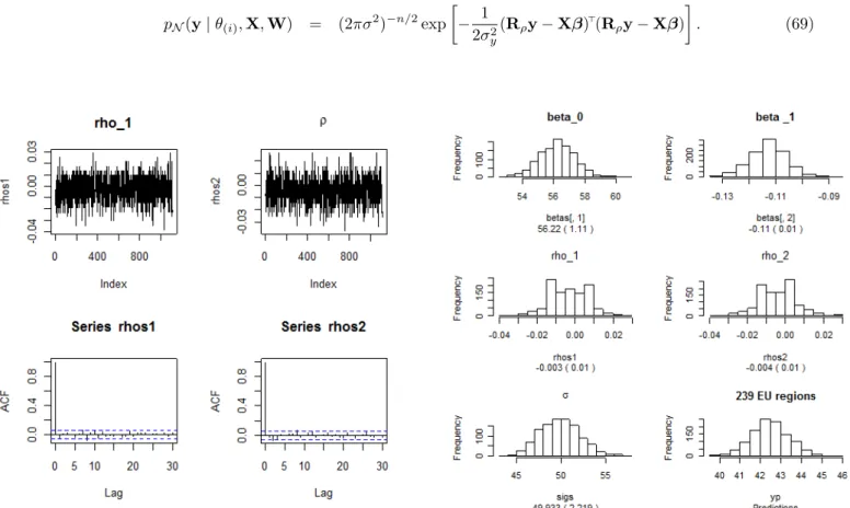
summable) cross-sectional variables and we discuss two extensions of the Chow and Lin (1971) method: We will use spatial econometrics (see e.g. Anselin (1988) ) and also the Bayesian MCMC approach as e.g. in LeSage and Pace (2009).

The paper is organized as follows. Section 2 outlines the classical estimation and prediction in the spatial

and non-spatial system Chow-Lin (CL) model. The classical (BLUE) estimator for the spatial autoregressive

model (SAR) is derived, along with the error covariance matrix needed for the improved prediction of the

missing values, which leads to the so-called spatial gain terms for predictions. Section 4 describes the

Bayesian approach for the spatial system Chow-Lin method together with the MCMC algorithms and

we show how the numerical predictive densities for the missing disaggregated values can be obtained by

simulating from the conditional density in the system approach. Furthermore we show that the method

can also be used in the presence of outliers in the system Chow-Lin model. An example for completing

the growth rates are given in section 5. We apply the spatial Chow-Lin method to Spanish NUTS-2 and

NUTS-3 data. Because for Spain we can observe all data on the disaggregated level, we will evaluate the

quality of the spatial Chow-Lin method by comparing the predicted values for GDP at the NUTS-3 level to their observed values and calculate the usual forecast accuracy criteria. A final section concludes.

1.1. Eurostat and the regional data base for Europe

Eurostat publishes regional data on a range of different statistical topics, collected by the 27 member states, but also from candidate countries and by the four EFTA states. Usually, this information is collected at different spatial levels based on the nomenclature of territorial units for statistics (NUTS).

NUTS data are collected by the individual member states using common rules and methods. However, not all member states have developed the same level and speed of skills, especially after 1995 when the harmonized European economic account system started. This can lead to inhomogeneous data quality and sometimes to holes in the data base, especially if it comes to smaller regional units where never had been data collected before. Thus, although in 2003 the NUTS system was acquired as a basis for a regional EU data base, it is common to find that the data at the lowest levels of disaggregation (NUTS-3) is missing for some countries and indicators. Moreover, periodical changes in the NUTS regulation occur since the regional classification adapts to the new administrative boundaries or economic circumstances. Consequently, these changes lead to additional disconnections in the time series, which can lead to breaks in the information at the lowest spatial units under consideration.

Sometimes it is difficult to obtain a complete set of panel data of all EU regions at the NUTS-3 level covering even the most basic indicators referred to demographics, labor markets, infrastructure, prices or productivity. For example, if one downloads the Eurostat information for regional GDP at the NUTS-3 level for the EU 27, including EFTA countries and EU candidate countries for the period 1995-2005, one would find that 15% of the numbers are missing. On top of that, the problems of data restriction at the NUTS-3 level increases for more disaggregated components of the regional accounts, either from the supply (Gross Value Added by industries), the demand (investments, public or public expenses) or the income side (salaries or capital remuneration). Finally, as it has been described above, it could also be the case that the right spatial level for analyzing a specific economic phenomenon requires the use of data even at a lower level of aggregation as the presently available NUTS-3 data.

LeSage and Pace (2004) use spatial econometric techniques to estimate missing dependent data. They predict unobserved house prices by using the information of sold and unsold houses to increase the estimation efficiency. LeSage and Pace (2004) predict unobserved spatially dependent data with observable data at the same regional level. The goal is to predict unobserved dependent variables for all regions.

2

2. The Chow-Lin method for non-summable (intensive) variables

Chow-Lin (1971) developed a method to forecast (”construct”) quarterly times series observations from yearly observations, by using appropriate ”indicators” or auxiliary regressors for the quarterly series. This approach can be extended for constructing disaggregated observations in the spatial context if only aggre- gated observations are available again using indicator variables in the forecasting equation, as it was shown in Polasek and Sellner (2010). As a basis for the subsequent analysis we first review the Chow-Lin method as proposed in Llano et al. (2009).

2.1. The basic Chow-Lin method

Disaggregate (or high frequency) time series are occasionally needed since they offer valuable information for policy makers. However, such data on a monthly or quarterly basis are often not available- for various reasons. Attempts have been made to interpolate missing high frequency data by using related series that are known. Friedman (1962) suggested relating the series in a linear regression framework. The three problems in connection of missing data are known by statisticians as interpolation, extrapolation and the distributional problem of time series by related series. Interpolation is used to generate higher frequency level (or stock) data, while extrapolation extends a given series outside the sample period, and in the distribution framework one allocates lower frequency flow data, such as GDP (see Fernandez, 1981), to higher frequency observations. The path-breaking paper by Chow and Lin (1971) embedded the missing data problem to a predictive system framework of aggregate and disaggregate data, leading to a boost in research on this topic.

We assume a linear relationship for the high frequency (disaggregate) data y

_d

and the indicators X

_d

, i.e.

y

_d

= X

_d

β

_d

+ ε

_d

with ε

_d

∼ N [0, σ

²

Ω], (1)

where y

d

is a (n × 1) vector of unobserved disaggregate variables, but X

d

is a (n × k) matrix of observed regressors. β

d

is a (k × 1) vector of regression coefficients, and ε

d

is a vector of random disturbances, with mean E (ε) = 0 and covariance matrix E (ε

d

ε

⁰_d

) = σ

²

Ω, Chow and Lin (1971) showed that the BLUE for the regression parameter ˆ β

d

and the disaggregated (or unobserved high frequency) data ˆ y

d

are given by

β ˆ

_d

= (X

_d⁰

C

⁰

(CΩC

⁰

)

⁻¹

CX

_d

)

⁻¹

X

_d⁰

C

⁰

(CΩC

⁰

)

⁻¹

y

_a

(2) ˆ

y

d

= X

d

β ˆ

d

+ ΩC

⁰

(CΩC

⁰

)

⁻¹

(y

a

− CX

d

β ˆ

d

), (3)

where y

_a

= Cy

_d

is the observed dependent variable at the aggregated level (while y

_d

is unobserved at the disaggregated level), and C is a N × n (with n ≥ N) aggregation matrix consisting of 0’s and 1’s, indicating which cells have to be aggregated together. The essential part in the equation 2 and 3 is the residual covariance matrix Ω, which has to be estimated. The Chow-Lin procedure for the BLUE requires the knowledge or assumptions about this error covariance matrix. In the literature assumptions like random walk, white noise, Markov random walk or autoregressive process of order one have been suggested and tested (e.g. Fernandez, 1981; Di Fonzo, 1990; Litterman, 1983; Pavia-Miralles et al., 2003). Some authors extended the framework for the multivariate case (e.g. Rossi, 1982; Di Fonzo, 1990) covering time and space for example (e.g. Pavia-Miralles and Cabrer-Borras, 2007). Usually, constraints are imposed to make sure that the predicted unobserved series adds up to the observed lower frequency series, e.g. by specifying penalty functions (e.g. Denton, 1971). In this case, the discrepancy between the sum of the predicted high frequency observations and the corresponding low frequency observation is divided up over the high frequency data through some other assumptions.

There are important practical problems to solve if the Chow-Lin procedure is applied. First, one has to find a suitable set of observed disaggregated indicators. The Chow-Lin data completion are predictions of the model and totally rely on the indicators chosen and the fit of the forecasting model. Another important feature is the structure of the residual covariance matrix, which becomes important for the spatial and the system extension of the Chow-Lin method.

We summarize the structure of any Chow-Lin data completion (= fine-forecasting) method in the fol- lowing 4 steps:

1. First, decide on a forecasting or base model with only intensive (or aggregable) regression variables for the unobserved data at the disaggregated level.

2. Decide on an aggregation matrix C that aggregates the disaggregated model into a fully observed aggregated model.

3. Estimates the disaggregated parameters using the aggregated reduced form of the base model.

4. Compute the disaggregated Chow-Lin forecasts based on known regression indicators in the base model.

These basic 4 steps can be adapted to more complex Chow-Lin models and form the basis for different estimation methods (classical or Bayesian, etc.) for the parameters and predictions of the disaggregated

4

model. In this paper we will show how the Chow-Lin method can be extended for the case where the dependent variable in the base model is intensive (non-summable over sub-units as e.g. growth rates).

Note that the Chow-Lin method is a (conditional) forecasting method for disaggregated data and can be eventually evaluated by forecast criteria if disaggregated data could be observed. In general, a good Chow-Lin model is in first line a predictive model and follows the advices and rules of how to build good forecasting models and is in second line an inference model. The goal is to get a good fit at an aggregated level, which in turn should lead to good forecasts at the disaggregate level.

2.2. Assumptions for the Chow-Lin forecasting procedure

For a successful application of the Chow-Lin method we need the following assumptions:

Assumption 1. Structural similarity: The aggregated model for y

_c

and the disaggregated model for y

d

are structurally similar. This implies that variable relationships that are observed on an aggregated level are following the same empirical law as on a disaggregated level: the regression parameters in both models are the same.

Assumption 2. Error similarity: The spatially correlated errors have a similar error structure on an ag- gregated level and on a disaggregated level: The spatial correlations on both aggregation levels are similar.

In the system approach we are assuming that the correlation structure between first differences and levels are similar on an aggregated and on a disaggregated level.

Assumption 3. Reliable indicators: The indicators to make the formats on a disaggregated level have sufficiently large predictive power: The R

²

(or the F test) is significantly different from zero.

2.3. Some properties of the Chow-Lin forecasts

This section discusses the structure of the Chow-Lin forecasts and analyzes some properties. First, the gain-in-mean term Qˆ ε

a

can be seen as a cutting or ’spatial smearing out’ of the aggregated residual vector ˆ

ε

a

to the simple disaggregate forecasts ˆ y

d

. In case of ρ = 0 or R = I

n

we find the gain to be a simple ’reverse projection’ or allocator matrix Q = C

⁰

(CC

⁰

)

⁻¹

: in this case each aggregated residual ˆ ε

a,i

is divided by n

i

and is equally distributed over the n

i

disaggregated sub-units.

It is interesting to note that G is a right generalized inverse of C (i.e. is orthogonal to the aggregation matrix C), because of CG = I

N

and the aggregated Chow-Lin forecasts have the property

C y ˆ ˆ

_d

= Cˆ y

_d

+ ˆ ε

_a

, or agg.CL.f orecast = agg.plain + agg.residual. (4)

That means that the aggregated Chow-Lin forecasts are equal to the aggregated naive forecasts plus the

aggregated residuals. We like to note the following statistical properties of the Chow-Lin forecasts:

• The first property that follows from (4) is that on average the Chow-Lin forecasts and the plain forecasts are equal (just post-multiply (4) by a vector of 1’s).

C Ave(ˆ y ˆ

d

) = C Ave(ˆ y

d

).

• The second property is that the aggregated Chow-Lin forecasts have a larger variance than the aggre- gated naive forecasts:

ˆ ˆ

y

_d⁰

C

⁰

C y ˆ ˆ

d

> y ˆ

⁰_d

C

⁰

C y ˆ

d

.

• The third property is based on

ˆ

y

d

= X

d

β ˆ

d

+ Qˆ ε

a

with the ’reverse projection’ or allocator matrix Q = ΩC

⁰

(CΩC

⁰

)

⁻¹

and leads to the following error sum of squares (ESS) decomposition

ESS

CL

= ESS

plain

+ ESS

alloc

+ noise or ˆ

y

⁰_d

y ˆ

_d

= β ˆ

_d⁰

X

_d⁰

X

_d

β ˆ

_d

+ ˆ ε

⁰_a

Q

⁰

Qˆ ε

_a

+ noise. (5)

ˆ

ε

q

= Qˆ ε

a

is the allocation residual for the disaggregated units, which is the gain term that stems from the allocation of the aggregated residual ˆ ε

a

using the allocator Q. ESS

CL

is the error sum of squares of the Chow-Lin forecasts ˆ y

d

, ESS

plain

is the error sum of squares of the plain or reduced form (RF) forecasts and ESS

alloc

is the error sum of squares of the allocation residuals or gain-in-mean term.

The relative decomposition takes the form

1 =

β ˆ

_d⁰

X

_d⁰

X

d

β ˆ

d

ˆ

y

_d⁰

y ˆ

_d

+ ε ˆ

⁰_a

Q

⁰

Qˆ ε

a

ˆ

y

⁰_d

y ˆ

_d

+ rest . (6)

where the ’rest’ is the remainder of the decomposition that adds up to 1.

6

For the special case that Ω = I

_n

we find for the allocator product Q

⁰

Q = (CC

⁰

)

⁻¹

= D

⁻¹_N

, but in the general case the allocator product is Q

⁰

Q = (CΩC

⁰

)

⁻¹

CΩ

²

C

⁰

(CΩC

⁰

)

⁻¹

.

Therefore the Chow-Lin point forecasts for the disaggregated observations y

d

are forecasts ’with gain’, where the average size of the gain – or the improvements to the naive forecasts – comes from the size of the aggregated residuals. The dispersion of the Chow-Lin forecasts are smaller due to the reduction of the variance of the gain-in-variance term G in (38).

3. The system Chow-Lin method for completing growth rates

3.1. The non-spatial intensive Chow-Lin procedure

To see the need for a different method for intensive (non-additive or non-aggregable) variables, consider the growth rates in 2 disaggregated regions:

^∆y_y¹

1

and

^∆y_y²

2

, which have to be combined to the growth rate of the aggregated region:

^∆y_y^1+∆y2

1+y₂

. The growth rate has to be understood as made up by the usual temporal difference between 2 periods, i.e. ∆y

1

= y

1t

− y

_1,t−1

and ∆y

2

= y

2t

− y

_2,t−1

. Since this is a non-linear operation we have to aggregate the numerator and the denominator separately.

This leads to the system Chow-Lin model for a disaggregated n×1 cross-sectional model with differences and levels:

Definition [The bivariate system Chow-Lin (biCL) model]

∆y

d

y

d

=







X

d1

0 0 X

d2











 β

d1

β

d2





 + ε

1

ε

2

with

ε

1

ε

2

∼ N 0

0

, Σ ⊗ I

n

, (7)

where we assume that different sets of regression indicators in X

_d1

and X

_d1

explain nominator and denomi- nator. Σ is a 2 × 2 covariance matrix where the off-diagonal element σ

12

contains the correlation parameter between the levels and the first differences. In compact notation these two equations in (7) are called ’system’

or ’bivariate Chow-Lin’ model and can be written compactly as

˜

y

d

= ˜ X

d

β ˜

d

+ ˜ ε with ε e ∼ N [0, Σ = Σ e ⊗ I

n

], (8)

where ˜ y

_d

=

^∆y_y^d

d

, ˜ X

_d

=

^X_X^d1

d2

, β ˜

_d

=

^β_β^d1

d2

, and ε e =

^ε_ε¹

2

.

Now we have to apply the aggregation matrix C : N × n for both equations separately or use the system

aggregation matrix C e = diag(C, C) = I

₂

⊗ C. As before, we obtain the aggregated reduced form (ARF)

C e y ˜

d

= C ˜ X ˜

d

β ˜

d

+ ˜ C ε ˜ with C e e ε ∼ N [0, Ω = C e Σ e C e

⁰

] or

˜

y

_a

∼ N [ ˜ X

_a

β ˜

_d

, Ω] with Ω = Σ ⊗ D

_N

, (9)

because CC

⁰

= D

_N

and the observed aggregates are ˜ X

_a

= C e X ˜

_d

and ˜ y

_a

= C e y ˜

_d

. For the estimated regression coefficients β b ˜

_d

in the non-spatial eCL model (7) we get the GLS estimate

b ˜

β

_d

= ( ˜ X

_a⁰

(b Σ ⊗ D

N

)

⁻¹

X ˜

a

)

⁻¹

X ˜

_a⁰

(b Σ ⊗ D

N

)

⁻¹

y

a

. (10)

Since the covariance matrix is not known we need to estimate them from the LS estimates of the system equation:

Σ = b





 ˆ σ

₁₁

σ ˆ

₁₂

./. σ ˆ

₂₂





 =







V ar(ˆ ε

₁

) Cov(ˆ ε

₁

, ε ˆ

₂

) ./. V ar(ˆ ε

₂

)





 (11)

with ˆ σ

₁₁

= V ar(ˆ ε

₁

), ˆ σ

₂₂

= V ar(ˆ ε

₂

), and ˆ σ

₁₂

= Cov(ˆ ε

₁

, ε ˆ

₂

). The estimated aggregated residuals are ˆ

ε

_a1

= ∆y

_a

− X

_a1

β ˆ

_d1

and ˆ ε

_a2

= y

_a

− X

_a2

β ˆ

_d2

with the GLS estimates

β ˆ

d1

= (X

_a1⁰

(b Σ ⊗ D

N

)

⁻¹

X

a1

)

⁻¹

X

_a1⁰

(b Σ ⊗ D

N

)

⁻¹

∆y

a

(12) β ˆ

_d2

= (X

_a2⁰

(b Σ ⊗ D

_N

)

⁻¹

X

_a2

)

⁻¹

X

_a2⁰

(b Σ ⊗ D

_N

)

⁻¹

y

_a

. (13)

The plain system forecasts of the growth rate model in the non-spatial case are given by (7)

b ˜

y

_d,0

= X e

d

b β ˜

_d

and y b

_d,%

= X

d1

β ˆ

d1

./.X

d2

β ˆ

d2

(14)

with b β ˜

_d

=

^β_β^ˆ_ˆ^d1

d2

and ./. denotes element-wise division.

In a diagonal system we can separate the 2 β coefficient estimates into ˆ β

di

= (X

_ai⁰

D

_N⁻¹

X

ai

)

⁻¹

X

_ai⁰

D

⁻¹_N

y

ai

, because the variances cancel out and CC

⁰

= D

N

= diag(n

1

, ..., n

N

) : N × N , where the n

i

are the number of sub-units in each aggregated unit and y

_a1

= ∆y

_a

and y

_a2

= y

_a

.

Finally, the non-additive or intensive Chow-Lin forecasts ˆ y

_d

(for the unobserved disaggregated y

_d

in the

8

non-spatial model is given by

b ˜

y

_d

= X e

d

β b ˜

_d

+ Σ ˜ b ˜ C

⁰

( ˜ C Σ ˜ b ˜ C

⁰

)

⁻¹

(˜ y

a

− X ˜

a

β b ˜

_d

) (15)

with ˜ Σ = Σ b ⊗ D

N

already given in (10).

Finally, the disaggregate forecasts of the growth rates vector r(y

d

) are given by the ratio of the Chow-Lin forecasted nominator and denominator

ˆ

r(y

d

) = ∆y c

_d

./. y b

d

, (16)

where ./. denotes element-wise division, and the Chow-Lin forecast vectors ∆y c

_d

and y b

_d

given in (3). The non-summable or intensive Chow-Lin forecasts are computed by

b ˜

y

_d

= X ˜

d

b β ˜ + ˜ Σ ˜ C

⁰

( ˜ C Σ ˜ ˜ C

⁰

)

⁻¹

ε ˜

a

, ε ˜

a

= ˜ y

a

− X ˜

a

β b ˜

_d

, (17)

and the system allocator ˜ C

_e

can be simplified by

C ˜

_e

= ˜ Σ ˜ C

⁰

( ˜ C Σ ˜ ˜ C

⁰

)

⁻¹

= ( ˜ Σ ⊗ I

n

)(I

2

⊗ C

⁰

)((I

2

⊗ C)( ˜ Σ ⊗ I

n

)(I

2

⊗ C

⁰

))

⁻¹

= (I

2

⊗ C

⁰

(CC

⁰

)

⁻¹

) = I

2

⊗ C

_e

(18)

with CC

⁰

= D

_N

and C

⁰

(CC

⁰

)

⁻¹

= C

_e

being the univariate allocator of residuals. This leads to the surprising result that in the system Chow-Lin model the Chow-Lin forecasts can be made independently for both equations:

∆y c

_d

= X

d1

β ˆ

d1

+ C

⁰

(CC

⁰

)

⁻¹

ε ˆ

a1

, ε ˆ

a1

= ∆y

a

− X

a1

β ˆ

d1

, ˆ

y

_d

= X

_d2

β ˆ

_d2

+ C

⁰

(CC

⁰

)

⁻¹

ε ˆ

_a2

, ε ˆ

_a2

= y

_a

− X

_a2

β ˆ

_d2

. (19)

Thus the correlation of the components of the non-additive or intensive Chow-Lin model for growth rates forecast have no influence on the Chow-Lin predictions. The Chow-Lin point forecasts for the (disaggregated) growth rates are given by:

b ˆ

y

_d0

= ∆y c

_d

./.ˆ y

d

. (20)

3.2. The spatial extension of the system Chow-Lin (SAR-SCL) model

Consider a ’bivariate’ cross-sectional Chow-Lin model of n regions as in (7) where we fit a spatial autoregressive (SAR) model for the system of 2 equations

e y

_d

= diag(ρ

_1d

, ρ

_2d

)f W

_d

y e

_d

+ X e

_d

β e

_d

+ ˜ ε

_d

, ε ˜

_d

∼ N [0, Σ

₂

⊗ I

_n

] (21) where Σ

2

is the covariance matrix between the 2 equations and has to be estimated as in (11), X e

d

= diag(X

d1

, X

d2

), β e

d

=

^β_β^1d

2d

and W f

d

= diag(W

1d

, W

2d

). ρ

1

and ρ

2

are the spatial correlation coefficients associated with spatial lag variables ∆y

_d,1

= W

1

∆y

1d

and y

_d,1

= W

2

y

2d

, where the index 1 stands for the first order spatial neighbor and the neighborhood matrix W f

d

is row normalized.

This has the advantage that the SAR model restricts the spatial correlation coefficients to the interval ρ

id

∈ (λ

⁻¹_min

, λ

⁻¹_max

), where λ

min

and λ

max

(= 1 because of the row normalizing) are the extreme eigenvalues of W

_i

, i = 1, 2. The reduced form model is obtained by the spread matrix R e = diag(I

_n

−ρ

1

W

₁

, I

_n

−ρ

2

W

₂

) = diag(R

₁

, R

₂

) for an appropriately chosen weight matrices W

_i

: n × n for i = 1, 2.

˜

y

d

= ˜ R

⁻¹

X e

d

β e

d

+ ˜ R

⁻¹

ε ˜

d

, with R ˜

⁻¹

ε ˜

d

∼ N [0, Ω = ( ˜ R

⁰

Σ ˜

⁻¹

R) ˜

⁻¹

]. (22)

For ˜ Σ = Σ ⊗ I

n

we find Ω

⁻¹

= R

⁰₁

Σ

⁻¹

R

1

⊗ R

⁰₂

R

2

. In case Σ = diag(σ

1

, σ

2

) is diagonal we get Ω = σ

1

(R

⁰₁

R

1

)

⁻¹

⊗ σ

2

(R

₂⁰

R

2

)

⁻¹

.

The spread matrix R e has to be positive definite to be inverted and this imposes another feasibility condition on the parameter space of the ρ

i

’s:

R > e 0 (pos.def.) if Det( R) e > 0 . (23) In a Bayesian estimation procedure this condition is easy to implement: After the draws from the full conditional distributions we just have to check this condition. see LeSage and Pace (2004).

We rewrite the intensive CL system (21) as a SAR(2) model in the following way

y e

d

= ρ

1d

W f

1d

y e

d

+ ρ

2d

f W

2d

e y

d

+ X e

d

β e

d

+ ˜ ε

d

, ε ˜

d

∼ N [0, Σ = Σ e ⊗ I

n

] (24)

10

with f W

_1d

=





 W

1

0

0 0





 and W f

_2d

=







0 0

0 W

2





 .

Note: The aggregation of the intensive Chow-Lin SAR(2) model is obtained by multiplying equation (24) with the 2N × 2n matrix C e and produces

C e y e

_d

= ρ

_1d

Cf e W

_1d

e y

_d

+ ρ

_2d

Cf e W

_2d

e y

_d

+ C e X e

_d

β e

_d

+ C e ε ˜

_d

, C e ε ˜

_d

∼ N [0, CΣC

⁰

⊗ CC

⁰

] or

y e

a

= ρ

1d

f W

1C

e y

d

+ ρ

2d

W f

2C

y e

d

+ X e

a

β e

d

+ ˜ ε

a

, ε ˜

a

= C e ε ˜

d

∼ N [0, CΣC

⁰

⊗ D

N

], (25) where D

N

= CC

⁰

is a diagonal matrix and W f

1C

= Cf e W

1d

and W f

2C

= Cf e W

2d

are left-aggregated W

i

matrices.

This aggregation of the SAR(2)-formulation of the intensive Chow-Lin cannot be used to estimate the β e

_d

coefficients, so we need the aggregated reduced form (ARF).

Note that the aggregation of the differences ∆y

_d

has the commutation property C∆y

_d

= ∆Cy

_d

as

C∆y

d

= Cy

d

− Cy

_d,−1

= y

a

− y

_a,−1

= ∆y

a

. (26)

The aggregated reduced form (ARF) model is obtained by multiplying the reduced form equation (22) with the 2N × 2n matrix C e

C˜ ˜ y

d

= C e R ˜

⁻¹

X ˜

d

β e

d

+ ˜ C R ˜

⁻¹

ε ˜

d

, with C e R ˜

⁻¹

ε ˜

d

∼ N [0, Ω = ˜ e CΩ ˜ C

⁰

] or

˜

y

_a

= X ˜

_aρ

β e

_d

+ ˜ ε

_aρ

with C e R ˜

⁻¹

ε ˜

_a

∼ N [0, Ω] e (27)

with ˜ y

a

= ˜ C y ˜

d

=

^C∆y_Cy^d

d

, ˜ X

aρ

= C e R ˜

⁻¹

X ˜

d

= diag(CR

1

X

d1

, CR

2

X

d2

) the ’sprawled’ regressors, and ˜ ε

aρ

= C e R ˜

⁻¹

ε ˜

d

=

^CR_CR^1εd1

2ε_d2

. The variance-covariance matrix Ω of the ’sprawled’ residuals ˜ R

⁻¹

ε ˜

d

is given by

Cov( ˜ R

⁻¹

ε ˜

d

) = Ω = ˜ R

⁻¹

Σ ˜ e R

⁰⁻¹

= ( ˜ R

⁰

Σ e

⁻¹

R) ˜

⁻¹

.

The precision matrix is

Ω

⁻¹

= R ˜

⁰

Σ e

⁻¹

R ˜ = diag(R

⁰₁

, R

⁰₂

)







σ

¹¹

σ

¹²

./. σ

²²





 diag(R

1

, R

2

) =

=







σ

¹¹

(R

⁰₁

R

1

) σ

¹²

(R

₁⁰

R

2

) ./. σ

²²

(R

₂⁰

R

2

)





 . (28)

In case of a diagonal Σ = diag(σ

11

, σ

22

) matrix we find Ω = diag((R

⁰₁

R

1

)

⁻¹

/σ

11

, (R

⁰₂

R

2

)

⁻¹

/σ

22

).

Thus, the 2N × 2N covariance matrix Ω of the aggregated residuals ˜ e ε

a

takes the form

Ω e = CΩ ˜ ˜ C

⁰

=

= (I

₂

⊗ C)







Ω

11

Ω

12

./. Ω

22





 (I

₂

⊗ C

⁰

) =

=







σ

¹¹

C(R

⁰₁

R

₁

)

⁻¹

C

⁰

σ

¹²

C(R

⁰₁

R

₂

)

⁻¹

C

⁰

./. σ

²²

C(R

⁰₂

R

₂

)

⁻¹

C

⁰





 =







Ω e

₁₁

Ω e

₁₂

./. Ω e

₂₂





 . (29)

Based on the aggregated reduced form (27), the GLS estimate of β e

d

for known ρ

1

, ρ

2

and Ω can be computed as

β e

GLS

= ( ˜ X

_a⁰

Ω

⁻¹

X ˜

a

)

⁻¹

X ˜

a

Ω

⁻¹

y ˜

a

(30) and the feasible GLS estimate b β ˜

_GLS

replaces Ω with an estimate Ω. Denote the partitioned inverse by b







Ω

11

Ω

12

./. Ω

22







−1

=







Ω

¹¹

Ω

¹²

./. Ω

²²





 : 2N × 2N (31)

then the GLS estimates are given by the 2k × 1 vector

β e

d

=





 diag (X

_a1⁰

, X

_a2⁰

)







Ω

¹¹

Ω

¹²

./. Ω

²²





 diag (X

a1

, X

a2

)







−1

diag (X

_a1⁰

, X

_a2⁰

)







Ω

¹¹

Ω

¹²

./. Ω

²²











 y

a1

y

a2





 =

=







X

_a1⁰

Ω

¹¹

X

a1

X

_a1⁰

Ω

¹²

X

a2

X

_a2⁰

Ω

²¹

X

a1

X

_a2⁰

Ω

²²

X

a2







−1







X

_a1⁰

(Ω

¹¹

y

a1

+ Ω

¹²

y

a2

) X

_a2⁰

(Ω

²¹

y

a1

+ Ω

²²

y

a2

)





 (32)

In case the ρ

i

’s have to be estimated we refer to this procedure as feasible GLS (FGLS) estimation. Based

12

on the coefficients estimate of the aggregated model we can forecast the missing values at the disaggregate level. This is possible in two ways: the first way neglects the system framework of the Chow-Lin method, i.e.

the seemingly unrelated correlation of the aggregated and the disaggregated model and is therefore the usual univariate regression forecasts, in this paper called Chow-Lin without gain. This plain or ’no-gain’ forecast in the reduced form is the usual point forecast at the observed disaggregated (low-frequency) indicator X

d

and is given by







∆y c

_d

ˆ y

_d





 = b y ˜

_d

= R b

⁻¹

X e

d

b β ˜

_d

=







R ˆ

⁻¹₁

X

_d,1

β ˆ

_d1

R ˆ

⁻¹₂

X

_d,2

β ˆ

_d2





 , (33)

with the estimated spread matrix R b = diag( ˆ R

1

, R ˆ

2

) and ˆ R

i

= I

n

− ρ ˆ

i

W . For the plain prediction, all the regressor variables in ˜ X

d

at the disaggregated level have to be known for all n regions. The second method uses the spatial correlation structure between the aggregated and the disaggregated model and we obtain forecasts with the gain, i.e. conditional normal estimates, where we condition the disaggregated forecasts on the known values of the aggregated model.

Note the dependency of the covariance matrix on the parameters ρ

₁

, ρ

₂

that is part of the spread matrix R. In the Chow-Lin framework, the aggregated model is almost always given by completely observed data.

Therefore, we can estimate β e

d

by GLS or maximum likelihood methods, although the estimates can become quite unreliable because only fewer observations are available for estimation on an aggregate level.

The joint distribution of disaggregates and aggregates uses the reduced form of the aggregated (27) and the disaggregated model (22) is given by

y ˜

d

C y ˜

_d

∼ N







µ ˜

d

= ˜ y

d

= ˜ R

⁻¹

X e

d

β e

d

˜

µ

_a

= C µ ˜

_d

,







Ω Ω ˜ C

⁰

CΩ ˜ CΩ ˜ ˜ C

⁰











 (34)

with Ω given in (27). The conditional mean b y ˜

_d

for the disaggregated observations given the aggregated data

˜

y

_a

= ˜ C y ˜

_d

have to be calculated by the partitioned inverse rule.

¹

1For the partitioned normal distribution x

y

∼ N µx

µy

,

Σxx Σxy

Σ⁰_xy Σyy

the conditional distribution is given byN[µx|y,Σx|y] with

µx|y=µx+Σxy(Σyy)⁻¹(y−µy)

This leads to the forecasting formula (3) for ˆ y

_d

that is common to all Chow-Lin methods, see Polasek and Sellner (2010).

b y ˆ

_d

= R b ˜

−1

X ˜

d

β b ˜

_d

+ b ˜ g

_d

= ˆ y

plain

+ ˆ y

gain

, (35)

where the b g ˜

_d

is the ’gain-in-mean’ term of the Chow-Lin forecasts, because it is an improvement over the plain or reduced form forecast of the not observed y

d

values in (33).

Thus, the aggregated reduced form (ARF) of the spatial regression system is the important model basis to make Chow-Lin forecasts and is structurally similar to the univariate spatial model (1) - in order to apply the Chow-Lin forecast formula. Using the covariance matrix Ω in (29) of the reduced form model of the spatial Chow-Lin system for growth rates (point forecasts) are given by

b ˜

y

_d

= ˜ X

d

β b ˜ + Ω ˜ C

⁰

( ˜ CΩ ˜ C

⁰

)

⁻¹

(˜ y

a

− C ˜ X ˜

d

b β ˜

_d

), (36)

and the gain-in-mean term e g ˆ

_d

plays the role of an allocator (of the residuals), where the estimated aggregated residual is given by

b ε ˜

a

= ˜ y

a

− C ˜ R ˜

⁻¹

X ˜

d

β ˆ ˜

_d

and the gain-in-mean term is

b ˜

g

_d

= Ω ˜ C

⁰

( ˜ CΩ ˜ C

⁰

)

⁻¹

ε ˆ ˜

a

=







Ω

₁₁

C

⁰

Ω

₁₂

C

⁰

./. Ω

₂₂

C

⁰













CΩ

₁₁

C

⁰

CΩ

₁₂

C

⁰

./. CΩ

₂₂

C

⁰







−1





 ˆ ε

_a1

ˆ ε

_a2





 (37)

and the ’gain-in-variance’ matrix ˜ G, which was first used by Goldberger (1962), is given by

G ˜ = Ω ˜ C

⁰

( ˜ CΩ ˜ C

⁰

)

⁻¹

CΩ. ˜ (38)

3.3. A two step feasible GLS (FGLS) estimation

Based on the above system extension of the Chow-Lin method we suggest the following 2-step (feasible GLS) estimation for a spatial system Chow-Lin procedure to complete growth rates.

,

Σ_x|y=Σxx−Σxy(Σyy)⁻¹Σyx.

14

Procedure 1 (Two step feasible GLS (FGLS) estimation).

1. First, we estimate ρ ˆ

₁

, ρ ˆ

₂

by ML (or LS) in the SAR model for first differences and in levels.

2. Get the LS residuals from the SAR models and estimate the simple covariance matrix Σ = Σ( ˆ b ρ

1

, ρ ˆ

2

).

3. Compute the feasible system estimate β ˜

F GLS,d

using Ω. ˆ 4. Compute the vector of system Chow-Lin forecasts as in (19).

5. Compute the vector of growth rates from the Chow-Lin forecasts ∆ˆ y

d

./.ˆ y

d

.

This procedure can be easily implemented along the existing statical program packages that allow SAR model estimation.

4. A Bayesian Chow-Lin model for completing growth rates

This section describes the estimation Bayesian system SAR-CL model, which builds upon the C-aggregation of the reduced form as given (27). The prior distribution for the parameters of the SAR-CL model θ = ( ˜ β

d

, Σ

⁻¹

, ρ

1

, ρ

2

) is proportional to

p( ˜ β

_d

, Σ

⁻¹

, ρ

₁

, ρ

₂

) ∝ p( ˜ β

_d

) p(Σ

⁻¹

) = N [ ˜ β

_d

| β ˜

_∗

, H

_∗

] W[Σ

⁻¹

| Σ

⁻¹_∗

, n

_∗

],

where W stands for the Wishart distribution and where we assume a uniform prior for ρ

_i

∼ U [−1, 1], i = 1, 2.

The joint distribution of θ

_d

= ( ˜ β

_d

, ρ

₁

, ρ

₂

, Σ

⁻¹

) in the Bayesian SAR-CL model is given by

p(θ

d

| y ˜

d

) = N [˜ y

d

| C ˜ R ˜

⁻¹

X ˜

d

β e

d

, σ

²

Σ] N [ ˜ β

d

| β

_∗

, H

_∗

] W[Σ

⁻¹

| S

_∗

, n

_∗

]. (39)

Consider the Bayesian SAR system that we use to model the intensive Chow-Lin (SAR-eCL) model. and

let us denote the 3 types of conditional distributions by p(ρ | y

a

, θ

^c

), p(β

d

| y

a

, θ

^c

), and p(Σ

⁻¹

| y

a

, θ

^c

), where

θ = (ρ, β

d

, Σ

⁻¹

) denotes all the parameter of the model, and θ

^c

denotes the complementary parameters (to

the current daily new argument) of the full conditional distribution (fcd), respectively. The Markov Chain

Monte Carlo (MCMC) procedure consists of 3 blocks of sampling, as is shown in the next theorem:

Theorem 1 (MCMC for the non-additive or intensive Chow-Lin (eCL-SAR) model).

The MCMC estimation for the system SAR Chow-Lin model (21), with the joint dis- tribution defined in (39) involves the following iteration steps:

Step 1: Draw β ˜

_d

from N h

β ˜

_d

| ˜ b

_∗∗

, H ˜

_∗∗

i

; Step 2: Draw ρ

1

and ρ

2

by griddy Gibbs;

Step 3: Draw Σ

⁻¹

from W[Σ

⁻¹

| S

_∗∗

, n

_∗∗

];

Step 4: Repeat until convergence.

Proof 1.

(a) The full conditional for the β ˜

d

regression coefficients is

p( ˜ β

d

| y ˜

a

, θ

^c

) = N [ ˜ β

d

| ˜ b

_∗

, H ˜

_∗

] N [ ˜ C y ˜

d

| C ˜ R ˜

⁻¹

X e

d

β e

d

, Ω]

= N h

β ˜

d

| ˜ b

∗∗

, H ˜

∗∗

i

(40) with C ˜ y ˜

d

= ˜ y

a

,

Σ = Σ e ⊗ I

n

and Ω = ˜ e C( ˜ R

⁰

Σ ˜

⁻¹

R) ˜

⁻¹

C ˜

⁰

. (41) The hyper-parameters are

H ˜

_∗∗⁻¹

= H ˜

_∗⁻¹

+ ˜ X

_d⁰

R ˜

⁰⁻¹

C ˜

⁰

Ω e

⁻¹

C ˜ R ˜

⁻¹

X ˜

_d

H ˜

_∗⁻¹

+ ˜ H,

˜ b

∗∗

= H ˜

∗∗

[ ˜ H

_∗⁻¹

˜ b

∗

+ ˜ X

_d⁰

R ˜

⁰⁻¹

Ce ˜ Ω

⁻¹

y ˜

a

].

Denote the partitioned inverse Ω matrix as in (29) by

Ω e

⁻¹

= Ω e

¹¹

Ω e

¹²

./. Ω e

²²

!

, (42)

then the variance-covariance part H e = ˜ X

_d⁰

R ˜

⁰⁻¹

C ˜

⁰

Ω e

⁻¹

C ˜ R ˜

⁻¹

X ˜

_d

in the hyper-parameters is

H e = X

_d1⁰

R

⁰₁

C

⁰

Ω e

¹¹

CR

₁

X

_d1

X

_d1⁰

R

⁰₁

C

⁰

Ω e

¹²

CR

₂

X

_d2

./. X

_d2⁰

R

⁰₂

C

⁰

Ω e

²²

CR

2

X

d2

!

and e h = X

_d1⁰

R

⁰₁

C

⁰

Ω e

¹¹

y

_a1

+ X

_d1⁰

R

⁰₁

C

⁰

Ω e

¹²

y

_a2

X

_d2⁰

R

⁰₂

C

⁰

Ω e

²¹

y

a1

+ X

_d2⁰

R

⁰₂

C

⁰

Ω e

²²

y

a2

! . (43) (b) For the fcd of the inverse variance matrix Σ

⁻¹

of the residuals we find from the reduced form in (22)

p(Σ

⁻¹

| y ˜

_a

, θ

^c

) ∝ W[Σ

⁻¹

| S

_∗

, n

_∗

] N [y

_a

| µ, Ω = ˜ e C Σ ˜ ˜ C

⁰

]

∝ W[Σ

⁻¹

| S

∗∗

, n

∗∗

] (44) with the (hyper-)parameters n

_∗∗

= n

_∗

+ n and n

_∗∗

S

_∗∗

= n

_∗

S

_∗

+ n S. The error sum of squares matrix ˆ n S ˆ is given by

n S ˆ =

ε

⁰₁

ε

₁

ε

⁰₁

ε

₂

./. ε

⁰₂

ε

₂

(45) because of

vec E = ε = ˜ z

_a

− X e

_a

β e

_d

with z ˜

_a

= y e

_a

− ρ

_1d

W f

_1C

e y

_d

+ ρ

_2d

f W

_2C

e y

_d

16

we find for the quadratic form

(˜ z

a

− X e

a

β e

d

)

⁰

(I

2

⊗ C)(Σ ⊗ I

n

)(I

2

⊗ C

⁰

)(˜ z

a

− X e

a

β e

d

) = ε

⁰_a

(Σ ⊗ D

n

) ˜ C

⁰

ε = tr( ˜ E

a

Σ ˜ E

_a⁰

D

n

).

with D

n

= CC

⁰

, ε ˜

a

= vec E ˜

a

and the residual matrix E

a

= [ε

1a

: ε

2a

] : n × 2 with the columns being the residuals ε

1a

= ∆y

a

− X

a,1

β

1d

and ε

2a

= y

a

− X

a,2

β

2d

.

(c) The full conditional distribution (fcd) for the spatial correlation coefficients ρ is done with griddy Gibbs in 2 steps and the rho-grid for both spatial correlation coefficients have to be set-up independently. We propose to use a symmetric grid around an initial simple rho estimate.

1) For the fcd for ρ

₁

we use as dependent variable z

₂

= ˜ y

_a

− ρ

₂

W ˜

₂

˜ y

_a

p(ρ

₁

) ∝ exp

− 1

2σ

_y²

(z

₂

− ρ

₁

W ˜

₁

y ˜

_a

)

⁰

(z

₂

− ρ

₁

W ˜

₁

y ˜

_a

)

∝ exp

− 1

2σ

²_y

(ρ

₁

− ρ ˆ

₁

)

²

S

₂

∝ N

ρ

₁

| ρ ˆ

₁

, σ

_y²

/S

₂

(46) with ρ ˆ

1

= y

⁰

W

⁰₁

z

2

/S

2

and S

2

= y

⁰

W

⁰₁

W

1

y.

2) For the fcd for ρ

2

we use as dependent variable z

1

= ˜ y

_a

− ρ

1

W ˜

1

˜ y

_a

p(ρ

₂

) ∝ exp

− 1

2σ

_y²

(z

₁

− ρ

₂

W ˜

₁

y ˜

_a

)

⁰

(z

₁

− ρ

₂

W ˜

₁

y ˜

_a

)

∝ exp

− 1

2σ

²_y

(ρ

₂

− ρ ˆ

₁

)

²

S

₁

∝ N

ρ

₂

| ρ ˆ

₂

, σ

_y²

/S

₁

(47) with ρ ˆ

₂

= ˜ y

⁰_a

W ˜

⁰₂

z

₁

/S

₁

and S

₁

= ˜ y

⁰_a

W ˜

⁰₂

W ˜

₂

y ˜

_a

.

Note: In case of a diagonal Σ matrix there have 2 residual σ

_i²

variances to be estimated. Draw

σ

⁻²₁

∼ Γ[σ

₁⁻²

| s

²_1∗∗

, n

_1∗∗

] and σ

₂⁻²

∼ Γ[σ

⁻²₂

| s

²_2∗∗

, n

_2∗∗

]

with n

_i∗∗

= n

_i∗

+ N, i = 1, 2 and s

²_i∗∗

n

_i∗∗

= s

²_i∗

n

_i∗

+ ESS

i

. The error sum of squares (ESS) are given by ESS

1

= (∆y

a

−ρ

1

CW

1

y

d

−X

a1

β

d1

)

⁰

(∆y

a

−ρ

1

CW

1

y

d

−X

a1

β

d1

) and ESS

2

= (y

a

−ρ

2

CW

2

y

d

−X

a2

β

d2

)

⁰

(y

a

− ρ

2

CW

2

y

d

− X

a2

β

d2

).

From the MCMC simulation we obtain a numerical sample of the posterior distribution Θ

M CM C

= p(β

^(j)_d

, ρ

^(j)₁

, ρ

^(j)₂

, Σ

⁻¹_j

| y

_d

), which is used to make the predictions for the missing disaggregate observations y

_d

.

4.1. The Bayesian Chow-Lin predictions of growth rates

In Bayesian inference, we obtain the posterior predictive distribution for e y

p

in the following way, by integrating over the conditional predictive distribution with the posterior distribution p(e β

_d

, ρ, Σ

⁻¹

| y ˜

_a

)

p( y e

_p

| y ˜

_d

) = Z Z Z

p(˜ y

_p

| β, ρ, e Σ

⁻¹

) p(e β, ρ, Σ

⁻¹

| y) ˜ de β dρ dΣ

⁻¹

with ρ = (ρ

₁

, ρ

₂

) and where the posterior normal-gamma density p( β e

_d

, ρ, Σ

⁻¹

| y ˜

_a

) is found numerically by the MCMC sample, yielding a posterior sample of the θ parameters: Θ

M CM C

= {(e β

_d^(j)

, ρ

j,1

, ρ

j,2

, Σ

⁻¹_j

), j = 1, ..., J }.

Next, we compute a numerical predictive sample of the unknown vector ˜ y

d

by drawing from the reduced form using the known regressors ˜ X

d

for j = 1, ..., J

˜

y

_d^(j)

∼ N [ ˜ R

_j⁻¹

X ˜

d

β ˜

_d^(j)

+ ˜ g

j

, Ω

j

− G ˜

j

] with R ˜ = diag(R

1

, R

2

), (48)

where Ω given in (29) and the spread matrix ˜ R = diag(R

₁

, R

₂

) depends on the spread matrices R

_j

= I

_n

− ρ

_j

W, j = 1, ..., J. ˜ g is the gain-in-mean vector as in (37) and ˜ G is the gain-in-variance matrix as in (38) for the mean and covariance matrix of the predictions, which are computed by

G ˜

j

= Ω

j

C ˜

⁰

( ˜ CΩ

j

C ˜

⁰

)

⁻¹

CΩ ˜

j

˜

g

_j

= Ω

_j

C ˜

⁰

( ˜ CΩ

_j

C ˜

⁰

)

⁻¹

˜ e

_a,j

Ω

j

= R ˜

⁻¹_j

(Σ

j

⊗ I

n

) ˜ R

⁰⁻¹

=







Ω

^(j)₁₁

Ω

^(j)₁₂

./. Ω

^(j)₂₂





 , (49)

using the covariance structure as in (29)

Ω = (σ

^ik

(R

⁰_i

R

_k

)

⁻¹

)

i=1,2;k=1,2

=







σ

¹¹

(R

⁰₁

R

1

)

⁻¹

σ

¹²

(R

⁰₁

R

2

)

⁻¹

./. σ

²²

(R

⁰₂

R

₂

)

⁻¹





 .

The σ

^ik

are the inverse elements of Σ

⁻¹

and we use the aggregated residuals ˜ e

a,j

= ˜ y

a

− µ ˜

a,j

since the current aggregate fit is ˜ µ

a,j

= ˜ C R ˜

⁻¹_j

X ˜

d

β e

_d^(j)

.

Finally, the disaggregate forecasts of the growth rates vector r(y

d

) is given by the ratio of the Chow-Lin forecasted nominator and denominator similar to (16). The forecast sample of the n × 1 vectors of growth rates r is

ˆ

r

_mcmc

(y

_d

) = {∆y

^(j)_d

./.y

_d^(j)

= y

^(j)_d1

./.y

_d2^(j)

, j = 1, ..., J }, (50) from where we can compute numerically the mean vector Ave(ˆ r

_mcmc

(y

_d

)) of the draws and the interval predictions (e.g. by deciles, quantiles, etc.) for all of the n sub-units. A simpler way is found by applying

18