More Schooling, More Children: Compulsory Schooling Reforms and Fertility in Europe

IHS Economics Series Working Paper 281

December 2011

More Schooling, More Children:

Compulsory Schooling Reforms and Fertility in Europe

Margherita Fort

Nicole Schneeweis

Rudolf Winter-Ebmer

Author(s):

Margherita Fort, Nicole Schneeweis, Rudolf Winter-Ebmer Title:

More Schooling, More Children: Compulsory Schooling Reforms and Fertility in Europe ISSN: Unspecified

2011 Institut für Höhere Studien - Institute for Advanced Studies (IHS) Josefstädter Straße 39, A-1080 Wien

E-Mail: o ce@ihs.ac.atffi Web: ww w .ihs.ac. a t

All IHS Working Papers are available online: http://irihs. ihs. ac.at/view/ihs_series/

This paper is available for download without charge at:

https://irihs.ihs.ac.at/id/eprint/2107/

More Schooling, More Children:

Compulsory Schooling Reforms and Fertility in Europe

Margherita Fort, Nicole Schneeweis, Rudolf Winter-Ebmer

281

Reihe Ökonomie

Economics Series

281 Reihe Ökonomie Economics Series

More Schooling, More Children:

Compulsory Schooling Reforms and Fertility in Europe

Margherita Fort, Nicole Schneeweis, Rudolf Winter-Ebmer December 2011

Institut für Höhere Studien (IHS), Wien

Institute for Advanced Studies, Vienna

Margherita Fort

Department of Economics University of Bologna Piazza Scaravilli 2 I-40126 Bologna, Italy email: margherita.fort@unibo.it Nicole Schneeweis

Department of Economics Johannes Kepler University Altenberger Str. 69 A-4040 Linz-Auhof, Austria email: nicole.schneeweis@jku.at Rudolf Winter-Ebmer

Department of Economics Johannes Kepler University Altenberger Str. 69 A-4040 Linz-Auhof, Austria email: rudolf.winterebmer@jku.at and

Institute for Advanced Studies, Vienna; CEPR; IZA

Founded in 1963 by two prominent Austrians living in exile – the sociologist Paul F. Lazarsfeld and the economist Oskar Morgenstern – with the financial support from the Ford Foundation, the Austrian Federal Ministry of Education and the City of Vienna, the Institute for Advanced Studies (IHS) is the first institution for postgraduate education and research in economics and the social sciences in Austria. The Economics Series presents research done at the Department of Economics and Finance and aims to share “work in progress” in a timely way before formal publication. As usual, authors bear full responsibility for the content of their contributions.

Das Institut für Höhere Studien (IHS) wurde im Jahr 1963 von zwei prominenten Exilösterreichern – dem Soziologen Paul F. Lazarsfeld und dem Ökonomen Oskar Morgenstern – mit Hilfe der Ford- Stiftung, des Österreichischen Bundesministeriums für Unterricht und der Stadt Wien gegründet und ist somit die erste nachuniversitäre Lehr- und Forschungsstätte für die Sozial- und Wirtschafts- wissenschaften in Österreich. Die Reihe Ökonomie bietet Einblick in die Forschungsarbeit der Abteilung für Ökonomie und Finanzwirtschaft und verfolgt das Ziel, abteilungsinterne Diskussionsbeiträge einer breiteren fachinternen Öffentlichkeit zugänglich zu machen. Die inhaltliche Verantwortung für die veröffentlichten Beiträge liegt bei den Autoren und Autorinnen.

Abstract

We study the relationship between education and fertility, exploiting compulsory schooling reforms in Europe as source of exogenous variation in education. Using data from 8 European countries, we assess the causal effect of education on the number of biological kids and the incidence of childlessness. We find that more education causes a substantial decrease in childlessness and an increase in the average number of children per woman.

Our findings are robust to a number of falsification checks and we can provide complementary empirical evidence on the mechanisms leading to these surprising results.

Keywords

Instrumental variables, education, fertility

JEL Classification

I2, J13

We would like to thank C. Dustmann, B. Fitzenberger, R. Riphahn, G. Weber, B. Hart as well as seminar participants in Amsterdam, Freiburg, Stirling, Padova, Bologna, Milano, Vienna, Mannheim.

We would like to thank the Austrian FWF for funding of the "Center for Labor Economics and the Welfare State". M. Fort acknowledges financial support from MIUR- FIRB 2008 project RBFR089QQC- 003-J31J10000060001. The SHARE data collection has been primarily funded by the EC through the 5th, 6th and 7th framework programme, and the U.S. National Institute of Aging (NIA) and other national Funds. The ELSA data were made available through the UK Data Archive (UKDA). The funding is provided by the U.S. NIA, and a consortium of UK government departments co-ordinated by the Office for National Statistics. The usual disclaimer applies.

Contents

I. Literature: Education and Fertility 2

II. Empirical strategy 5

A. Data ... 8

III. Results 11

B. Interpretation and Mechanisms ... 14

IV. Sensitivity analysis 20

B. Placebo treatments ... 24

C. Functional form ... 25

D. Further robustness ... 29

V. Concluding remarks 31

REFERENCES 32

Appendix: Additional Figures 37

Appendix: Educational Reforms in Europe 38

Conventional wisdom on fertility rates tells us that more education reduces fertility. Vegard Skirbekk (2008) provides a meta-study on the correlation of social status, wealth and education with fertility: while in previous centuries higher social status was positively correlated with the number of children, this relation shifted to a negative or neutral one in the last century. Only since the beginning of the 20th century, data on education became available:

out of 528 samples, in more than 88 percent the higher educated group had lower average fertility. Whereas fertility generally dropped in most developed countries, the fertility gap between high and low educated women has not converged (Skirbekk, 2008, p. 160). The situation is similar for developing countries (Strauss and Thomas (1995) or Martin (1995)). These correlations do not necessarily imply a causal relationship running from education to fertility; they may instead be due to reverse causation or third factor problems: early pregnancies might impede further education or school drop-outs might also have a personality prone to early motherhood. While in the surveys above no causal papers were included, available causal studies relying on compulsory schooling reforms do not show a clear picture: most studies show that more education is reducing teen-pregnancies whereas the effect on completed fertility is less clear.

Studying the impact of education on fertility is important to get a com- plete picture of the non-pecuniary effects of education (Oreopoulos and Sal- vanes, 2011). Moreover, socio-economic gradients in fertility patterns might have long-term impacts on the structure of society with wide-ranging con- sequences.

In this paper we extend the analysis of education and fertility to a pan-

European framework, combining data from two big panel surveys (Survey

on Health, Ageing and Retirement in Europe and the English Longitudinal Study of Ageing) where we can observe completed fertility patterns. We use compulsory school reforms over 30 years to instrument for years of education.

Our main results show that more education increases fertility and reduces the percentage of childlessness among women. We explain our results by looking at the impact of education on the marriage market: women with higher education are more likely to be married, have more stable marriages and their partners have higher education as well.

I. Literature: Education and Fertility

There are several ways how economists think about the relationship be- tween education and fertility. The first channel is labor supply (Becker, 1965). Education increases the earnings capacity, thus the opportunity costs of leaving the labor market to have and raise children. This substitution effect predicts a decrease in fertility. On the other hand, the income effect of higher permanent income would predict an increase in fertility. The strength of the income effect might be further weakened by a quantity-quality trade- off in children (Becker and Lewis, 1973), i.e. due to higher income parents tend to invest more in the quality of their children, not the quantity.

Next to labor supply, higher education will render females more attrac- tive on the marriage market; it will increase their marriage chances and - due to assortative mating - will also boost the educational attainment and income of their potential partners (Behrman and Rosenzweig, 2002). These effects from the marriage market will tend to increase fertility. Moreover,

1Recent studies on female employment rates, unemployment and fertility (Adsera, 2005; Ahn and Mira, 2002; Dehejia and Lleras-Muney, 2004; Del Bono, Weber and Winter-Ebmer, 2011) question the preponderance of the substitution effect and find pro- cyclical fertility in more developed countries.

education may improve information and decision making on contraceptive use (Thomas, Strauss and Henriques, 1991) and may increase female’s bar- gaining power within a marriage. Finally, staying longer in school might, in principle, reduce the reproductive life of females, if fertility rates during formal education are lower.

Several recent studies investigated the relationship between education and fertility using compulsory schooling reforms to instrument for years of schooling. Karin Monstad, Carol Propper and Kjell G. Salvanes (2008) studied completed fertility and timing of births in Norway and found no effects on total fertility, but a postponement of childbearing away from the teenage years towards later births. Similar to that, Sandra E. Black, Paul J.

Devereux and Kjell G. Salvanes (2008) investigated teenage-childbearing in

Norway and the US and found a reduction in teenage-births due to the in-

crease in compulsory education. Similar results were obtained by Margherita

Fort (2009) for Italy using a regression discontinuity framework: no effects

on total fertility but some timing-effects. For the U.S. two further studies

present contradictory evidence: Alexis Leon (2004) uses again compulsory

schooling laws and shows that education causally reduces fertility. Justin

McCrary and Heather Royer (2011), on the other hand, use age at school

entry as an instrument and find basically no effect in two American states,

California and Texas. Esther Duflo, Pascaline Dupas and Michael Kremer

(2010) argue that such an experiment is different from extending schooling

because here children typically drop out at the same age, but some start

schooling earlier. Therefore, school extension experiments might have im-

pacted fertility differently due to the fact that young females are longer in

school during teenage years.

There are few studies on the causal impact of education on the marriage market, which is one important route by which fertility effects of education could be channeled. Janet Currie and Enrico Moretti (2003) use college openings in the U.S. to identify the causal impact of maternal education on marriage probabilities and find a positive impact. As the authors con- centrate on child outcomes, they have only a sample of women with kids.

Furthermore, their IV estimates are based on compliers that may be different to those affected by compulsory schooling reforms.

Leon (2004) uses compulsory schooling reforms and finds positive, al- though insignificant effects of education on marriage, and similarly Fort (2009) finds no effect on the timing of first marriage, whereas Lars Lefgren and Frank L. McIntyre (2006) - using U.S. Census data and instrumenting education by quarter of birth - finds positive causal effects of females’ edu- cation on husbands’ earnings, but nothing on the probability of marriage.

In our study we are using compulsory schooling reforms in Europe to in- strument for years of education, a strategy which has been used by Giorgio Brunello, Margherita Fort and Guglielmo Weber (2009) to investigate re- turns to schooling and Giorgio Brunello, Daniele Fabbri and Margherita Fort (2009) to study the effect of schooling on obesity.

2Causal studies for less developed countries (Nigeria, Kenya) or population groups with higher fertility levels (Arabs in Israel, Turkey) generally find negative effects of education on fertility (Duflo, Dupas and Kremer, 2010; Kirdar, Tayfur and Koc, 2009;

Lavy and Zablotsky, 2011; Osili and Long, 2008). The exception is Lucia Breierova and Esther Duflo (2004) who use a large school expansion program in Indonesia and find no effects on total fertility, but some effects on teenage fertility suggesting that higher education leads to motherhood postponement.

II. Empirical strategy

We use the plausibly exogenous variation in schooling induced by manda- tory schooling reforms in 8 European countries to identify the causal effect of education on fertility. The use of school entry-age laws or minimum school leaving age laws as instruments for educational attainment was firstly intro- duced by Joshua Angrist and Alan Krueger (1991) and is now widespread in the literature. As in previous studies, the key assumption we make to guarantee causal interpretation of our estimates is that, within each country, additional schooling was assigned to women only on the basis of their date of birth and thus independently of their future fertility choices.

As in previous studies exploiting educational reforms in Europe, we se- lect reforms who affected the individuals’ years of schooling at roughly the same education level, i.e. secondary education (either ISCED 2 or ISCED 3, depending on the specific country considered). To avoid blurring the difference between pre-treatment and post-treatment cohorts, we focus on one reform per country and design the sample to exclude the occurrence of other compulsory schooling reforms. Brunello, Fort and Weber (2009) and Brunello, Fabbri and Fort (2009) used samples symmetric around the pivotal cohort, i.e. the first cohort of individuals potentially affected by each reform, to include in the sample of analysis broadly the same number of treated and control units. Our baseline results are based on data from asymmetric windows around the pivotal cohort within each country instead.

We show in Section IV.D that these choices do not affect our point estimates but guarantee higher precision.

Our instrumental variable is the number of mandatory schooling years

given by law and we assume that each additional mandatory year of educa-

tion exerted the same effect on the actual number of years of schooling in all the countries included in the study.

This variable exhibits variation over cohorts within each country and across countries for any given cohort. The variability over both cohorts and countries allows us to control for country specific fixed effects as well as cohort fixed effects, which we assume invari- ant across countries, while we capture the trends in fertility across cohorts with country-specific polynomials. We estimate equations (1) and (2)

(1) Yick=β0+β1Eduick+β2Xick+β3Country_c+β4Cohortk+β5Countrytrend_ck+ick

(2) Edu_ick=α₀+α₁Compulsory_ck+α₂X_ick+α₃Country_c+α₄Cohort_k

+α5Countrytrend_ck+νick

where

is the dependent variable capturing fertility or marriage behav- ior of individual

in country

of birth cohort

Edu

is the number of years in education; X

is a vector of some control variables

; Country

and Cohort

refer to country and cohort-fixed effects and Countrytrend

cap- tures country-specific linear or quadratic trends in cohorts. Since

might be correlated with education, we estimate equation (1) with 2SLS, instru- menting education with Compulsory

, the mandatory years of schooling in the respective country and cohort. Equation (2) is the so-called first stage equation.

We are able to account for smooth trends in education and fertility using

3Brunello, Fort and Weber (2009) discuss why this is a plausible assumption (see Table B.2 in the Technical Appendix).

4An indicator for whether the individual is foreign born, whether there was a proxy respondent used for the interview and indicators for interview-year.

country-specific polynomial trends. These trends account for all the soci- etal changes that either evolve slowly over time (like attitudes) or change at once (eg. the introduction of the pill or changes in divorce laws) but exert an influence on all women regardless of their cohort and age. Indeed, our identifying strategy relies on changes affecting cohorts differently be- fore and after the change (i.e. the schooling reform) whereas other societal changes do never affect cohorts differently to a large extent and should be well captured by our country-specific polynomial time trends. Furthermore, our identifying assumptions become more plausible when the width of the window around the pivotal cohort is small, i.e. when the comparison be- tween individuals assigned to the new mandatory schooling obligations and individuals not assigned to the new regulations is local. Thus, we replicate our estimates using individuals born up to 10 years before/after the pivotal cohort, up to 7 years and up to 5 years and find no substantial change in the results.

Table 1 lists the countries and reforms we consider, presenting the change in years of education prescribed by the law and the pivotal cohort, i.e. the first cohort potentially affected by the reform. For a short description of each reform and the explanation of the choice of the pivotal cohort see the Appendix.

With some exceptions, the reforms considered prescribed a 1-year increase in school-leaving age and in most countries, the reforms affected the educa-

5We use different reforms with respect to Brunello, Fort and Weber (2009) and Brunello, Fabbri and Fort (2009) for Denmark, Netherlands because of data restric- tions: we cannot include the most recent reforms, otherwise we would not observe the treated individuals in our 50+ sample. As a result, while we are able to include the Czech Republic and England, who were not included in Brunello, Fort and Weber (2009), we are forced to exclude some other countries (Belgium, Finland, Greece, Ireland, Portugal, Spain and Sweden).

tional attainment of individuals born after World War II.

Table 1—Compulsory schooling reforms in Europe

Country Reform Schooling Pivotal Cohort

Austria 1962/66 8 to 9 1951

Czech Republic 1948 8 to 9 1934

Denmark 1958 4 to 7 1947

England 1947 9 to 10 1933

France 1959/67 8 to 10 1953

Germany:

Northrhine-Westphalia 1967 8 to 9 1953

Hesse 1967 8 to 9 1953

Rhineland-Palatinate 1967 8 to 9 1953 Baden-Wuerttemberg 1967 8 to 9 1953

Italy 1963 5 to 8 1949

Netherlands 1942 7 to 8 1929

A. Data

We pool data on women from the first two waves of the Survey on Health, Ageing and Retirement in Europe (SHARE) and the second wave (interviews in 2004/05) of the English Longitudinal Study of Ageing (ELSA).

As for SHARE, we use the second wave information for longitudinal individuals (interviews in 2006/07) and for those with missing information in wave 2, we use data from the interview in 2004/05 (wave 1). We also include records of individuals only interviewed in 2004/05 and for individuals only interviewed in 2006/07. The longitudinal individuals represent roughly 46 percent of the overall SHARE sample, nearly 36 percent are observed in wave 2 only and for 18 percent of records we use information from wave 1.

We use only records of females aged 50 or above who were born in the

6Previous studies using a similar strategy covered a slightly larger number of coun- tries by using data from the first wave of SHARE in combination with other sources (European Community Household Panel, International Social Survey Program, German Socio Economic Panel). However, those additional data sources would not allow us to measure cohort fertility in a consistent way across countries as SHARE and ELSA do.

country of residence or migrated before the age of 5 to ensure that they went to school in the host country at least at the early stages of their school career, i.e. when they were eligible for the changes induced by the reforms.

From this dataset, we extract women born up to 10 years before/after the pivotal cohort so that the final sample for the baseline regressions includes a total of 6728 observations.

We measure education as years of education. As dependent variable we consider measures of completed fertility as well as whether the woman was ever married. It is important to highlight that we consider cohort measures of these phenomena and not period measures. Period measures of fertil- ity are generally based on cross-section data and measure current fertility, giving up-to-date information on levels. However, most of these measures are affected by distortions due to changes in the timing of events (marriage, births), the so-called tempo-effects. As a consequence, the period-measures are quite misleading estimates of the long-run fertility of a given population.

The cohort measures of fertility are mainly based on longitudinal or retro- spective data. Their main advantage is that individuals belonging to the same cohort experience events (marriage, births) in the same socio-economic conditions (say, an economic boom or a recession period, a war, dramatic changes in laws, and so on); therefore those measures are not distorted by transient effects. As our measure for completed fertility of women we use the number of biological children. Our data are censored at four but we highlight that only a minority of women (4.75 percent) had more than 4 children in total (including non-biological ones), because the survey gives

7We exclude records with missing information of key variables, i.e. no information on the level of education attained, no information on the number of children. We also exclude records of women whose age at birth of the first biological child was below 15 or above 45.

exact information only for the first four children. We control for this cen- soring in the section IV.C. The available retrospective information allows us to construct cohort measures of fertility for women who are aged at least 50, i.e. women who have completed their fertile lifespan.

Table 2 reports descriptive statistics on key variables in the sample used for the baseline estimations in the paper. The average number of biolog- ical children per woman in the sample is slightly below replacement level (i.e. 2), it is at replacement level for a few countries and its highest in the Netherlands (2.4 children per woman on average), where also the average age of the respondents is highest.

Since this variable is censored at 4, we re- port also the total number of children per woman, including step-children, adopted children, foster children and the children of the current spouses.

This variable is slightly higher, 2.1 on average. The third column of the table shows the proportion of women without biological children, ranging from about 9 percent in Denmark to almost 18 percent in Germany. The average age of women at their first births is about 25, the average years of education around 11 and the average number of compulsory schooling years around 8.

Our measures of the number of children only refer to those children who are still alive at the time of the interview. This could potentially affect our identification strategy if children of women whose education is affected by the reform are more likely to still be alive at the time of the interview. We postpone this discussion to Section IV.A.

8 Note that due to our sampling windows (+10/-10 cohorts around the reforms) and the differences in the timing of the reforms, a comparison of variable means across countries is not meaningful.

Table 2—Descriptive statistics

Number of children Proportion Age at Education Age Obs

Country biological^a all childless^b first birth individual compulsory

Austria 1.8 1.9 14.8 23.3 10.4 8.3 58.9 425

Czech Republic 1.8 2.2 8.7 23.5 10.4 8.4 74.7 391

Denmark 2.0 2.2 9.6 24.1 11.9 5.7 58.9 968

England 1.9 2.1 15.8 25.5 10.7 9.6 70.5 2,399

France 2.0 2.1 10.2 24.7 12.0 8.6 56.6 816

Germany 1.6 1.7 17.7 25.2 13.2 8.2 56.6 350

Italy 1.9 2.0 11.5 24.9 8.2 6.1 59.3 1,109

Netherlands 2.4 2.7 12.6 27.0 9.2 7.4 78.2 270

All 1.9 2.1 13.0 24.9 10.7 8.0 64.4 6,728

Note: Sample includes one reform per country (see Table 1) and women born up to 10 years before or after the pivotal cohort.

a the variable is censored: we count up to four biological children; ^b this is the fraction of women with no biological children in the sample in percent.

III. Results

First, we present our baseline results of the causal impact of schooling on the number of biological kids and childlessness. In section III.B, we discuss the external validity of our estimates and try to characterize the subpopulation of compliers. Furthermore, we discuss possible mechanisms and present additional estimates on potential channels for a transmission of educational impacts on fertility, such as marriage behavior or social status of respective partners.

A. Baseline results

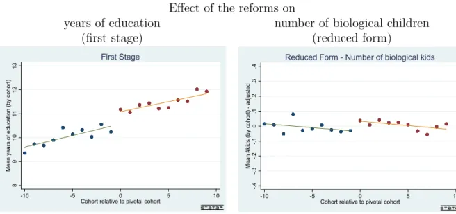
We first look at the effect of the reforms on years of education (first stage)

and the outcomes (reduced form parameters). The first stage and the effect

of the reforms on the number of biological kids are shown graphically in

Figure 1. In these graphs cohorts from different countries are normalized

with the compulsory schooling reforms, showing cohorts before and after the

event, respectively. The graph in the left panel shows the first stage: the

Effect of the reforms on

years of education number of biological children

(first stage) (reduced form)

8910111213Mean years of education (by cohort)

-10 -5 0 5 10

Cohort relative to pivotal cohort

First Stage

-.4-.3-.2-.10.1.2.3.4Mean #kids (by cohort) - adjusted

-10 -5 0 5 10

Cohort relative to pivotal cohort

Reduced Form - Number of biological kids

Figure 1. Effect of the reforms on years of education and on the number of biological children

reforms had an impact on years of education: mean years of schooling are higher for cohorts after the reforms. The reduced form graph (right panel) shows the (adjusted) number of biological kids for cohorts before and after the reforms.

The graph shows generally a decrease in fertility, but indicates a small positive jump at the pivotal cohort.

Table 3 shows the estimated coefficients of education on the number of biological kids and childlessness for three samples as well as for two differ- ent specifications of the country-specific trends in cohorts, a linear and a quadratic trend. Sample 10 includes at maximum 10 cohorts before and 10 cohorts after the reform, sample 7 is restricted to 7 and sample 5 to 5 cohorts before and after.

Consistently across samples and specification,

9The adjusted number of biological kids is the residual from a regression of the number of biological kids on a set of control variables (foreign born, proxy interview, interview year, cohort, country and country-specific linear trends in cohorts).

10In some countries 10/7/5 cohorts before and after are not available because the re- form was too early or too late for our sampling period or another reform was implemented.

the coefficients of the OLS regressions show the same signs as comparable correlation studies: years of education are negatively correlated with the number of biological kids and positively correlated with childlessness.

Furthermore, Table 3 reports reduced form estimates and first stage results of our model. The first stage results show that the reforms actually had an effect on schooling, one more year of compulsory education increased school- ing by about 0.2 – 0.3 years. The magnitudes of these coefficients are similar to other studies using compulsory schooling reforms in Europe (Brunello, Fabbri and Fort, 2009; Brunello, Fort and Weber, 2009). The F-statistics of the excluded instrument in the first stage ranges from about 18 to 25 in the specification with the linear country-specific trend, indicating that the instrument is sufficiently correlated with the endogenous variable. The specifications with the quadratic trends - where more variation in school attainment is filtered out - show smaller F-statistics, especially with sample 5. The reduced form estimates confirm the graphical inspection: one year of additional compulsory schooling increases the average number of children by between 0.06 and 0.08 depending on the specification and causes a large reduction in childlessness (by between 1 and 4 percentage points depend- ing on the specification); i.e. nearly up to 30 percent of the childlessness observed in our sample.

Two-stage least-squares estimates have the same signs as the reduced form

leading to an unexpected and interesting result: when we instrument years

of education with the number of compulsory schooling years, all coefficients

change their signs, i.e. schooling increases fertility. One additional year of

schooling raises the number of biological kids a women has by 0.2 – 0.3 and

decreases childlessness by about 7.5 – 13 percentage-points.

Table 3—Baseline results

Sample 10 Sample 7 Sample 5

l-trend q-trend l-trend q-trend l-trend q-trend A: # biological kids

OLS -0.033 -0.033 -0.033 -0.033 -0.031 -0.032

(0.005)*** (0.005)*** (0.005)*** (0.005)*** (0.006)*** (0.006)***

2SLS 0.205 0.284 0.312 0.294 0.188 0.311

(0.075)*** (0.095)*** (0.111)*** (0.134)** (0.064)*** (0.058)***

Reduced Form 0.064 0.078 0.083 0.068 0.064 0.056

(0.018)*** (0.019)*** (0.021)*** (0.021)*** (0.021)*** (0.024)**

B: Childlessness

OLS 0.007 0.007 0.007 0.007 0.006 0.006

(0.002)*** (0.002)*** (0.002)*** (0.002)*** (0.002)*** (0.002)***

2SLS -0.075 -0.127 -0.137 -0.121 -0.090 -0.137

(0.025)*** (0.039)*** (0.039)*** (0.051)** (0.025)*** (0.024)***

Reduced Form -0.023 -0.035 -0.036 -0.028 -0.031 -0.012

(0.006)*** (0.007)*** (0.007)*** (0.009)*** (0.008)*** (0.010)

First Stage 0.312 0.274 0.265 0.230 0.341 0.180

(0.065)*** (0.070)*** (0.063)*** (0.087)*** (0.068)*** (0.111)

F-Statistics 23.34 15.20 17.92 6.93 24.95 2.63

Observations 6,728 6,728 5,118 5,118 3,923 3,923

Note: Each coefficient represents a separate linear regression. Country-fixed effects, cohort-fixed effects, country-specific trends in birth cohorts (linear and quadratic), indi- cators for interview year, foreign born and proxy interview are included in all regressions.

Heteroscedasticity and cluster-robust standard errors in parentheses (clusters are country- cohorts). ***, ** and * indicate statistical significance at the 1-percent, 5-percent and 10-percent level.

As shown in Table 3, the main results are very robust across the different specifications - with respect to sampling and trend specifications.

B. Interpretation and Mechanisms

We observe a positive causal relationship between education and fertility.

On average, one year of education increases the number of biological kids by

about 0.27 and reduces childlessness by about 11 percentage-points. These

coefficients are large in magnitude and amount to about 14 percent and

85 percent of the dependent variable. We interpret these results as Local

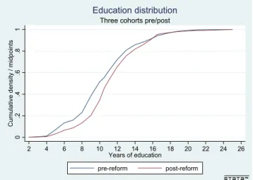
Average Treatment Effects, i.e. the effect of education on fertility for those who changed their schooling attainment because they were affected by the reforms (compliers). Since we are analyzing compulsory schooling reforms, our estimates might apply for those at the bottom of the education distri- bution. Figure 2 shows the distribution of years of education for our full sample three cohorts before and three cohort after the respective reforms.

The graph shows that the reforms had the largest effects for those with few years of education.

0.2.4.6.81Cumulative density / midpoints

2 4 6 8 10 12 14 16 18 20 22 24 26

Years of education

pre-reform post-reform Three cohorts pre/post

Education distribution

Figure 2. Education distribution before and after

Though it is not possible to identify compliers using observed data, since they are defined by means of counterfactual outcomes, we can characterize the population of compliers with respect to some interesting pre-treatment variables, as first suggested by Angrist (2004). The compliers population can be easily characterized by exploiting Bayes theorem (see Angrist (2004) for the details) when both the treatment (education) and the instrument

11Brunello, Fort and Weber (2009) show that this is true using quantile regressions.

(compulsory schooling) are binary variables. The extension of the result to continuous or discrete variables is not trivial, thus, we re-coded our treat- ment and instrument as binary.

Both surveys, SHARE and ELSA, include retrospective information about the respondent’s histories. We select pre- treatment variables that are similarly reported in the two surveys and can be considered as proxies for family attitudes and/or parental background, namely: (i) a binary indicator of whether the individual had few books (between 0 and 10) at home when aged 10; (ii) a binary indicator taking the value 1 if the individual has more (alive) siblings with respect to the country median (nearly 2 in almost all countries), 0 otherwise and (iii) a binary indicator taking the value 1 if the individual used to live in a large household, i.e. an household with more persons with respect to the country median in the sample, when aged 10.

We find that, with respect to the sample average, compliers tend to be: (i) 60 percent more likely to have had few books at home when aged 10; (ii) 97 percent more likely to have an above median number of siblings alive and iii) 86 percent more likely to come from large (i.e. above median) households.

We interpret these results as suggestive evidence that compliers tend to have a poorer background and be more family oriented with respect to the average individual in the sample.

If the causal effect of education on fertility is positive, why are those variables negatively correlated in OLS regressions? One explanation is, that

12The treatment is a binary indicator taking the value 1 if the individual’s actual years of education are equal or exceed the post-reform number of mandatory schooling years and 0 otherwise. The instrument is a binary indicator taking the value 1 for post-reform cohorts and 0 otherwise. For this exercise, we consider only countries for which the new mandatory schooling prescribed a one-year increase, so that the instrument coefficient has the same interpretation in all countries. The first stage on this sub-sample is smaller compared to our baseline results, but still statistically significant at 10 percent level.

the OLS results are biased downwards because of an omitted variables bias.

Assume the true econometric model to be

(3) Fertility

=

+

Edu

+

Family

+ . . . +

with Family capturing positive general attitudes towards the family or pref- erences for having children (γ

0 and

0). This variable will be positively related to fertility, but might be negatively related to years of education (COV (Edu, Family )

0) because women often have to decide between being family or career-oriented. If this variable is omitted from the regression and sufficiently correlated with education, the OLS coefficient on education will be biased downwards.

As described above, one possible channel why education may influence fertility is marriage behavior. We investigate whether education is related to the probability and the stability of marriage.

The upper panel of Table 4 shows the OLS and the 2SLS coefficients on marriage behavior. The OLS model exhibits that education is negatively correlated with an indicator variable of ever being married and positively related to being separated or divorced. When taking care of the endo- geneity of education again using compulsory schooling laws, all coefficients change their signs. One additional year of education increases the likelihood that a women got married by 6 percentage-points on average (6.3 percent).

The 2SLS estimates on separation/divorce are less precisely estimated in

13Normalize family orientation between 0 (no family orientation) and 1 (highest family orientation). If γ₂ = 1, then women with the highest level family-orientation have one child more than those with the lowest level family-orientation. In that case, a slope coefficient of 0.247 from the regression of family orientation on years of schooling (in the sample 10 model with linear trend) would explain the difference between the OLS and the IV model.

Table 4—Mechanisms

Sample 10 Sample 7 Sample 5

l-trend q-trend l-trend q-trend l-trend q-trend A: Marriage outcomes

Ever married

OLS -0.005 -0.004 -0.005 -0.005 -0.004 -0.004

(0.001)*** (0.001)*** (0.001)*** (0.001)*** (0.001)*** (0.001)***

2SLS 0.037 0.062 0.054 0.082 0.057 0.086

(0.017)** (0.026)** (0.022)** (0.041)** (0.020)*** (0.018)***

Separated/divorced

OLS 0.003 0.003 0.002 0.002 0.002 0.002

(0.001)** (0.001)* (0.002) (0.002) (0.002) (0.002)

2SLS -0.053 -0.056 -0.057 -0.077 -0.030 -0.041

(0.028)* (0.027)** (0.030)* (0.055) (0.022) (0.016)**

Observations 6,718 6,718 5,108 5,108 3,916 3,916

B: Quality of partner Years of education of partner

OLS 0.612 0.613 0.611 0.610 0.605 0.603

(0.020)*** (0.020)*** (0.022)*** (0.022)*** (0.025)*** (0.025)***

2SLS 0.532 0.821 0.613 0.629 0.648 0.594

(0.257)** (0.330)** (0.370)* (0.360)* (0.260)** (0.432)

Observations 3,705 3,705 2,784 2,784 2,123 2,123

C: Fertility men

# biological kids

OLS 0.002 0.002 0.001 0.000 0.001 0.000

(0.005) (0.005) (0.006) (0.006) (0.006) (0.006)

2SLS 0.013 0.102 0.076 0.235 0.172 -0.015

(0.076) (0.095) (0.087) (0.163) (0.091)* (0.057) Childlessness

OLS -0.004 -0.004 -0.004 -0.004 -0.004 -0.004

(0.001)** (0.001)** (0.002)*** (0.002)** (0.002)** (0.002)**

2SLS -0.017 -0.050 -0.041 -0.061 -0.055 -0.018

(0.020) (0.024)** (0.023)* (0.034)* (0.018)*** (0.016)

First Stage 0.446 0.471 0.468 0.425 0.484 0.275

(0.090)*** (0.102)*** (0.098)*** (0.132)*** (0.108)*** (0.118)**

F-Statistics 24.57 21.48 22.60 10.35 20.09 5.453

Observations 5,755 5,755 4,401 4,401 3,424 3,424

Note: Each coefficient represents a separate linear regression. Country-fixed effects, cohort-fixed effects, country-specific trends in birth cohorts (linear and quadratic), indi- cators for interview year, foreign born and proxy interview are included in all regressions.

Heteroscedasticity and cluster-robust standard errors in parentheses (clusters are country- cohorts). ***, ** and * indicate statistical significance at the 1-percent, 5-percent and 10-percent level.

the smaller samples but show similar magnitudes. One year of education decreases the likelihood of separation/divorce by 5 percentage-points (50 percent). Both results are in line with our results on fertility, i.e. education improves marriage outcomes, which in turn may increase fertility.

Next to its effect on the likelihood of marriage, education might improve the quality of the husband. The middle panel in Table 4 presents an analysis of this channel, based on a restricted sample of females with cohabiting partners. The OLS and 2SLS coefficients of the impact of female education on the years of education of their partners are very similar and amount to about 0.6, indicating a high degree of assortative mating. With respect to fertility, the education of the partner should increase household income and fertility. Note that these conditional effects on the quality of the partner for those who do have a partner are lower bounds to the unconditional effects of increased education on the probability for all women to have a highly- educated partner, because also the probabilities to get and stay married are higher for those women with higher education. The effects of education on marital outcomes and the quality of a potential partner are very consistent across the board: more education means a higher probability to live with a partner; a partner with higher education, as well.

While a higher probability to live with a partner will increase fertility,

what is the effect of mating partners with higher education? The lower

panel in Table 4 shows a fertility analysis for men in our sample. Our IV

estimates for males are typically smaller and less precise as those for females,

but are qualitatively similar: we find a positive causal effect of education on

the number of children and a negative one on the probability to be childless

as a man.

IV. Sensitivity analysis

This section presents several sensitivity checks and falsification tests. We will show that our estimates are not confounded with any selection biases.

In IV.A, we deal with the potential confounder of selective mortality. Fur- thermore, section IV.B present the robustness of our estimates to placebo reforms. We relax the assumptions on the functional form of the relationship between education and fertility by applying Count-data and Tobit models in IV.C and finally, we investigate the robustness of our estimates with respect to the selected reforms, countries and samples (IV.D).

A. Fertility and mortality

One potential confounder may be selective mortality. The older cohorts in our sample may be positively selected with respect to their health, since these individuals are still alive and able to participate in the SHARE and ELSA interviews. One concern is that these individuals might be selected with respect to fertility as well. If mortality is related to fertility in the way that childless women and women with fewer biological kids live longer, our estimates might reflect these patterns. This would mean that in our

14As discussed above, the standard model of labor supply predicts that a higher wage due to more education might increase or decrease fertility, depending on the magnitudes of the substitution and income effects. For those individuals in our sample, born in the first half of the 20th century, one may argue that this is true only for females. Males may have no substitution effect because they did not interrupt their working careers. According to this argumentation, one would expect the 2SLS coefficient to be larger for males than for females. However, several arguments can be made against this back-of-the-envelope comparison: income effects are not necessarily equal across gender, the fertility decision as well as other household-consumption decisions may not be made by the individual but at the couples-level and, an econometric argument, fertility of males might be measured with more error than the fertility of females.

“control” group (older cohorts with fewer years of compulsory education) the less fertile women might be over-represented.

One big advantage of our estimation strategy is that we are able to control for cohort-fixed effects. A large part of a potential mortality-related selec- tivity should thus already be eliminated. However, to eliminate any further biases, we pursue three different strategies: (i) we review the literature on the relationship between fertility and mortality, (ii) we restrict our analy- sis to younger cohorts and (iii) we estimate our models by controlling for differences in the life-expectancy of individuals born in different years and countries.

The literature on the relation between the number of children a wife has born and mortality is unclear; there are some papers showing correlation but no causal studies. Studies for previous centuries find a positive correlation between parity and mortality (Doblhammer and Oeppen (2003) looking at English peers starting from 1500 onwards as well as Smith, Mineau and Bean (2002) using Utah couples from 1860-1899). This might be due to medical risks directly related to childbirth. Studies using more recent data are in- conclusive: while Karsten Hank (2010) finds no effect for Germany, Lisa S.

Hurt, Carine Ronsmans and Suzanne L. Thomas (2006) in a meta-study find generally no relation between parity and mortality, if ever mortality risk is highest for women without children and those with more than four children.

In Table 5 we present several regressions that take care of a potential selective mortality bias. The first column replicates the baseline 2SLS re- sults for Sample 10 (with the linear country-specific trend in cohorts). The

15See also Doblhammer (2000) and Grundy and Tomassini (2005).

Table 5—Selective mortality

Baseline Recent Life-expectancy (see Table 3) cohorts control weight

# biological kids 0.205 0.236 0.202 0.254

(0.075)*** (0.089)*** (0.075)*** (0.094)***

Childlessness -0.075 -0.095 -0.073 -0.098

(0.025)*** (0.031)*** (0.025)*** (0.033)***

Observations 6,728 3,518 6,728 6,728

Note: Each coefficient represents a separate 2SLS linear regression based on Sample 10.

Recent cohorts are those born 1940–56, the Czech-Republic, England and the Netherlands are dropped from this regression. Country-fixed effects, cohort-fixed effects, country- specific linear trends in birth cohorts, indicators for interview year, foreign born and proxy interview are included in all regressions. Heteroscedasticity and cluster-robust standard errors in parentheses (clusters are country-cohorts). ***, ** and * indicate statistical significance at the 1-percent, 5-percent and 10-percent level.

coefficients in column 2 are based on a restricted sample of younger co- horts, those born 1940-1956. For this sample we had to exclude countries with early reforms (the Czech-Republic, England and the Netherlands). We argue that these cohorts are younger and selectivity on the basis of mor- tality differences is less severe. If our baseline results of a positive effect of education on fertility were driven by a selectivity bias, the estimates for recent cohorts should be significantly smaller than the baseline results. The estimated coefficients show that this is not the case; on the contrary: the numerical coefficients are somewhat higher.

For a further test, we collected data on life-expectancy at birth from the Human Mortality & Human Life-Table Databases.

While younger cohorts in our sample are generally aged below their life-expectancy, the older co- horts are above. In column 3, we added this variable to our regression. The

16The databases are provided by the Max Planck Institute for Demographic Research (www.demogr.mpg.de). The information is missing for some cohorts in Austria and Germany. We linearly predicted the life-expectancy for these cohorts. We use period- measures of life-expectancy at birth since cohort measures of life-expectancy at birth are currently not available for the cohorts we consider.

coefficients do not change. Column 4 presents 2SLS estimates of a weighted regression, with weight = 1/(age

age

life-expectancy , 1 otherwise, i.e. individuals that are aged above their life-expectancy get less weight in the regression. The 2SLS coefficients are, again, very similar to the baseline results.

All results presented in Table 5 are not sensitive to the specification (linear or quadratic trend) and the sampling window. Overall, the analysis suggests that the results are not driven by selective mortality of the respondents.

As described above, we only observe the children of the respondents if they

are still alive at the time of the interview. The older cohorts in our sample

might have had more children who are not alive anymore and therefore

not counted in the dependent variable. Thus, we have a measurement error

problem, with the measurement error being very likely to be correlated with

explanatory variables, the cohorts and most importantly our instrument,

years of compulsory schooling. This problem is very similar to the selective

mortality of the respondents themselves and the same sensitivity analysis

apply. If our results would stem from selective mortality of the children of

the respondents, the magnitude of the coefficients would get smaller if only

recent cohorts are used for the analysis (for whom the measurement error

should be smaller) or if life-expectancy is accounted for. As Table 5 shows,

this is not the case. Furthermore, the average age at first birth of women in

our sample is nearly 25 and their age at the time of the interview is 65 on

average. Thus, their oldest child should be aged only 40 at the time of the

interviews.

B. Placebo treatments

As compulsory schooling reforms affect cohorts differently we might be concerned that our school reform variables pick up some unspecified time trend in the countries. To test for this, we are using a placebo reform exercise. Similar to Black, Devereux and Salvanes (2008), we introduce a placebo treatment where we add a hypothetical compulsory schooling reform for each of our countries, either three or five years in the future.

This placebo reform should not have any impact on fertility. If we find an impact, our results might be driven by other unobserved mechanisms (like selective mortality or time trends). As the placebo reform should have no impact on attended years of schooling, we can only use the reduced form estimates to test for a placebo effect.

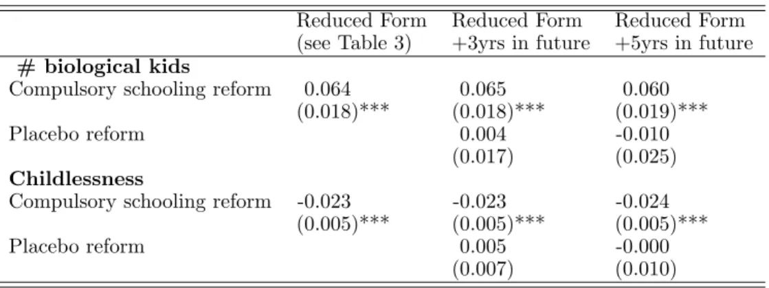
Table 6 shows the reduced form estimates for the number of biological kids and childlessness (again for sample 10 with linear time trends). In both panels, the reduced form of the baseline model is given in column 1. In columns 2 and 3, the results of the placebo tests are given. Adding placebo schooling reforms three years in future (column 2) and five years in future (column 3) does not alter the reduced form estimates of the original reforms.

Furthermore, none of the future laws has any impact on fertility. The same results are obtained with sample 7 and with the quadratic specification of the time trends.

17Note that we have to include the real compulsory schooling reforms in the regressions as well, as for some cohorts placebo and real reform overlap.

Table 6—Placebo treatments

Reduced Form Reduced Form Reduced Form (see Table 3) +3yrs in future +5yrs in future

# biological kids

Compulsory schooling reform 0.064 0.065 0.060

(0.018)*** (0.018)*** (0.019)***

Placebo reform 0.004 -0.010

(0.017) (0.025)

Childlessness

Compulsory schooling reform -0.023 -0.023 -0.024 (0.005)*** (0.005)*** (0.005)***

Placebo reform 0.005 -0.000

(0.007) (0.010)

Note: Each column and panel represents a separate regression based on Sample 10.

Country-fixed effects, cohort-fixed effects, country-specific linear trends in birth cohorts, indicators for interview year, foreign born and proxy interview are included in all regres- sions. Heteroscedasticity and cluster-robust standard errors in parentheses (clusters are country-cohorts). The number of observations in all specifications is 6,728. ***, ** and

* indicate statistical significance at the 1-percent, 5-percent and 10-percent level.

C. Functional form

In previous sections, we presented results based on the estimation of lin- ear regression models. However our data present two characteristics that may be relevant for the choice of the regression model: first, the number of children in a family takes only non-negative integer values, so that count data regression models would be more appropriate choices; second, our data on the number of biological children are (right) censored at four, thus we should consider regression models that allow for censoring. This section is devoted to present evidence on the robustness of our results to differ- ent modeling choices. We consider in turn: (i) Poisson regression models (estimated by maximum likelihood); Poisson regression models that allow for right censoring (Raciboski (2011)); tobit regression models and discuss results in turn.

Table 7 reports results of Poisson regression models estimated by maxi-

Table 7—Poisson regression models results

No censoring Right censoring (4)

(1) (2) (3) (4) (5) (6)

edu edu^a resid^a edu edu^a resid^a

Coefficient -0.018^∗∗∗ 0.125^∗∗ -0.142^∗∗ -0.020^∗∗∗ 0.132^∗∗ -0.152^∗∗

[-0.02,-0.01] [0.02,0.35] [-0.37,-0.04] [-0.03,-0.01] [0.01,0.39] [-0.41,-0.03]

APE^b -0.034^∗∗∗ 0.182 -0.208^∗ -0.033^∗∗∗ 0.171 -0.197^∗

[-0.04,-0.02] [0.00,0.56] [-0.59,0.00] [-0.04,-0.02] [0.00,0.52] [-0.55,0.00]

Note: 95 percent confidence intervals (CI) are in brackets. Each column and panel represents a separate regression based on Sample 10. Country-fixed effects, cohort-fixed effects, country-specific linear trends in birth cohorts, indicators for interview year, foreign born and proxy interview are included in all regressions.***, ** and * indicate statistical significance at the 1-percent, 5-percent and 10-percent level.

a Average estimates over 500 bootstrap replications.

b APE stands for Average Partial Effect on the average number of children at mean values of covariates in the sample. Columns (1) and (4): education treated as exogenous.

Columns (2) and (5): education treated as endogenous. CI in columns (1) and (4) are based on standard errors estimated by Delta-method and normal approximation. CI in columns (2), (3) and (5), (6) are based on the estimator’s empirical c.d.f. .

mum likelihood. The left panel presents the coefficient estimates and average partial effects on the average number of children for a simple Poisson regres- sion model, while the right panel presents estimates of a model that allows for right-censoring at four. In Columns (1) and (4) education is treated as exogenous: the average partial effects can be compared with OLS marginal effects in the first column of Table 3. In columns (2) and (5) education is endogenous (compare with the 2SLS results in the first column of Table 3).

In Poisson regression models, instrumental variable estimation is based on a control function approach. In practice, we proceed in two steps. In the first step, we generate the residuals from the first stage regression, i.e. the regres- sion of years of education on years of compulsory schooling. In the second step, the generated residual is added as a regressor in the outcome equation.

This allows to isolate - in the outcome equation - the variation in education

that is exogenous, i.e. driven only by compulsory schooling reforms. Table 7 reports also the coefficient of the generated regressor: rejecting the null hypothesis that the coefficient of the residual is zero can be interpreted as evidence of endogeneity. Since the outcome equation in the second step in- cludes generated regressors, we use bootstrap with 500 replications and base our confidence intervals on the resulting empirical cumulative distribution function of the estimator.

As in previous sections, when we do not take endogeneity of education into account we find a negative relationship between years of schooling and the number of children, with the magnitude of this correlation being essentially the same s the one delivered by OLS regressions. When we isolate the exogenous variation in years of education driven by compulsory schooling laws, the sign of the relationship is reversed: the average partial effect on the average number of children is around 0.18, very similar to our 2SLS estimates albeit less precise (Columns (1) and (2)). The same holds when we allow for censoring (see columns (4) and (5) in Table 7). In addition, the null hypothesis that the residual coefficient is zero is always rejected, pointing to endogenity of education in the fertility equation.

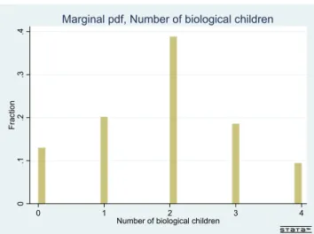
Since the distribution of the number of births is approximately normal (see Figure A1 in the Appendix), we also estimate Tobit regression models by maximum likelihood (Table 8). By estimating a Tobit model, we model jointly the decision on whether to enter motherhood and the decision on the actual number of children, allowing for correlation between these choices.

18This comes at the expense of imposing the same coefficient on education in the equation determining the two choices, as in standard Tobit models. Consider that it is difficult to think about an instrument for education for the motherhood equation than can be excluded from the equation for the number of children, once the woman enters motherhood.

Table 8—Tobit regression models results

Right censoring (4) Right censoring (4)

& Corner solution (0)

(1) (2) (3) (4)

Coefficient -0.037 0.217 -0.043 0.274

(0.005)^∗∗∗ (0.082)^∗∗∗ (0.006)^∗∗∗ (0.098)^∗∗∗

Average Partial Effects APE^a on

P rob[Y = 0] 0.003 -0.026 0.005 -0.036

(0.001)^∗∗∗ (0.011)^∗∗∗ (0.001)^∗∗∗ (0.013)^∗∗∗

E[Y|Y >0] -0.029 0.157 -0.031 0.180

(0.004)^∗∗∗ (0.058)^∗∗∗ (0.004)^∗∗∗ (0.063)^∗∗∗

E[Y|1< Y <4] -0.015 0.064 -0.014 0.062 (0.002)^∗∗∗ (0.023)^∗∗∗ (0.002)^∗∗∗ (0.021)^∗∗∗

Note: Each column and panel represents a separate regression based on Sample 10.

Country-fixed effects, cohort-fixed effects, country-specific linear trends in birth cohorts, indicators for interview year, foreign born and proxy interview are included in all regres- sions. Cluster adj. standard errors are in parentheses. ***, ** and * indicate statistical significance at the 1-percent, 5-percent and 10-percent level. Columns (1) and (3): edu- cation treated as exogenous. Columns (2) and (4): education treated as endogenous. ^a APE stands for Average Partial Effect at mean values of covariates in the sample.

We allow alternatively for right censoring (columns (1) and (2) in Table

8) and for right censoring and corner solutions at 0 (columns (3) and (4)

in Table 8). Using the estimates, we assess the average partial effect of

education on the probability to be childless and on the average number of

children for women who decide to: (i) have at least one child; (ii) have more

than 1 but not more than 4 children. Columns (1) and (3) refer to the

estimation results when education is treated as exogenous while in Columns

(2) and (4) education is treated as endogenous. We confirm previous results

in terms of direction of the effects: the association between education and

fertility is negative while the causal effect is positive, i.e. education increases

fertility and reduces childlessness. While the magnitude of the effect on the

average number of children, conditional on entering motherhood, is similar

to those estimated using linear regression models, the magnitude of the effect

on childlessness is smaller, around 50 percent lower than the one previously estimated, which might be due to the restriction imposing equal coefficients in the Tobit model.

Overall, our results are robust to the choice of the regression model in terms of direction of the effects on completed fertility and childlessness and also with respect to the magnitude of the effect on the average number of children. This may be due to the fact that the amount of censoring is very small (less than 5 percent of the sample), and that the distribution of the number of births is approximately normal.

D. Further robustness

Last but not least, we show that our results are robust to the selection of samples, the choices of reforms and the countries we are analyzing. As de- scribed above, our samples are not necessarily symmetric around the pivotal cohort, since in some countries 10, 7 or 5 cohorts before and after the reform are not always available. In some countries, the reform was too early or too late for our sampling period or another reform was implemented early on.

Table 9 shows the 2SLS estimates when we restrict our samples to symmetric windows around the reforms. The results are very robust to that.

In some countries, more than one compulsory schooling reforms were im- plemented in our observation period. Table 9 shows the 2SLS estimates when we use all those reforms for our analysis, again the results are very robust.

A further sensitivity check is based on the selection of countries we are

using. Table 10 presents ours results, when we drop one country at a time

from the sample. Again, the results are very robust.

Table 9—Sensitivity to samples and reforms

Symmetric windows All reforms

Sample 10 Sample 7 Sample 5 Sample 10 Sample 7 Sample 5

# biological kids 0.199 0.270 0.197 0.145 0.214 0.214

(0.096)** (0.118)** (0.077)** (0.063)** (0.097)** (0.097)**

Childlessness -0.118 -0.143 -0.102 -0.070 -0.127 -0.098

(0.038)*** (0.047)*** (0.031)*** (0.021)*** (0.033)*** (0.024)***

Observations 5,784 4,731 3,830 8,733 6,683 5,206

Note: Each coefficient represents a separate 2SLS regression. All reforms include addi- tional reforms in the Czech-Republic (1953/1960), France (1936) and the Netherlands (1947/1950). Country-fixed effects, cohort-fixed effects, country-specific linear trends in birth cohorts, indicators for interview year, foreign born and proxy interview are included in all regressions. Heteroscedasticity and cluster-robust standard errors in parentheses (clusters are country-cohorts). ***, ** and * indicate statistical significance at the 1- percent, 5-percent and 10-percent level.

Table 10—Sensitivity to countries

One reform per country All reforms

# biological kids Childlessness Obs # biological kids Childlessness Obs

w/o AUT 0.205 -0.073 6,303 0.141 -0.069 8,308

(0.079)*** (0.026)*** (0.067)** (0.022)***

w/o CZE 0.197 -0.077 6,337 0.146 -0.085 7,335

(0.074)*** (0.026)*** (0.074)** (0.027)***

w/o DNK 0.306 -0.092 5,760 0.202 -0.085 7,765

(0.112)*** (0.035)*** (0.074)*** (0.027)***

w/o ENG 0.222 -0.089 4,329 0.173 -0.074 6,334

(0.083)*** (0.029)*** (0.060)*** (0.022)***

w/o FRA 0.206 -0.089 5,912 0.092 -0.071 7,531

(0.087)** (0.029)*** (0.070) (0.022)***

w/o GER 0.180 -0.067 6,378 0.121 -0.063 8,383

(0.069)*** (0.023)*** (0.061)** (0.020)***

w/o ITA 0.195 -0.069 5,619 0.105 -0.066 7,624

(0.153) (0.056) (0.097) (0.036)*

w/o NLD 0.224 -0.082 6,458 0.199 -0.066 7,851

(0.081)*** (0.027)*** (0.066)*** (0.022)***

Note: Each coefficient represents a separate 2SLS regression based on sample 10.

Country-fixed effects, cohort-fixed effects, country-specific linear trends in birth cohorts, indicators for interview year, foreign born and proxy interview are included in all regres- sions. Heteroscedasticity and cluster-robust standard errors in parentheses (clusters are country-cohorts). ***, ** and * indicate statistical significance at the 1-percent, 5-percent and 10-percent level.

V. Concluding remarks

We study the effects of education on fertility for women in 8 European countries using exogenous variation in education brought along by manda- tory schooling reforms in the 1930s-60s. Contrary to conventional wisdom, we show that more schooling leads, in fact, to higher fertility. Using our instrumental variables estimates, we find that one additional year of school- ing increases the number of children by 0.2 - 0.3, whereas the probability to remain childless falls by 7.5 - 13 percentage-points with somewhat smaller numbers in the Tobit specification. A number of falsification and robustness tests, like placebo reforms, tests for functional form or selective mortality in the sample strongly corroborates these findings.

What are the mechanisms behind these results? We argue that compulsory

schooling reforms target a specific group in the population: those at the

lower end of the educational distribution. For these women the income

effect of increased schooling may outweigh the substitution effect on the

labor market and higher education results in higher fertility rates. Our

evidence suggest that compliers to compulsory schooling reforms are more

likely to have been grown up in larger and also poorer families with respect

to the average woman in the sample. Growing up in a large family might

generate a positive attitude towards family and having kids. Next to the

labor market effects, the marriage market may also play a role in shaping

fertility. We present evidence that additional schooling leads to i) a higher

probability to get married, ii) a lower divorce/separation rate and iii) a

potential partner who is better educated and, thus, more inclined to have

(or approve of) children himself.

REFERENCES

Adsera, Alicia. 2005. “Vanishing children: From high unemployment to low fertility in developed countries.” American Economic Review Papers and Proceedings, 95: 189–193.

Ahn, Namkee, and Pedro Mira. 2002. “A note on the changing re- lationship between fertility and female employment rates in developed countries.” Journal of Population Economics, 15: 667–682.

Angrist, J. 2004. “Treatment Effect Heterogeneity in Theory and Prac- tice.” The Economic Journal, 114: C52–C83. Issue 494.

Angrist, Joshua, and Alan Krueger. 1991. “Does Compulsory School Attendance Affect Schooling and Earnings?” Quarterly Journal of Eco- nomics, 106: 979–1014.

Becker, Gary. 1965. “A theory of the allocation of time.” Economic Jour- nal, 75: 493–517.

Becker, Gary, and H. G. Lewis. 1973. “On the interaction between quantity and quality of children.” Journal of Political Economy, 81: S279–

S288.

Behrman, Jere R., and Mark R. Rosenzweig. 2002. “Does Increasing Women’s Schooling Raise the Schooling of the Next Generation?” Amer- ican Economic Review, 92/1: 323–334.

Black, Sandra E., Paul J. Devereux, and Kjell G. Salvanes. 2008.

“Staying in the classroom and out of the maternity ward? The ef-

fect of compulsory schooling laws on teenage births.” Economic Journal,

118(July): 1025–1054.