The Evolution of Climate Over the Last Millennium

(1)

The Evolution of Climate Over the Last Millennium

P. D. Jones,* T. J. Osborn, K. R. Briffa Knowledge of past climate variability is crucial for understanding and modeling current and future climate trends. This article reviews present knowledge of changes in temperatures and two major circulation features—El Nin˜o–Southern Oscillation (ENSO) and the North Atlantic Os- cillation (NAO)—over much of the last 1000 years, mainly on the basis of high-resolution paleoclimate records. Average temperatures during the last three decades were likely the warmest of the last millennium, about 0.2°C warmer than during warm periods in the 11th and 12th centuries.

The 20th century experienced the strongest warming trend of the millennium (about 0.6°C per century). Some recent changes in ENSO may have been unique since 1800, whereas the recent trend to more positive NAO values may have occurred several times since 1500. Uncertainties will only be reduced through more extensive spatial sampling of diverse proxy climatic records.

The instrumental record is generally considered not to be long enough to give a complete picture of climatic variability. Recent records are also likely already influenced by human actions (1). It is crucial, therefore, to extend the record of climatic variability beyond the era of instrumental measurements if we are to understand how large natural climatic variations can be, how rapidly climate may change, which internal mechanisms drive climatic changes on regional and global scales, and what external or internal forcing factors control them (2). At present, paleoclimatology is very far from achieving season-specific histories for different climate variables at the regional scale; which is the detailed picture we need in our search for an unambigu- ous “fingerprint” of the climate response to increasing greenhouse gas emissions (1, 2).

Interest has, therefore, focused initially on large-scale climate features, particularly mean hemispheric temperatures and the behavior of major climate phenomena like the El Nin˜o–Southern Oscillation (ENSO) and the North Atlantic Oscillation (NAO) (3).

Here we review the current knowledge of large-scale climate variability during the last 1000 years, highlight some problematic is- sues, and point to where additional research is needed.

Northern Hemisphere Temperature Relatively widespread (4) instrumental data exist for the land and marine regions of the Northern Hemisphere (NH) back to the mid- 1850s (5). These data show that since 1861, annual average temperatures have warmed by

0.6°C, but with a marked seasonal contrast:

winters have warmed by nearly 0.8°C and summers by only 0.4°C. The warming has occurred in two pronounced phases, from about 1920 to 1945 and from 1975 to the present (5).

Several attempts (6–10) have been made recently to extend this record of temperature variations across the NH to cover the last 1000 years. All are based on the rationale that large-scale temperature variability can be represented sufficiently well by integrating data from a limited number of geographically scattered indicators or “proxies” (11) of variability of past climate. Proxies are of two basic kinds, natural ( physical or biological) and documentary (written) archives. Figure 1 illustrates typical ranges of high-resolution temperature-sensitive proxies that have been used by (6–10) and regions where there is the potential to obtain additional proxies. Easily the most numerous of the proxy data used by (6–10) are derived from trees (ring density, ring width, and wood isotopes), followed by ice cores (isotope ratios, accumulation rates, and melt layers) and corals (isotopes, cation ratios, and growth thicknesses). Only one documentary series has been included because many are discontinuous and use mate- rial that is anecdotal in nature (12). Even this one series contains meteorological records for the 19th and 20th centuries (13), making it difficult to quantify its reliability during earlier centuries.

All of the curves in Fig. 2, with the ex- ception of that based solely on tree-ring density data (8), make use of some instrumental data (14) from the mid-17th century onwards.

There is no ambiguity in the interpretation of directly recorded temperature and precipitation observations, and they can be readily averaged to represent precise seasons. In con-

trast, natural and documentary proxies fre- quently represent the combined influences of climatic and nonclimatic factors, and their climate-related variability may reflect both temperature and precipitation to varying ex- tents. Furthermore, different proxies (and even the same proxy type sampled at different locations) may record climate at different times of the year.

The common approach to climate reconstruction from proxies is to use statistical regression to establish a connection between climatic observations and the variability of the proxy over some period of overlap (15).

This provides a transfer function that enables the proxies to be used as predictors of past climate but makes large assumptions about the temporal and spatial stability of the climate “signal” represented in these proxy records.

In Fig. 2A, two of the curves [(7) in orange and (9) in blue] are equally weighted averages of a small number of proxies [13 and 10, respectively], both subsequently re- gressed against a single “target” NH temperature series (16). This procedure assumes that the same NH mean signal is contained within the variance of each individual proxy and that simply averaging all of them together cancels the variability that represents random noise and local-scale variability. Studies based on modern instrumental records suggest that mean hemispheric trends can be reliably re- produced from only a few regional series (17–19), provided they are drawn from areas with wide spatial coherence and assuming that the co-variance structure of temperature variability during the calibration period re- mains the same for earlier periods.

The other two curves in Fig. 2A [(6,10) in red and (8) in green] employ many more series as predictors and use more complex multivariate regression. This assumes that some proxies are consistently more representative of the NH signal than others and that greater emphasis can be placed on them. The weighting is determined by the strength of their association with direct climate observations over a calibration period, and differences of sign or seasonality in the response of different variables to the same climate can be accommodated. Mann et al. (6, 10) used many different types of proxy records with a wide range of direct climate responses (to both temperature and precipitation over different seasons) to estimate annual temperature across a large fraction of the NH. Al- Climatic Research Unit, University of East Anglia,

Norwich NR4 7TJ, UK.

*To whom correspondence should be addressed. E- mail: p.jones@uea.ac.uk

R E V I E W

(2)

though the method of Briffaet al.(8) allowed nonuniform weighting of proxies, in practice the weighting depended only slightly on the association with direct climate observations because they selected similarly summer-re- sponsive tree-ring density series as regional predictors before estimating a large-scale NH temperature average.

The best quality data are available for the most recent past (⬃1880 –1980). This applies not only to the amount and coverage of instrumental observations, but also to the quality and number of proxy records. Because more data exist and the fit between climate observations and proxies can be optimized over relatively recent times, earlier estimates of NH temperatures are almost bound to be less representative of reality than is apparent from the modern regression. It is, therefore, vitally important to take account of uncertainties in proxy-based climate reconstructions, even in recent periods, and to be mindful of the extent to which they have been realisti- cally calculated for earlier times (20).

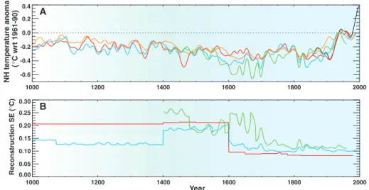
Bearing in mind the 1 standard error confidence levels for three of the NH reconstructions (Fig. 2B), how have NH mean temperatures varied over the last millennium? For the last 300 years, the reconstruction uncertainties are quite similar, amounting to about 0.1°C on a 30-year time scale. Data are relatively abundant over this period, and the records all indicate rapid warming in the 20th century, with temperatures about 0.2°C above the millennial mean throughout the middle and later part of the century. NH temperatures underwent an abrupt cooling in the early decades of the 19th century, following a period near their long-term mean during the 18th century. The whole of the 17th century was cool. This is accentuated in the summer records, most markedly over the northern land areas (8), where the mean 17th-century

temperature was about 0.5°C lower than between 1961 and 1990. The confidence levels for this reconstruction (8) are wider over this period (⬃0.2°C), but still allow us to con- clude that this was probably the longest period of sustained cold conditions during the millennium. In the annual records, this cool period is longer but less extreme than that experienced in the early 19th century (6, 7, 10).

Before 1600, there are no instrumental records and far fewer proxy series, resulting in much higher uncertainty in the reconstructions (between about 0.1° and 0.25°C). Nev- ertheless, the individual records present a consistent story of generally increasing temperature back to 1000, with the first century of the millennium on average near 0.1°C above the millennial mean, but still 0.1°C below the 1961 to 1990 average. Only three of the multi-proxy reconstructions reach back to the start of the millennium, where they are based on very few individual proxy records.

Several of these records are used in all three studies, and some have additional uncertainty (20,21) not accounted for in the estimate of regression uncertainty (Fig. 2).

Thus, present evidence points to warm 11th and 12th centuries, but with a degree of uncertainty which allows speculation that the start of the millennium was as warm as most of the 20th century. This evidence still leaves considerable room for improvement. During the last 30 years, however, directly measured temperatures (black line in Fig. 2) have risen sharply, beyond even the upper range of uncertainty (2 standard errors above the reconstructed value) surrounding the warmest earlier reconstructions. On the basis of this evidence, there is little room to doubt (22) that the last few decades of the millennium have been significantly warmer than any others, when viewed across the NH as a whole.

Southern Hemisphere Temperature Instrumental coverage is markedly poorer in the Southern Hemisphere (SH) than in the NH, with regular surface measurements available, even now, from only two-thirds of the surface. SH temperature trends are similar to those in the NH, but show no seasonal contrast. Some differences in timing are apparent and may be important. The SH average shows greater recent warming than earlier in the 20th century, and there is no evidence of the slight 1945 to 1975 cooling seen over many NH land areas (5). Instrumental data from Antarctica are only available since the mid-1950s. They show a temperature rise until the early 1970s, with little change since then (23). There is, therefore, an even greater need for proxy data, although the lack of long instrumental records also makes calibration of proxies (not only in the Antarctic, but over most of the SH ocean) difficult.

The number of natural proxy records available for the SH is nearly two orders of magnitude smaller than for the NH, partly due to the smaller landmass, but also because far less research has been undertaken. The situation is improving, with many recent ad- vances in tree-ring, ice-core, and coral reconstructions (24). Documentary evidence is limited to sources in South America (Fig. 1) since 1500, although most published work relates to El Nin˜o variability (25). Recently, the reliability of this documentary reconstruction has been questioned (26).

Multi-proxy averages for the SH have been assembled by Joneset al.(9) and Mann et al.(27). The former study (9) is based on only seven equally weighted predictors, whereas the latter (27) attempts to reconstruct only those regions where instrumental temperature records are fairly complete from 1902 to 1980, limiting the study mostly to areas north of 45°S. Both (9,27) stress that it Fig. 1.Schematic map in- dicating the principal regions from which well- dated pre-1750 temperature information could potentially be obtained with approximately annual resolution. Addition- al proxies providing such information in more limited regions have not been included; neither have the many proxies providing precipitation or drought information, nor those providing temperature information with only decadal-to-century time scale resolution.

(3)

is dangerous to place too much reliance on these curves, because the associated errors are likely greater than those for the NH (28).

The two SH reconstructions (Fig. 3) show little trend in temperature since 1600, except for the quasi-linear rise during the 20th century. The Joneset al.(9) series shows greater variability, probably because it is an average of fewer series than Mannet al.(27). Few of the warm or cool decades and longer periods coincide with the same periods in the NH (29). Neither series, for example, shows the signature of cold 17th, milder 18th, and cooler 19th centuries that is evident in the NH (Fig. 2).

El Nin˜o–Southern Oscillation

In order to understand climate variability and attribute past climate variations to particular causative factors, it is necessary to reconstruct more than just hemispheric mean temperature over the past 1000 years. We need to know how external forcings of the climate system (such as solar insolation and explo- sive volcanic eruptions) have changed during the same time period (30–32), and we also need to reconstruct the behavior of phenomena that are internal to the climate system.

Here we consider two very important internal phenomena, each of which can influence hemispheric and global temperatures: the ENSO and the NAO.

Two difficulties arise when attempting to reconstruct the past behavior of these (and other) modes of climate variability. First, no climate proxy directly measures variability of the atmospheric circulation, but instead

records its local environmental influence (through the deposition of transported mate- rial or through the indirect effects on temperature or precipitation at the proxy sites). Sec- ond, the likelihood of changes in the climatic influence of a phenomenon is an issue over long periods of time, particularly for locations more distant from the key centers of dynamical or physical interaction that are responsible for generating the phenomenon.

Therefore, proxies for sea surface temperature (SST) in the equatorial Pacific, where the key processes responsible for ENSO take place, are more direct and less likely to be affected by changes in the climatic influence of ENSO than terrestrial proxies. Additional- ly, caution must be exercised when assessing the relation between the reconstructed variability of a particular phenomenon and reconstructed temperature or precipitation variations to avoid circularity if the same climate proxies are used to reconstruct both (33).

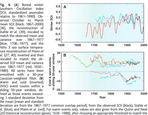
ENSO is the dominant coupled atmo- sphere-ocean mode of interannual climate variability, affecting most of the tropics and subtropics and many mid-latitude regions of North and South America and eastern Asia (34, 35). Instrumental measures of the phe- nomenon are either atmospheric [the South- ern Oscillation Index (SOI)] or oceanic [for example, SSTs in the Nin˜o 3 region (150 to 90°W, 5°N to 5°S)] and extend back to the mid-19th century (36–38). Acknowledging the difficulties outlined above, some reconstructions of ENSO variability before the instrumental record have been attempted (Fig.

4A) (39, 40). The Stahle et al. (39) recon-

struction is based on tree-ring parameters, principally from the southwestern United States and northern Mexico, whereas the Mannet al.(27,40) series is a reconstruction of the Nin˜o 3 SST series (37) using a multi- proxy database from tropical locations, including a similar set of tree-ring predictors to those used in (39). Both series show similar interannual and interdecadal variability back to the early 1700s (38). On the 30-year time scale (Fig. 4A), many of the low-frequency features agree (41), although the Mannet al.

(27, 40) series tends to have more warm phase (low SOI) events before 1800. The recent 25-year period during which warm phases have dominated appears to be unique in the tree-ring– based reconstruction and in the Mannet al.(27,40) series since 1800, but the uncertainty in the reconstructions needs to be fully quantified before this statement can be made with confidence.

Frequency statistics of warm (El Ninõ) and cold (La Ninã) events are as important as the low-frequency behavior of ENSO. Warm- phase occurrence shows little long-term change since 1750 in two of the series (around 7 to 11 events per 50 years), whereas (39) shows fewer (5 to 7) warm events before 1900 (Fig. 4B). The longer series indicate more frequent El Ninõ occurrences between 1700 and 1750 (27,40) and before 1630 (25).

La Ninã events show greater changes, with more frequent events during the 20th century compared with earlier centuries. Before 1850, both reconstructions indicate only 2 to 5 La Ninã events per 50 years. Whether this change is real is debatable: it may be that drought influences tree growth much more strongly during El Ninõ conditions than do heavy rains during La Ninã.

North Atlantic Oscillation

The second most important mode of (atmospheric) variability is the NAO. Studies of the

Fig. 2.(A) Northern Hemisphere surface temperature anomalies (°C) relative to the 1961–1990 mean (dotted line). Annual mean land and marine temperature from instrumental observations (black, 1856–1999) (5) and estimated by Mannet al.(red, 1000 to 1980) (6,10) and Crowley and Lowery (orange, 1000–1987) (7). April to September mean temperature from land north of 20°N estimated by Briffaet al.(green, 1402–1960) (8) and estimated by re-calibrating (blue, 1000 to 1991) the Joneset al.Northern Hemisphere summer temperature estimate (9,16). All series have been smoothed with a 30-year Gaussian-weighted filter. (B) Standard errors (SE, °C) of the temperature reconstructions as in (A), calculated for 30-year smoothed data. The proxy average series (6–10) do not extend to the present because many of the constituent series were sampled as long ago as the early 1980s.

Fig. 3.Southern Hemisphere surface temperature anomalies (°C) relative to the 1961–1990 mean (dotted line). Summer (December to Feb- ruary) land and marine temperature from instrumental observations (black, 1856–1999) (5) and from estimates by Joneset al.(blue, 1600–1991) (9). Annual mean (January to De- cember) land and marine temperature estimated by Mannet al. (red, 1700–1980) (27). All series have been smoothed with a 30-year Gaussian-weighted filter.

(4)

phenomenon (and its relative, the Arctic Os- cillation) have had a resurgence since the work of Hurrell (42, 43). Variations in the NAO generate much of the interannual variability in winter climate over Europe and are also implicated in more widespread warming over the past few decades (44). There is a pressing need, therefore, to extend our knowledge of NAO variability over longer periods to assess whether recent variations were unique. Instrumental records based on pressure data at the NAO’s two centers of action (Iceland and the Azores/Iberia) extend back to the 1820s (45). Several extended reconstructions from ice-core, tree-ring, and documentary parameters have been produced (46–49), but recent intercomparisons reveal little agreement between some of the indices before the 1820s (49, 50). As with the SOI, the NAO is defined on the basis of atmospheric pressure data, and the NAO’s influence on surface variables at specific locations may change, as has been observed during the instrumental period especially for the more indirect teleconnections (51).

Two new reconstructions show partially consistent co-variability (on interannual time scales) back to 1500 (Fig. 5) (52–54). The reconstructions cover the December to March winter period, when the NAO exerts its strongest influence on surface climate in eastern North America, the Atlantic, Europe, and North Africa (42– 44, 51). One of the reconstructions (53) is based on early European instrumental and documentary data (including some pressure series); the other (52) is based on tree-ring and ice-core data from regions on both sides of the North Atlantic.

Both use varying networks of proxies to reconstruct earlier periods (each calibrated over much of the post-1875 period). The quality of each reconstruction is reduced for the earliest periods when fewer proxies are available.

The effects of low-frequency changes in boundary conditions (such as consistently cooler SST values compared with the 20th- century average, which might be inferred from Fig. 2) are only incorporated to the extent that such variability is reflected in the proxies used.

The instrumental and documentary series agrees best with the observations, but this is expected because extensive pressure observations are included back to the mid-19th century. On 30-year time scales, agreement between the series is poorer than on the interannual time scale, particularly before 1780.

For the 18th century and earlier, explained variances are higher for the instrumental and documentary than for the natural proxy reconstruction. The instrumental and documentary series reconstructs mainly negative- phase NAO values before 1800, whereas the natural proxies imply more positive-phase NAO winters. Recent, strongly positive values of the NAO are probably not unique, as they also occurred during the early 20th century and in some earlier periods.

Concluding Remarks

Multi-proxy temperature reconstructions for the NH show that the recent 30-year period is likely to have been the warmest (about 0.2°C above the 1961 to 1990 average) of the millennium, with the warmest century (by about 0.1°C) likely to have been the 20th. The first half of the millennium was milder (0.2°C below the 1961 to 1990 average) than the 1500 to 1900 period. The coolest century was the 17th (– 0.4°C) followed by the 19th, sep- arated by a milder 18th century. The results provide some support for earlier work, which postulated two epochs during the millennium, the Little Ice Age [LIA, variously dated, but 1550 –1900 encompasses most published dates (55,56)] and the Medieval Warm Pe- riod [MWP, also variously dated, but 900 – 1200 encompasses most dates (57)]. The post-1400 results are similar to those produced by Bradley and Jones (55) in 1993. The SH temperature reconstructions are shorter and less reliable; they do indicate cooler conditions before 1900, but not the same inter- centennial variation evident in the north.

The last couple of decades have seen dra- matic improvements in paleoclimatology with at least two orders of magnitude more information (involving a wider range of proxies from more diverse locations), in compar- ison to around 1975. Much of the basic raw data is now available via the Internet (58), facilitating the assembly of multi-proxy data- bases. Together with improved statistical techniques, this expansion in available proxy data has led to more accurate reconstruction of the climate of the past millennium.

To improve our knowledge of climate history further, we need yet more proxy data:

many more earlier data to provide better global coverage and more recent data to en- able better interpretation. We need to fill in the large geographic gaps in coverage. Long records of ocean temperatures from corals and marine sediments will be particularly valuable, as will more data from tropical ice Fig. 4. (A) Boreal winter

Southern Oscillation Index (SOI, standardized anomalies relative to 1961–1990). Ob- served October to March mean SOI (black, 1867–2000) (36), the reconstruction of Stahleet al.(39), rescaled to match the observed mean and variance over 1867–1977 (blue, 1706–1977), and the Nin˜o 3 sea surface temperature reconstruction of Mannet al.(27,40), inverted and then rescaled to match the observed SOI mean and variance over 1867–1977 (red, 1650–

1980). All series have been smoothed with a 30-year Gaussian-weighted filter. (B) Warm and cold (inverted) ENSO event counts within a sliding 50-year window, defined as those events exceeding 1 standard deviation from the mean (mean and standard

deviation are from the 1867–1977 common overlap period), from the observed SOI (black), Stahleet al.(blue), and Mannet al.(red). For warm events only, values are also given from the Quinn and Neal (25) historical reconstruction (green, 1526–1988), after choosing an appropriate threshold to match the observed frequency of events over 1867–1977. Sequential years exceeding 1 standard deviation are counted as multiple rather than single events.

Fig. 5.Boreal winter NAO index (standardized anomalies relative to 1961–90). Observed Decem- ber to March mean NAO (black, 1824–2000) (45), the reconstruction of Cook (blue, 1400–

1979) (52), and the reconstruction of Luterbacher et al. (red, 1500–1990) (53). Both reconstructions have been shifted to match the observed mean over

1901–1974, and all series have been smoothed with a 30-year Gaussian-weighted filter.

(5)

caps; these are the areas where spatial coherence of temperature is greatest and seasonality less marked. Existing important local records need to be better replicated ( particularly for the earlier years) to reduce their inherent uncertainty and to allow a distilla- tion of strong regional signals. We must also update many proxies to test the assumption of linearity in the climate response of many proxies in our current transfer functions and improve our understanding of the complex responses of proxies to rapid changes, not only in climate but also in many other facets of the environment. All of this will help to better define the past and narrow the large uncertainties that surround our present knowledge.

References and Notes

1. T. P. Barnettet al.,Bull. Am. Meteorol. Soc.80, 2631 (1999).

2. J. T. Houghtonet al., Eds.,Climate Change 1995: The Science of Climate Change(Cambridge Univ. Press, Cambridge, 1996).

3. M. E. Mann,Weather56, 91 (2001).

4. The data are adequate to obtain estimates of decadal-mean NH temperature with a standard error of 0.1°C or less (19).

5. P. D. Jones, M. New, D. E. Parker, S. Martin, I. G. Rigor, Rev. Geophys.37, 173 (1999).

6. M. E. Mann, R. S. Bradley, M. K. Hughes,Nature392, 779 (1998).

7. T. J. Crowley, T. S. Lowery,Ambio29, 51 (2000).

8. K. R. Briffaet al.,J. Geophys. Res.106, 2929 (2001).

9. P. D. Jones, K. R. Briffa, T. P. Barnett, S. F. B. Tett, Holocene8, 455 (1998).

10. M. E. Mann, R. S. Bradley, M. K. Hughes,Geophys. Res.

Lett.26, 759 (1999).

11. R. S. Bradley,Paleoclimatology: Reconstructing Cli- mates of the Quaternary(Harcourt/Academic Press, San Diego, 1999).

12. Documentary data integrate historical written reports into time series (principally for Europe, China, Japan, and Korea) using techniques that discount noncontem- porary and less reliable reports (59–61). Many documentary sources are not used because they are impact- oriented and are influenced by other factors, implying that they cannot readily be taken at face value. An often misused piece of evidence is the freezing of the River Thames. Between 1408 and 1914 the Thames in London froze over 22 times (62). Century counts are:

1400s (two times), 1500s (five), 1600s (nine), 1700s (five), and 1800s (one). Reductions in the number of piers of London Bridge in 1756 reduced ponding effects.

Replacement of the bridge between 1825 and 1835 widened the piers further and removed the small weir, enabling the tide to encroach further upstream. No complete freezes have occurred since then. Changes to the river and its channel are important factors that must be considered alongside cooler winters as causes of freeze-overs. For example, in the winter of 1962–

1963, the third coldest since 1659 in the Central En- gland temperature (CET) record (63), the river only froze upstream of the modern tidal limit at Teddington (20 km upstream of central London). In the two coldest CET winters in 1683–1684 and 1739–1740 the Thames froze, but it also froze during nine other winters between 1659 and 1820.

13. C. Pfister, inClimate since AD 1500(Routledge, Lon- don, 1992), pp. 118–142.

14. The CET record (63) is used in (6, 7, 9, 10) and Mann et al.(6,10) use several additional European–North American–South Asian instrumental temperature and precipitation records.

15. Calibration against instrumental records is essential for all proxies. This applies even when there is strong evidence (e.g., isotopes) from basic physics that the indicator is strongly temperature-dependent. Isotopic series developed from ice cores are clearly dependent

on temperature, but relations can be complex because of limited snowfall events. Several studies show correlations between ice-core isotopic series and instrumental temperatures of the order of only 0.2 to 0.4 (9,64). Isotopes and/or cation ratios in corals often indicate exceptional agreement with SSTs, but many studies include the seasonal cycle, which inflates the correlations. More realistic annual time scale correlations are in the range 0.3 to 0.5 (9, 64,65).

16. The target series are April to September land-only values north of 20°N for Joneset al.(9) over 1881–

1960, and annual land and marine annual values for Crowley and Lowery (7).

17. K. R. Briffa, P. D. Jones,Holocene3, 77 (1993).

18. P. D. Jones, K. R. Briffa in Climatic Variations and Forcing Mechanisms of the Last 2000 Years, P. D.

Jones, R. S. Bradley, J. Jouzel, Eds. (Springer-Verlag, Berlin, 1996), pp 625–644.

19. P. D. Jones, T. J. Osborn, K. R. Briffa,J. Clim.10, 2548 (1997).

20. Uncertainty ranges are estimated using statistics from the calibration period [because of the possibility of overfitting, those using multivariate regression (6, 8) also tested their reconstructions over an (indepen- dent) verification period, and found statistically significant skill]. Here, uncertainty ranges for (9) are computed using the procedure outlined by (8): the temperature variance not accounted for in the proxy- based regression estimates is combined with the standard error of the simple linear regression coeffi- cients (the regression slope error is multiplied by the smoothed predictor time series). The error estimate is scaled up to account for autocorrelation in the calibration residuals, and then reduced to account for the 30-year smoothing used in Fig. 2. (By undertaking a succession of calibrations using different combina- tions of only those proxy series available at different periods back in time, it is possible to derive time- dependent uncertainties that increase and decrease according to how addition or removal of specific proxy series affects the strength of the modern calibration.) Thus, the uncertainty ranges are based entirely on the reconstructive skill obtained during the calibration period. It is possible that the earlier uncertainty is underestimated for various reasons, including (i) the strong warming signal during the instrumental period tends to increase the apparent skill and (ii) some individual proxies exhibit an un- quantified degradation in reliability further back in time (66).

21. Crowley and Lowery (7) attempt to maintain a consistent number back to the 12th century by using some decadally resolved proxies, but several of these have poor or no formally documented associations with local climate records.

22. If we wish to propose that the recent level of hemispheric warmth was attained previously, in the 11th century, and provided we accept the uncertainty estimates as presented, the “real” NH temperature for the last 30 years would have to lie below its 2 standard error estimate (with a conse- quent probability of 0.025) and the real temperature in the 11th century would have to have been above its 2 standard error band (again, a probability of 0.025). The likelihood that both are true (the product of their probabilities) is then equivalent to a chance of 1 in 1600. It is more likely, therefore, that the recent warmth is unprecedented over the last 1000 years.

23. The high interannual variability means that the continent average trend is a barely significant warming of about 1°C since 1957 (5). Instrumental data from expeditions to the continent in the early decades of the century do indicate cooler conditions, though only two regions (Peninsula and Ross Sea regions) have sporadic measurements (67).

24. SH reconstructions come from tree-ring evidence from Tasmania, New Zealand, Chile, and Argentina (64); corals in tropical regions (64,65), especially the Pacific and Indian Oceans (68); and ice cores from the Antarctic and the tropical Andes (69,70).

25. W. H. Quinn, V. T. Neal, inClimate since AD 1500, R. S. Bradley, P. D. Jones, Eds. (Routledge, London, 1992), pp. 623-648.

26. L. Ortleib, inEl Nin˜o and the Southern Oscillation:

Multiscale Variability and Global and Regional Im- pacts, H. F. Diaz, V. Markgraf, Eds. (Cambridge Univ.

Press, Cambridge, 2000), pp. 207–295.

27. M. E. Mannet al.,Earth Interactions4-4, 1 (2000).

28. From a statistical point of view, weaker interannual variability (in instrumental and proxy records) and higher spatial coherence imply that there are fewer effective spatial degrees of freedom than for the NH (19). Hence, the sparser coverage of proxy records should produce the same quality of reconstruction that could be achieved with a similar number of records in the north.

This is countered to some extent by the fact that on average NH proxies correlate better with local instrumental temperatures than do SH proxies (9,57,64).

29. Inter-hemispheric correlations over 1700 –1900 are 0.44 and – 0.11 for the 30-year smoothed Mann et al.(6,10,27) and Joneset al.(9) reconstructions, respectively. The latter is probably an under- estimate due to imperfect proxy data. The former is probably an overestimate due to the use of common predictors and predictands for both hemi- spheres. Because Mannet al’s (6,10,27) SH re- construction is derived from tropical proxies, these will co-vary synchronously with the NH tropics.

30. T. J. Crowley,Science289, 270 (2000).

31. R. S. Bradley,Science288, 1353 (2000).

32. M. E. Mann,Science289, 253 (2000).

33. Circularity arises if, e.g., an ENSO reconstruction is based on temperature or precipitation proxies, and the reconstructed ENSO variability is then related to temperature or precipitation variations deduced from the same proxies. This is because the ENSO reconstruction will have assumed some constant relation with surface climate at the proxy locations, and it will not then be surprising if the relation between reconstructions is similar and unchanging.

34. R. J. Allan, J. Lindesay, D. E. Parker,El Nin˜o Southern Oscillation and Climatic Variability(CSIRO Publishing, Collingwood, Victoria, Australia, 1996).

35. H. F. Diaz, V. Markgraf, Eds.,El Nin˜o and the Southern Oscillation: Multiscale Variability and Global and Re- gional Impacts (Cambridge Univ. Press, Cambridge, 2000).

36. C. F. Ropelewski, P. D. Jones,Mon. Weather Rev.115, 2161 (1987)

37. K. E. Trenberth,Bull. Am. Meteorol. Soc.78, 2771 (1997).

38. Typical interannual correlations between these two measures of ENSO (SOI and Nin˜o 3 SST) are between

⫺0.7 and⫺0.8. A correlation of about⫺0.6 is re- ported between the two ENSO reconstructions (39, 40) during pre-calibration periods by Mannet al.(27).

39. D. W. Stahleet al.,Bull. Am. Metereol. Soc.79, 2137 (1998).

40. M. E. Mann, R. S. Bradley, M. K. Hughes, in (35), pp.

357–412.

41. Century time scale trends may be absent in Stahleet al.(39) because of their removal by tree-ring stan- dardization techniques (8). It has not been established which proxies generate the long-term increase in SOI implied by the Mannet al.(27,40) Nin˜o 3 SST reconstruction.

42. J. W. Hurrell,Science269, 676 (1995).

43. D. W. J. Thompson, J. M. Wallace,Geophys. Res. Lett.

25, 1297 (1998).

44. J. W. Hurrell,Geophys. Res. Lett.23, 665 (1996).

45. P. D. Jones, T. Jo´nsson, D. Wheeler,Int. J. Climatol.

17, 1433 (1997).

46. C. Appenzeller, T. F. Stocker, M. Anklin,Science282, 446 (1998).

47. E. R. Cook, R. D. D’Arrigo, K. R. Briffa,Holocene8, 9 (1998).

48. J. Luterbacher, C. Schmutz, D. Gyalistras, E. Xoplaki, H. Wanner,Geophys. Res. Lett.26, 2745 (1999).

49. H. Cullen, R. D. D’Arrigo, E. R. Cook, M. E. Mann, Paleoceanography16, 27 (2001).

50. C. Schmutz, J. Luterbacher, D. Gyalistras, E. Xoplaki, H. Wanner,Geophys. Res. Lett.27, 1135 (2000).

51. T. J. Osborn, K. R. Briffa, S. F. B. Tett, P. D. Jones, R. M.

Trigo,Clim. Dyn.15, 685 (1999).

52. E. R. Cook, inNorth Atlantic Oscillation, J. W. Hurrell, Y. Kushnir, M. Visbeck Eds. (American Geophysical Union, Washington, DC, submitted).

53. J. Luterbacheret al.,Atmos. Sci. Lett., in preparation.

(6)

54. Interannual cross-correlations are⬃0.5 back to 1750 and⬃0.25 back to 1500.

55. R. S. Bradley, P. D. Jones,Holocene3, 367 (1993).

56. J. M. Grove,The Little Ice Age(Methuen, New York, 1988).

57. M. K. Hughes, H. F. Diaz, Clim. Change 26, 109 (1994).

58. World Data Center for Paleoclimatology (www.ngdc.

noaa.gov/paleo/data.html).

59. W. T. Bell, A. E. J. Oglivie,Clim. Change1, 331 (1978) 60. M. J. Ingram, D. J. Underhill, G. Farmer, inClimate and History: Studies in Past Climates and Their Impact on Man, T. M. L. Wigley, M. J. Ingram, G. Farmer, Eds.

(Cambridge Univ. Press, Cambridge, 1981), pp. 180–213.

61. A. E. J. Ogilvie, T. Jo´nsson, Clim. Change 48, 9 (2001).

62. H. H. Lamb, Climate, Present, Past and Future (Methuen, London, 1977), vol. 2.

63. G. Manley,Q. J. R. Meteorol. Soc.100, 389 (1974).

64. E. R. Cook,Clim. Dyn.11, 211 (1995).

65. J. M. Lough, D. J. Barnes,J. Exp. Mar. Biol. Ecol.211, 29 (1997).

66. K. R. Briffa, T. J. Osborn,Science284, 926 (1999).

67. P. D. Jones,J. Clim.3, 1193 (1990).

68. F. E. Urban, J. E. Cole, J. T. Overpeck,Nature407, 989 (2000).

69. V. Morgan, T. D. van Ommen, Holocene 7, 351 (1997).

70. L. G. Thompson, E. Mosley-Thompson, B. M. Arnao, Science234, 631 (1984).

71. The authors were supported by the UK Natural Envi- ronment Research Council (GR3/12107) and by the U.S.

Department of Energy (DE-FG02-98ER62601). Addi- tional support came from NOAA’s Office of Global Programs and the DOE’s Office of Energy Research in conjunction with the Climate Change Data and Detec- tion element. The authors thank their many paleoclimatic colleagues for making their data available. Partic- ular thanks also go to T. Barnett, R. Bradley, E. Cook, T.

Crowley, M. Hughes, J. Luterbacher, M. Mann, and F.

Schweingruber for countless discussions over the last 10 years or more.

R E V I E W

Cultural Responses to Climate Change During the Late Holocene

Peter B. deMenocal Modern complex societies exhibit marked resilience to interannual-to- decadal droughts, but cultural responses to multidecadal-to-multicentury droughts can only be addressed by integrating detailed archaeological and paleoclimatic records. Four case studies drawn from New and Old World civilizations document societal responses to prolonged drought, including population dislocations, urban abandonment, and state collapse. Further study of past cultural adaptations to persistent climate change may provide valuable perspective on possible responses of modern societies to future climate change.

In the spring of 1785, the geologist James Hutton presented a lecture to the Royal So- ciety of Edinburgh that changed scientific inquiry into natural processes. The essence of his view was simple enough: The present is the key to understanding the past. Hutton recognized that slow geologic processes such as erosion or uplift could produce sedimen- tary strata or mountain ranges. In 1795, he wrote that “we find no vestige of a begin- ning—no prospect of an end. . . . Not only are no powers to be employed that are not natural to the globe, no actions to be admitted of except those of which we know the prin- ciple and no extraordinary events to be al- leged in order to explain a common experi- ence . . .” (1). This view was not accepted by most natural scientists at the time because it required full acceptance of the expanse of geologic time and rejection of the prevalent views of a young Earth. Future generations of scientists, however, most notably Charles Darwin half a century later, were encouraged by this new way of thinking to interpret their observations on the basis of what they knew of modern processes.

To understand how and why climates change, we have to invoke a corollary to Hutton’s view: The past must be used to understand the present. Modern instrumental

records are sufficiently long to document climate phenomena that vary at interannual time scales, such as El Ninõ, but they are too short to resolve multidecadal- to century-scale climate variability that we know to exist from detailed tree-ring, coral, and lake sediment records spanning the past 500 to 1000 years (2, 3). Similarly, the socioeconomic impacts of recent El Ninõ/La Ninã events are well documented (4), but little is known about the societal impacts of longer period climatic excursions. Without knowing the full range of climatic variability at time scales of a few decades to a few millennia, it is difficult to place our understanding of modern climate variability, and its socioeconomic impacts, within the context of how Earth climate ac- tually behaves, both naturally and as a result of anthropogenic increases of greenhouse gasses (3).

Historic and Prehistoric Drought in North America

Excellent examples of the value of past climate records can be gleaned from the history of drought in the United States. Water avail- ability, rather than temperature, is the key climatic determinant for life in semiarid ex- panses across the planet. Drought often con- jures up images of the Dust Bowl drought of the 1930s, which lasted⬃6 years (1933–38) and resulted in one of the most devastating and well-documented agricultural, economic, and social disasters in the history of the Unit-

ed States. The drought was triggered by a large and widespread reduction in rainfall across the American West, particularly across the northern Great Plains (5). It displaced millions of people, cost over $1 billion (in 1930s U.S. dollars) in federal support, and contributed to a nascent economic collapse.

Subsequent analysis of the Dust Bowl drought has revealed that its tremendous socioeconomic impact was, in part, due to wan- ton agricultural practices and overcapitaliza- tion just before the drought, when rainfall had been more abundant (5). A subsequent decadal-scale drought in the 1950s (Fig. 1, A and B) was also severe but less widespread, mainly impacting the American Southwest, where improved land use practices and disaster re- lief programs mitigated its effects.

How did the 1930s and 1950s droughts compare with other historic and prehistoric droughts? In a comprehensive analysis of hundreds of tree-ring chronologies from across the United States, Cook and others established a network of summer drought reconstructions extending back to 1200 A.D.

(6, 7) (Fig. 1A). This reconstruction docu- ments much more persistent droughts before the 1600s (7). These so-called “megadroughts” were extremely intense, persisted over many decades, and recurred across the American Southwest roughly once or twice every 500 years (Fig. 1, A through D). Re- constructed conditions during the largest of these multidecadal droughts far surpassed those during droughts recorded within the past⬃150 years (the period for which extensive instrumental data are available). Evi- dence for these and other megadroughts has been found in detailed lake sediment records (8), with additional evidence for even longer, century-scale droughts in California before 1350 and 1110 A.D. (9).

The most severe drought in the southwestern United States within the past 800 years Lamont-Doherty Earth Observatory of Columbia Uni-

versity, Palisades, NY 10964, USA. E-mail: peter@

ldeo.columbia.edu