Nonlocal pair correlations in Lieb-Liniger gases:

Nonlocal pair correlations in Lieb-Liniger gases:

A unified nonperturbative approach from weak degeneracy to high temperatures

Benjamin Geiger,^*Quirin Hummel, Juan Diego Urbina, and Klaus Richter Institut für Theoretische Physik, Universität Regensburg, D-93040 Regensburg, Germany

(Received 23 January 2018; published 15 June 2018)

We present analytical results for the nonlocal pair correlations in one-dimensional bosonic systems with repulsive contact interactions that are uniformly valid from the classical regime of high temperatures down to weak quantum degeneracy entering the regime of ultralow temperatures. By using the information contained in the short-time approximations of the full many-body propagator, we derive results that are nonperturbative in the interaction parameter while covering a wide range of temperatures and densities. For the case of three particles we give a simple formula for arbitrary couplings that is exact in the dilute limit while remaining valid up to the regime where the thermal de Broglie wavelengthλTis of the order of the characteristic lengthLof the system. We then show how to use this result to find analytical expressions for the nonlocal correlations for arbitrary but fixed particle numbersNincluding finite-size corrections. Neglecting the latter in the thermodynamic limit provides an expansion in the quantum degeneracy parameterN λT/L. We compare our analytical results with numerical Bethe ansatz calculations, finding excellent agreement.

DOI:10.1103/PhysRevA.97.063612

I. INTRODUCTION

The study of spatial correlations provides an intuitive and experimentally accessible window to the physical properties of interacting many-body quantum systems. The special role of low-order spatial correlation functions arises from the definitional property of multiparticle systems as having a large number of degrees of freedom. Up to the case of two or three degrees of freedom, the spatial structure of the wave function can be directly visualized and efficiently computed. When the number of degrees of freedom increases, the full descrip- tion of quantum-mechanical states not only becomes highly unintuitive, but pretty soon explicit computations become a hopeless task. This is one of the reasons for the relevance of field-theoretical descriptions in terms of field operators that live in real space and provide more intuitive characterizations in terms of collective degrees of freedom such as particle density and correlation functions [1]. These theoretical descriptions have been used to successfully describe quantities accessible to measurements in noninteracting ultracold atom systems [2–11].

For interacting systems state-of-the-art experiments [12,13]

have addressed so far mainly the local limitg₂(r→0) of the (normalized) pair-correlation function,

g₂(r)= ˆ^†(0) ˆ^†(r) ˆ(r) ˆ(0)

ˆ^†(0) ˆ(0) ˆ^†(r) ˆ(r), (1) here expressed in terms of the bosonic field operators ˆ and ˆ^† [see also [14] for recent results ong₃(0)], while specific proposals for the measurement of truly nonlocal correlations withr=0 are now available [15,16].

*Corresponding author: benjamin.geiger@ur.de

Within the program of characterizing the spatial structure of many-body states, one-dimensional (1D) systems play a special role. One reason for this is the possibility of experi- mental realization [17,18], where now controlled access to the collective behavior of a few dozens of constituents is possible [19]. Moreover, for this kind of system, and depending on the type of interaction and other properties, the corresponding mathematical description may fall into the category of quantum integrable models and thus admits an explicit (but formal) solution in terms of a set of algebraic equations. A paradigmatic example of quantum integrability is the Lieb-Liniger model [20], a many-body Hamiltonian describing a set ofNbosonic particles interacting through repulsive short-range forces, and confined to a region of finite lengthL. One of the remarkable consequences of quantum integrability is that the many-body eigenstates and eigenenergies of these systems are charac- terized by a complete set of quantum numbers labeling the rapidities of the states [20,21]. The latter, although playing the role of quasimomenta, are, however, genuine many-body objects that do not have a direct interpretation in terms of quasiparticle excitations unless the particle number becomes infinite [22].

Although the theory of quantum integrable systems pro- vides, in principle, results for any kind of spatial correlations to any order [23], it has two obvious drawbacks. First, the solutions of the equations relating the quantum numbers to the actual quantized quasimomenta must be found numerically, even for the case of two particles, and becomes more and more a black-box routine when the regime of a few to dozens of particles is reached. Second, in finite systems where finite temperatures enter into consideration, the usefulness of precise quantized many-body eigenstates is even more questionable, as one expects the many-body spectra to get exponentially dense [24]. These problems stem from the discrete character of the Bethe ansatz equations. Usually, one considers the

thermodynamic limit to overcome them in what is known as thermodynamic Bethe ansatz [25] or by exploiting the asymptotic equivalence to grand-canonical descriptions. How- ever, besides the obvious limitation to very large particle numbers, related approaches to address nonlocal multiparticle correlations also suffer from restrictions to the extreme regimes of weak or strong coupling [26,27] and small interparticle separations [26].

In this paper, a different approach to spatial correlations in interacting quantum systems in thermal equilibrium will be presented that is especially useful in the few-particle regime. The underlying concept is based on the fact that for finite temperatures and for the whole range of interaction strengths, the discreteness of the multiparticle spectrum due to spatial confinement cannot be resolved except in the quantum degenerate regime. Therefore we assume that only short-time information, i.e., approximating the many-body dynamics by its bulk contribution with smoothed spectrum, should provide the major physical input. Once this point of view is adopted, the difficulty consists in expressing quantities of physical interest in terms of short-time processes. This will be done using the standard tool of cluster expansions [28–31].

We note that, within our approach, interaction effects are treated fully nonperturbatively in the short-time approxima- tion, and therefore our results will cover the entire range of interaction strengths within the regime where the discreteness of the many-body spectrum can be neglected. This is to be contrasted to perturbative or strong-coupling expansions, valid only near the limits of non- or strongly interacting systems [27].

Our work is inspired by state-of-the-art experimental mea- surements of nonlocal pair correlations in ultracold He₄atomic clouds in quasi-1D geometries, as discussed in [10]. In this pioneering experiment, high-order nonlocal correlators are measured, with the two-body correlation showing a Gaussian profile as a function of the separation, a clear indication of temperatures well above deep quantum degeneracy and neg- ligible interactions. The validity of the measurement protocol in this nearly ideal Bose gas was additionally confirmed by the compatibility of measured high-order correlations with Wick’s theorem, bringing nonlocal multiparticle correlations ininteractingquantum gases closer to experimental reach. The approach presented here works well precisely in the regime of weak degeneracy, where (thermal) boson bunching is still strongly pronounced but already starts to decay into long-range coherence present in the BEC regime [3,8]. By providing accurate unified analytical formulas in the whole range from weak to strong interactions we capture all their nontrivial effects on the bunching behavior in a single strike.

The paper is organized as follows: In Sec.II we present the quantum cluster expansion using Ursell operators and the resulting expression for the nonlocal pair-correlation function.

We also introduce the general properties of the short-time approximation. In Sec. III we apply the methods of the previous section to the Lieb-Liniger gas representing quasi- 1D cold atoms in ring traps. The power of the short-time approximation when combined with cluster expansions is tested against full-fledged numerical calculations based on the Bethe ansatz equations that solve the quantum integrable model. We provide closed analytical results for the nonlocal pair-correlation function for the whole temperature regime

down to weak quantum degeneracy and valid for the full regime of interactions, including the extreme limit of fermionization.

II. URSELL OPERATORS AND THE CLUSTER EXPANSION

A. Ursell operators

The method that we use for our calculations is quite general, hence we do not have to restrict ourselves to 1D systems or specific interaction potentials at this stage, as long as the latter are sufficiently short ranged. We assume that the particle numberNis fixed and that the system is in thermal equilibrium with its environment. The thermodynamic properties of the system are then fully described by the heat kernelx|e^−βHˆ|x, where ˆH is theN-particle Hamiltonian of the system, β = (kBT)⁻¹ is the inverse temperature, and |x = |x1 ⊗ · · · ⊗

|xN = |x1, . . . ,xNis a product ofNposition eigenstates. We can represent the heat kernel by the many-body propagator

K^(N)(x,x;t)= x|e^−ith¯Hˆ|x, (2) evaluated at imaginary time

t= −ihβ.¯ (3)

For indistinguishable particles we have to use the symmetry projected equivalent,

K_±^(N)(x,x;t)= 1 N!

P∈S_N

(±1)^PK^(N)(Px,x;t), (4) where the sum runs over the symmetric groupSNoperating on the particle indices,+and−stand for bosons and fermions, and (−1)^P is the sign of the permutationP.

To pave the way to approximate the propagator for dis- tinguishable particles we decompose the imaginary-time evo- lution operator into Ursell operators [29] in the following manner. Let ˆH(i1, . . . ,in) be the part of the Hamiltonian that acts only onnN particlesi₁, . . . ,i_nand ˆK⁽ⁿ⁾(i₁, . . . ,i_n)= e^{−it¯hHˆ(i1,...,in)}. The first three Ursell operators ˆU⁽ⁿ⁾ are then implicitly defined as

Kˆ⁽¹⁾(1)=Uˆ⁽¹⁾(1),

Kˆ⁽²⁾(1,2)=Uˆ⁽¹⁾(1) ˆU⁽¹⁾(2)+Uˆ⁽²⁾(1,2), Kˆ⁽³⁾(1,2,3)=Uˆ⁽¹⁾(1) ˆU⁽¹⁾(2) ˆU⁽¹⁾(3)

+Uˆ⁽¹⁾(1) ˆU⁽²⁾(2,3)+Uˆ⁽¹⁾(2) ˆU⁽²⁾(1,3) +Uˆ⁽¹⁾(3) ˆU⁽²⁾(1,2)+Uˆ⁽³⁾(1,2,3). (5) All higher Ursell operators are defined in the same way by decomposing ˆK⁽ⁿ⁾into all possible particle partitions. Due to the short-range character of the interaction, particles that are separated far from each other will be essentially independent.

This means that the matrix elements

K⁽ⁿ⁾(x,x;t)≡ x|Uˆ⁽ⁿ⁾|x (6) in coordinate space vanish if the distance of any two particles in x and x is large. The propagator K⁽ⁿ⁾(x,x;t) can then be written in terms of the matrix elements K^(j)(x,x;t) with j n. We will further refer to these matrix ele- ments as interaction contributions of order j and identify

K⁽¹⁾(x,x;t)=K⁽¹⁾(x,x;t) for j =1. We can now write the propagator for N distinguishable particles as a sum of interaction contributions

K^(N)(x,x;t)=

J{1,...,N}

I∈J

K^(|I|)(x_I,xI;t), (7) where the sum in this cluster expansion runs over all possible partitionsJ of theNparticles andxIis the shorthand notation for all particle coordinates that are part of the same interaction contribution. This decomposition is particularly useful when higher-order interaction contributions are subdominant, i.e., the dominant parts of the propagator factorize into clusters of smaller particle numbers. We stress that neglecting, e.g., interaction contributions of ordern3 is conceptually differ- ent from a perturbation expansion, as two-body interactions are fully accounted for by the interaction contributions of order n=2, which are nonperturbative in the interaction strength. While respecting the finiteness of the system, such a truncation includes the virial expansion to second order in the thermodynamic limit.

In the case of indistinguishable particles there is an addi- tional factorization mechanism corresponding to the decom- position of permutations into cycles [32]. This naturally leads to a grouping of particles in clusters that are either part of the same interaction contribution or connected by permutation cycles. This becomes important when calculating traces of the propagator, as each cluster of particles can then be treated independently from the rest of the particles while its internal dynamics is tied in a nonseparable way. As an illustrative example, consider a partition of N 3 particles into one interaction contribution of order 2 [e.g., particles one and two connected by ˆU⁽²⁾(1,2)] andN−2 interaction contributions of order 1, together with the permutationP =(13). This is one of many combinations that appear if we symmetrize Eq. (7) according to Eq. (4). It factorizes intoN−3 single-particle propagators and the term

K⁽²⁾((x₃,x₂),(x1,x2);t)K⁽¹⁾(x₁,x3;t). (8) An additional factor 1/N! in Eq. (4) accounts for the correct normalization. So, in this example we have a total ofN−2 clusters—one cluster comprising three particles and N−3 (trivial) single-particle clusters. Even though the factors in Eq. (8) are, as is, independent functions, they cannot be treated independently if we trace, e.g., the particle with index 3, showing that the relevant criterion of factorization into inde- pendent clusters is the particle index rather than the coordinates themselves.

B. Diagrams

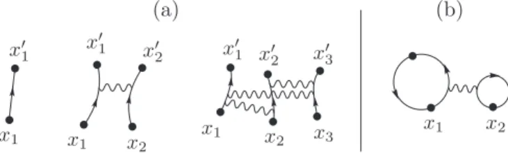
In order to calculate thermodynamic quantities or reduced density matrices one has to (partially) trace the N-particle propagator. Already for moderate particle numbers this leads to a plethora of identical contributions in Eq. (7) due to particle relabeling. This suggests a diagrammatic treatment of the (symmetry-projected) cluster expansion (7). Each interaction contribution of ordernis thus represented as a diagram con- nectingninitial andnfinal coordinates. The diagrams for the first three orders are displayed in Fig.1(a), where the particle coordinates are marked by labeled dots. Diagrams that appear

FIG. 1. (a) Diagrams representing K⁽ⁿ⁾(x,x;t), Eq. (6), for n=1,2,3. (b) Diagram representing the particular cluster Eq. (8) for x=x.

in (partial) traces are constructed from those building blocks. A full diagram represents a factorization into clusters according to Eq. (7) or its symmetry-projected equivalent and comprises several irreducible diagrams that represent single clusters. By convention each unlabeled bullet in a diagram stands for a coordinate that has been traced out. Such points have to be connected to two other points in the diagram. Loose ends are possible in general (for example, in off-diagonal elements of the one-body density matrix) but will not be important in this article. The irreducible diagram corresponding to Eq. (8) for x=xand withx₃traced out is depicted in Fig.1(b). In practice it is convenient to omit one-particle irreducible diagrams while stating the particle number of the reduced diagrams explicitly.

Let us now focus on diagrams that appear in the full trace of the cluster expansion, i.e., the partition function, with the purpose of counting only distinct diagrams, then provided with multiplicities. Consider a full diagram in the expansion that is built out ofl irreducible diagrams of sizesn₁· · ·nl. By distributing the particle indices among the irreducible diagrams in a different way one finds equivalent full diagrams. Therefore, the multiplicity of any such diagram contains the combinatorial factor

#^N_N= 1 _∞

ν=1m_N(ν)!

lN!

i=1ni!, (9) where m_N(ν) is the multiplicity of the number ν in N= {n₁, . . . ,n_l}. It is the number of possible partitions of theN particle indices into sets of the sizesn₁, . . . ,n_l. This holds ir- respective of the structure of the irreducible diagrams, whereas an additional factor counts the number of ways to relabel the coordinates inside an irreducible diagram depending on its structure. If we collect all full diagrams in the cluster expansion that factorize into irreducible diagrams of the sizesn₁, . . . ,n_l their sum can be written as

#_N^Nl

i=1

S_n⁽⁰⁾

i , (10)

where S_n⁽⁰⁾ is the sum of alln-particle irreducible diagrams, including the multiplicities from internal relabeling. As an example consider the cluster expansion for three bosons. There are three different partitions of the particles with combinatorial factors

#³_{1,1,1}=1, #³_{2,1}=3, #³_{3}=1 (11) so that the partition function is given by

Z= S₁⁽⁰⁾3

+3S₂⁽⁰⁾S₁⁽⁰⁾+S₃⁽⁰⁾. (12)

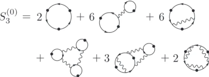
FIG. 2. The sum of irreducible three-particle diagramsS₃⁽⁰⁾. Most of the diagrams appear with multiplicities larger than 1. The first line includes only the interaction contributions up to order 2, while the second line accounts for all six possible permutations of the third- order interaction contribution. For distinguishable particles only the fourth diagram contributes.

The sum of the three-particle irreducible diagramsS₃⁽⁰⁾ with their individual multiplicities is shown in Fig. 2. Let us focus on the multiplicity of the second diagram. It is built from one interaction contribution of order two and one free propagation (order one). Choosing the interacting pair out of three particles already gives three possibilities corresponding to the Ursell decomposition, cf. Eq. (5). Then, one of the interacting particles has to be linked to the free particle by a permutation. This can be achieved with two distinct exchange permutations, yielding the overall multiplicity of 6. A detailed description of how the coefficients are determined in general can be found in [33].

When dealing withpartialtraces the combinatorial factors in Eq. (9) as well as the multiplicities of the irreducible diagrams with fixed coordinates have to be modified but the general statement remains.

C. The nonlocal pair correlation in cluster expansion We focus on the normalized nonlocal pair-correlation func- tion for bosons which, for a homogeneous system with fixed particle numberN, is defined as

g^(N)₂ (r)=ˆ^†(0) ˆ^†(r) ˆ(r) ˆ(0)

ρ² , (13)

where ˆ(x) and ˆ^†(x) are the bosonic field operators at position x and ρ=N/V is the particle density. By taking the expectation value in the canonical ensemble we can write Eq. (13) in terms of the many-body propagator

g₂^(N)(r)= 1 ρ²

N(N−1) Z₊^(N)

×

d^N−2xK₊^(N)(x,x;t = −ihβ)¯ |x₁=0,x2=r (14) with the canonical partition function

Z₊^(N) =

d^NxK₊^(N)(x,x;t= −ihβ).¯ (15) A derivation can be found in Appendix A. In the presence of external potentials the normalization has to be replaced according toρ² →ρ(0)ρ(r). Both numerator and denominator in Eq. (14) can now be expanded in terms of cluster diagrams.

Let us define S_n^(k)(x₁, . . . ,x_k|x1, . . . ,xk) as the sum of all

n-particle irreducible diagrams (including multiplicities from internal relabeling) that have all butkcoordinates traced out.

It is usually more convenient to work with the rescaled cluster sums

B_n^(k)≡ S_n^(k)

(n−k−δ_k0)!, (16) where the factorial accounts for the multiplicity of the cycle diagrams in the noninteracting case andδ_k0is the Kronecker δ. The functionsB_n^(k)are recursively related to each other by

dxk+1B_n^(k+1)(x₁, . . . ,x_k,xk+1|x1, . . . ,xk,xk+1)

=(n−k−δ_k0)!

(n−k−1)! B_n^(k)(x₁, . . . ,x_k|x₁, . . . ,xk). (17) With these definitions we can partially factorize the cluster expansion similar to Eq. (10), but we have to distinguish the case where the fixed coordinates x₁ and x₂ belong to the same irreducible diagram from the case where they belong to different ones. Making use of the cluster expansion of the partition function leads to the general result

g₂^(N)(r)= 1 ρ²Z^(N)

_N

k=2

B_k⁽²⁾(0,r)Z^(N−k)

+

N−1 k=1

N−k l=1

B_k⁽¹⁾(0)B_l⁽¹⁾(r)Z^(N−k−l) , (18) where we use the shorthand notationB_k⁽²⁾(x,y)≡B_k⁽²⁾(x,y|x,y) andB_k⁽¹⁾(x)≡B_k⁽¹⁾(x|x) and omitted the index+in the partition functions as this (purely combinatorial) result is not restricted to bosons. The partition function can be conveniently calcu- lated from the recursion relation

Z^(N)= 1 N

N k=1

B_k⁽⁰⁾Z^(N−k) (19) that stems from purely combinatorial calculations, too. In both Eqs. (18) and (19) we have definedZ⁽⁰⁾=1.

D. Short-time approximation

Up to this point the expression forg^(N)₂ is exact but purely formal. A key step now is to realize that for temperatures above the quantum degenerate regime it is sufficient to include short-time information on the propagatorsK⁽ⁿ⁾to be specified in the following. For finite systems without external potentials we replace all the propagators in the calculation by their infinite space equivalents, i.e., we assume that the particles do not explore the whole system in arbitrarily short times.

The condition for this approximation to be accurate can be estimated at the single-particle level to be

t mV^D2

2πh¯ ≡t_T, (20)

where mis the mass of the particle, V is the volume of the system, and D is the dimension. The characteristic time t_T can be thought of as the typical traversal time through the system of a particle with momentum ¯hV^−1/D, where the latter corresponds to the minimal uncertainty in the momentum of a

wave packet in the volumeV. If we switch to imaginary time the condition (20) can be translated into

λ^D_T V , (21)

introducing the thermal (de Broglie) wavelength λ_T =

2πh¯²β

m . (22)

At this length scale the propagator of a single free particle decays in imaginary timet= −ihβ. This gives the intuitive¯ picture that within the regime of validity of the short-time approximation all clusters of particles have a characteris- tic size that scales with λT that is much smaller than any length scale introduced from external confinement, such that their internal structure is essentially independent of the latter.

We have to stress that the short-time approximation does not require that the thermal wavelength be small compared to the mean interparticle separation, i.e., we can have

N λ^D_T

V >1, (23)

in contrast to the case of high-temperature expansions in the thermodynamic limit.

In the presence of smooth external potentials the short-time approximation can be modified such that only the internal dynamics of a cluster is mapped to infinite space, while its center of mass evolves according to the single-particle (short- time) propagator [34].

The short-time approximation defined above is well known in semiclassical physics, where it corresponds to taking into account only the shortest classical paths in the Van Vleck–

Gutzwiller propagator [35]. It can thus be easily extended to include, e.g., corrections from boundaries, which has its direct application in the calculation of the mean density of states, known as Weyl’s law [32]. The short-time approximation of the propagator thereby encodes the information on the slowly varying parts of the density of states. Note that the bound in Eq. (20) plays the role of a Heisenberg time t_H=2πh/,¯ where is the mean single-particle level spacing. It can be understood as a lower bound for the time needed to resolve the discreteness of the spectrum. This means that the price we pay for using the short-time approximation is the loss of all information related to this discreteness.

The power of the short-time approximation lies in the high level of generality leading to certain general scaling properties. We first focus on the full trace of a cluster as it appears, e.g., in the partition function. For homogeneous systems the short-time approximation tells us that, due to translational invariance, every cluster contributes with a factor proportional to the volume of the system (the presence of smooth external potentials results in an effective volume [34]).

ForD-dimensional homogeneous systems this will lead to a volume factorV for every fully traced cluster. Now we assume an interaction potentialUthat depends only on the coordinates x, an interaction parameterαwith the dimension of energy, and the physical constantsmand ¯h. A dimensional analysis then shows that we can write the potential asαU(˜ √

¯

αx/λT) in terms of a dimensionless function ˜U(y), a dimensionless parameter

¯

α=βα, andλT. Using this scale transformation we can rewrite

the interaction contributions

K⁽ⁿ⁾(x,x;t = −ihβ)¯ =λ⁻_T^nDK˜⁽ⁿ⁾ x

λT

, x λT

; ¯α

(24) as a dimensionless functionK˜⁽ⁿ⁾. This implies very generally that in the short-time approximation the functions B_n^(k) in Eqs. (16)–(19) will be proportional to λ⁻_T^kD for k >0 or to V /λ^D_T for k=0. To make this explicit we define the dimensionless functions

b^(k)_n =λ^kD_T B_n^(k) fork >0, b⁽⁰⁾_n = λ^D_T

V B_n⁽⁰⁾, (25)

that only depend on rescaled variables such asx/λT and ¯α. A direct implication is that the nonlocal pair-correlation function g₂^(N)(r) can be written as a rational function in the parameter V /λ^D_T with coefficients that depend only on the functionsb^(k)_n (withk=0,1,2). The partition function takes the form of a polynomial inV /λ^D_T with coefficientsb⁽⁰⁾_n , whereas the factor ρ⁻²∝V²compensates for the missing volume dependence in the numerator of the cluster expansion (18) forg₂^(N).

III. APPLICATION TO LIEB-LINIGER GAS A. The model

We now apply the methods of the previous section to compute the pair correlation for the case of N bosons with repulsive short-range interactions in a 1D ring geometry. We describe this system by the well-known Lieb-Liniger (LL) model defined by the Hamiltonian [20,36]

Hˆ = h¯² 2m

⎛

⎜⎜

⎝ N

i=1

− ∂²

∂xi2 +c N

i,j=1

i=j

δ(xi−xj)

⎞

⎟⎟

⎠, (26)

with c0, xi ∈[−L/2,L/2], where L is the system size, and periodic boundary conditions. The relevant dimensionless coupling parameter in the weakly degenerate regime is cλ_T. The symmetric eigenfunctions of the Hamiltonian (26) can be found via a Bethe ansatz, where periodicity leads to a quantization condition in terms ofN coupled transcendental equations [20].

In the limitL→ ∞, sometimes referred to as extended LL model, the spectrum becomes continuous. The symmetrized many-body propagator for this extended system is known ex- actly from integrating over all Bethe ansatz solutions [37–39].

We were able to rederive this propagator using the closed-form expressions for the wave functions introduced in [36] to get the strikingly simple form

K₊^(N)(x,x;t)= 1 N!

P∈SN

K¯^(N)(Px,x;t) (27) with

K¯^(N)(x,x;t)= 1 (2π)^N

d^Nk e^{−i2mht¯ k2+ik(x−x)}

×

j >l

kj −kl−icsgn(x_j −x_l) kj−kl−icsgn(xj −xl). (28)

A derivation of this result can be found in Appendix B.

Note that the function ¯K is not the many-body propagator for distinguishable particles but can be used as a substitute in the cluster expansion for bosons. Since only symmetry- projected quantities matter, eventually we are free to replace the interaction contributions K⁽ⁿ⁾ in the Ursell decomposition (7) by their symmetry-projected equivalentsK₊⁽ⁿ⁾. The corre- sponding expressions forn=2,3 can be found in AppendixC.

The nonsymmetrized expression forK⁽²⁾can be calculated from the propagator for a δ potential directly, which gives exactly the same result, as it is already symmetric with respect to particle exchange (antisymmetric states are not affected by theδpotential). The corresponding derivation can be found in AppendixC.

B. Lieb-Liniger model for three particles—Full cluster expansion

We will first address the full cluster expansion forN =3 particles calculated from the propagator (28). As discussed in Sec. II D, it comes as a rational function in L/λT with coefficients that are dimensionless functions of the rescaled quantitiesr/λ_Tandcλ_T. Due to the homogeneity of the system the diagonal part ofb⁽¹⁾_n does not depend onr, leading to the identification

b⁽¹⁾_n (r)=b⁽⁰⁾_n ≡b_n. (29) By expanding the general result forg₂^(N), Eq. (18), with the help of Eq. (19) forN=3 and using the shorthand notation b⁽²⁾_n (r)=b⁽²⁾_n (0,r) we can write the nonlocal pair-correlation function as

g₂⁽³⁾(r)=2

3 ×1+

b⁽²⁾₂ (r)+2b₂^λ_L^T

+b⁽²⁾₃ (r)^λ_L^T 1+3b2λT

L +2b3

_λT

L

2 . (30) We have calculated the functionsb⁽²⁾_n (r) andbnfor n=2,3 from the interaction contributionsK₊⁽²⁾andK₊⁽³⁾. Forn=2 we get the simple result

b⁽²⁾₂ (r)=e^−˜r2 1−√

4πc e˜ ^{( ˜c+|˜r|)2}erfc( ˜c+ |˜r|)

, (31) b₂= 1

√2

2e^c˜2erfc( ˜c)−1

, (32)

where ˜r=√

2π r/λT is the distance in terms of the thermal wavelength and

˜

c=λTc/√

8π (33)

is the dimensionless (thermal) interaction strength. The cor- responding expressions for n=3 are more complicated and can be found in AppendixC, Eqs. (C7)–(C9), and Eq. (C12).

The integrated functionb₂in Eq. (32) is closely related to the virial coefficient found in [40] for the spin-balanced Gaudin- Yang model. The correct normalization

dr g₂⁽³⁾(r)=2L/3 is obtained from Eq. (17) only if the integration domain (−L/2,L/2) can be replaced byRin all nontrivial integrals in the spirit of the short-time approximation, i.e., ifb⁽²⁾_2,3(r)≈0 for|r|> L/2. In the case at hand this gives the natural bound

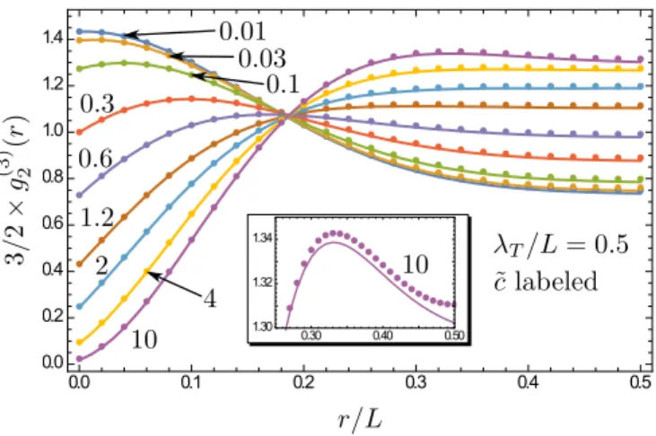
FIG. 3. Comparison ofg₂⁽³⁾(r), Eq. (30), (solid lines) with nu- merical calculations (dots) forλT/L=0.5 and various values of the thermal interaction strength ˜c, Eq. (33) (labeled). The inset shows the maximum arising for ˜c=10, an indicator of quasicrystalline order.

λT L/2 for the short-time approximation to be valid as both b_2,3⁽²⁾ have a typical extent of λT. This means that we can make predictions for very low temperatures as long as the semiclassical result forg^(N)₂ (r) saturates well beforer=L/2.

For comparison with numerical results we calculated the exact correlation function using the Bethe ansatz solutions similar to [23]. The details can be found in AppendixD. It is straightforward to show that the system sizeLcan be elimi- nated completely fromg₂in both results using the scale trans- formationx_i →x_i/L, k_i →k_iL, c→cL, β→β/L², where thek_iare the quasimomenta that appear in the Bethe solutions.

We thus express r and λT in units of L in all plots and use λT as the temperature parameter rather than T or β. Figure3 shows 3/2g₂⁽³⁾(r) for various values of ˜c, Eq. (33), and for λT/L=0.5. The absolute and relative error in the semiclassical results are smaller than 10⁻² for all values of ˜c at this temperature. For higher temperatures the results are more accurate, e.g., for λT/L=0.3 (not shown) both the absolute and relative error of the semiclassical result are of the order 10⁻⁶ for all values of ˜c. Considering the fact that forλT/L=0.5 the numerical calculations converge up to an error of 0.1% already for a summation cutoff after only 15–30 states (depending on the interaction strength), the accuracy of the semiclassical prediction based on a continuous spectrum is impressive.

Interestingly, a feature that usually becomes visible only for very low temperatures, the nonmonotony of g^(N)₂ in the fermionization regime of large ˜c[27,41], can already be seen in Fig.3. There, the maximum value ofg⁽³⁾₂ (r) atr/L≈1/3 for ˜c=10 is highlighted in the inset and can be interpreted as a precursor of a quasicrystalline order in the two-particle correlations. For larger values ofλT >0.5Lthe approximation fails as expected.

C. Exploiting the universal scaling of the short-time approximation

The general scaling properties of the short-time approxima- tion that we found in Sec.II Dare not only useful to identify

FIG. 4. The nonlocal pair-correlation function for N=5 par- ticles from Bethe ansatz calculations (dots) and the semiclassical result (solid lines) forλT/L=0.4 using the functionsb⁽²⁾_n (r) andb⁽⁰⁾_n Eq. (25) forn=4,5 that have been recursively extracted from the numerical results forg₂⁽⁴⁾(r) andg₂⁽⁵⁾(r) atλT/L=0.1. The values for

˜

c(ranging from 0.01 to 10, from top to bottom atr=0) are the same as in Fig.3.

relevant parameters of the theory but can actually be used as a predictive tool. Let us assume that we know the expressions for bnandb⁽²⁾_n (r) up to a certain cluster sizen=l−1. If we can find, in whatsoever way, e.g., by direct measurement [11], an expression forg₂^(l)(r) for fixed values of ˜cand (small enough) λ_T it contains all the information we need to calculateb_land b_l⁽²⁾(r). The scaling behavior of the latter can then be used to calculateg^(l)₂ (r) at all temperatures in the range of validity of the short-time approximation with the same ˜cor to find better approximations for higher particle numbers (see next section). The interplay between the scaling of the functions b_n^(k)and the form ofg^(N)₂ as a rational function inλT/Lrenders this approach nontrivial. To actually calculateb⁽²⁾_l andblfrom g^(l)₂ , we note thatb⁽²⁾_n (r)→0 forr → ∞and that the cluster expansion ofg₂^(l) containsbl only in the denominator. This means thatg₂^(l)(r)/g^(l)₂ (∞) depends onb_l⁽²⁾(r) but not onbl, while the latter can be found independently fromg^(l)₂ (∞). In practice, the diverging argumentr→ ∞has to be replaced by a value that lies inside the saturation regime ofg₂^(l). This explains why we have to knowg₂^(l)(r) for “small” values ofλ_T. As the above considerations use only the homogeneity of the system, they are not restricted to 1D or toδ-like interaction potentials.

To demonstrate the power of the method, we have used the numerical results from the Bethe ansatz calculations ofg₂⁽⁴⁾(r) andg⁽⁵⁾₂ (r) atλ_T =0.1Land various values of ˜cto calculate the clusters b_n⁽²⁾ andb⁽⁰⁾_n for n=4,5. The results have then been used to calculateg₂⁽⁵⁾(r) atλT/L=0.4. The comparison of the respective predictions with the numerical calculations is shown in Fig.4. The nearly perfect agreement for all values of the interaction strength shows that the method is indeed applicable to the case at hand.

We have investigated the breakdown of the validity of our approach by calculating the mean absolute error in the

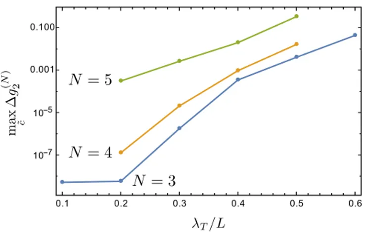
FIG. 5. The maximum (with respect to the interaction strength ˜c) of the mean difference between semiclassical and numerical results (see text). While the deviation is smaller than the numerical precision forN =3,λT 0.2 it increases rapidly forλT/L0.2.

semiclassical results forg^(N)₂ (r) using the 2-norm

g^(N)₂ =

1 λT

λ_T 0

dr

g₂^(N)(r)2

, (34)

where g₂^(N)(r) is the difference between the numerical and semiclassical results. Figure 5 shows the maximum of this mean error with respect to the interaction strength ranging from 0.01 to 10 forN=3,4,5 and for various values ofλ_T/L. For N =3 andλ_T 0.2 the error is smaller than the numerical precision (see AppendixD). The deviation forλT =0.1Lis not shown forN =4,5, as this is the value used for the extraction of the functionsb⁽⁰⁾_n ,b⁽²⁾_n (r) forn=4,5. The large offset between the graphs for the different particle numbers can be explained by the rather small numerical precision in the extracted cluster contributions, but all three curves show a roughly exponential increase in the range of 0.1λT/L0.5, indicating a sudden breakdown of the short-time approximation.

D. Truncated cluster expansion for higher particle numbers The full cluster expansion for g₂, in principle, could be calculated from the propagator (28) for arbitrary particle numbers N. In practice one would have to (partially) trace not onlyK⁽ⁿ⁾for 1nN, which is a difficult task, but also all permutations of different products thereof. Here we will use only the information from interaction contributions up to third order. One way to achieve this goal is to truncate the expansion into interaction contributions, Eq. (7), to take into account only the desired orders. This has been proven to yield excellent results for the canonical partition function with a truncation to second-order interaction contributions [34]. The resulting expressions comprise clusters of all sizes due to the symmetrization of the propagator. But already at the level of cluster sizesn3 we can make good predictions for certain regimes while using only such minimal information. As argued above, the full cluster expansion is a rational function in the parameterλT/Lwith coefficients that are functions of ˜r,c, and˜

N. WithAn(r)=b_n⁽²⁾(r)−(n−1)bnλT/Lwe can writeg₂as

g^(N)₂ (r)= N−1 N

1+A₂(r)+_N−2

1

A₃(r)+_N−2

2

b₂A₂(r)_λ

T

L +O(2) 1+_N

2

b₂^λ_L^T +O(2) , (35) whereO(2) stands for higher orders inλT/L. We can now expand this function into a formal series in the parameterλT/L, while treating the functionsAnas constants to preserve normalization. This results in

g₂^(N)(r)≈ N−1 N

1+A₂(r)+[(N−2)A₃(r)−(2N−3)A₂(r)b₂]λT

L

. (36)

The terms of orderninλT/Lnow come with a polynomial in the particle numberN that is of the ordern, a fact that is well hidden in the rational expression forg₂^(N). The series expansion has a positive convergence radius for any finite particle number, and the truncation is a good approximation if we take the ratio between the thermal wavelength and the mean interparticle distance,

n_T =N λ_T/L, (37) as a small parameter. Figure 6 shows the comparison of Eq. (36) with numerical calculations forN =5 particles and N λT/L=0.5. The agreement is very good for the whole range of interaction parameters ˜c. The inset shows the effect of truncating the expansion Eq. (36) to single two-particle clusters (first two terms in the equation) and the effect of neglecting terms of subleading order in the particle number, respectively, for ˜c=0.3 (the latter corresponds to the thermodynamic limit that will be addressed below). Clearly, there is a major improvement by using the additional information from b⁽⁰⁾₃ , b⁽²⁾₃ (r), and multiple clusters, where finite-size effects play a crucial role. Also note that the fermionic limit ˜c→ ∞atr=0 yields zero for all orders in the full expansion, which is often

FIG. 6. Comparison of the expansion for g₂⁽⁵⁾, Eq. (36), with numerical results (dots) forλT/L=0.1 for the same range of values of ˜cas in previous figures. The inset shows the effect of truncating the expansion ofg⁽⁵⁾₂ after the single two-particle clusters [first two terms in Eq. (36)] (triangles) and the effect of neglecting all coefficients that are subleading in the particle number (squares), i.e., Eq. (38), for

˜ c=0.3.

referred to as antibunching. Thus, in this limit the error in the truncated expansion (36) is of the ordern²_T/N.

E. The thermodynamic limit

From the virial-like expansion Eq. (36) it is easy to find the thermodynamic limit by omitting all terms that are subleading inN while fixingnT, Eq. (37). This gives

g₂(r)=1+b⁽²⁾₂ (r)+

b⁽²⁾₃ (r)−2b2b⁽²⁾₂ (r)

nT +O n²_T

. (38) Equation (38) can also be found within a grand-canonical approach by inverting the fugacity expansion in terms of the particle number in the high-temperature limit [33]. A comparison with numerical results obtained in [27] is shown in Figs. 7 and 8. Figure 7 demonstrates the validity of our result in the full range of interactions. For high temperatures (low densities)nT 1 it suffices to take into account only b₂⁽²⁾(r). For higher values of nT the next-order term gives non-negligible corrections. Figure 8 shows g₂(r) for nT =

√π/2500,√ π/25,√

π/2.5 and ˜c²=0.18,0.1568,0.1125, re- spectively. For n_T =√

π/2500, g₂ can be approximated by single- and two-particle clusters. For higher values ofn_T the O(nT) contributions, and thus three-particle clusters, have to be included, and fornT =√

π/2.5≈1.12 the truncation to first order innT is not sufficient anymore for a precise prediction but still gives reasonable qualitative agreement with numerical calculations. Figure 9 shows the local correlationsg₂(0) for

FIG. 7. Comparison of numerical results forg2(r) from [27] (for error estimates see [27]) with Eq. (38) fornT ≈0.035 and ˜clabeled.

The numerical method in [27] cannot access the fermionization regime ˜c1.

FIG. 8. Nonlocal pair correlation in the thermodynamic limit for different interaction strengths and different values ofnT such that g2(0)≈1. In the high-temperature or low-density regimenT 1 only two-particle clusters contribute. For lower temperaturesO(nT) corrections cannot be neglected and larger clusters play a role.

a wide range of the interaction parameter. By including the first-order correction innTwe can see a major improvement in the agreement of numerical (taken from [42]) and semiclassical results. Note that the local versiong₂(0) of the pair correlation can be calculated exactly by solving integral equations using the Hellmann-Feynman theorem [42] (higher local correlation functions have been found from viewing the LL model as a limiting case of the sinh-Gordon model [43]), but to the best of our knowledge, all published analytical results forg₂(r) in the weakly degenerate regime were derived in perturbation theory, i.e., they are only valid in the limits of weakly or strongly interacting bosons. Our result, Eq. (38), represents the generalization of these results for arbitrary interaction strengths in the moderate- to high-temperature regime.

FIG. 9. Local correlationsg2(0) with respect to the interaction parameter. Numerical data (dots) is taken from [42]. The approx- imation by two-particle clusters (gray dashed) is sufficient for high temperatures (low densities). By including the next order in the cluster expansion (solid line) we can see a major improvement in the regime of lower temperature.

IV. CONCLUSION AND SUMMARY

In this paper we have addressed the spatial structure of few- and many-body states in interacting quantum systems by means of the nonlocal correlation functions. Using a combination of two key ingredients, namely, neglecting the discreteness of the extremely dense many-body spectrum and including interaction effects nonperturbatively by means of cluster expansions, we derived analytical formulas for two- point correlators covering a wide range of temperatures and interaction strengths.

Specifically, by making use of the method of Ursell op- erators we developed an exact formula for the nonlocal pair- correlation function and the partition function for finite particle numbers in terms of sums of irreducible (cluster) diagrams. We then showed how, in the high-temperature regime λ^D_T V, these diagrams can be calculated from semiclassical short- time approximations of the quantum-mechanical many-body propagators. We used these methods to calculate explicit ana- lytical formulas for the nonlocal pair-correlation function in the Lieb-Liniger gas for temperatures above quantum degeneracy that we compared with numerical calculations based on the exact Bethe ansatz solutions of the model. For the example of three particles we showed that the full cluster expansion in short-time approximation remains valid up to λ_T ≈L/2.

We then demonstrated that the universal scaling behavior of the latter remains valid for higher particle numbers. This was done by predicting the form of the nonlocal pair-correlation function for a whole range of temperatures by rescaling the numerical values for a fixed temperature. Comparing the results obtained from this rescaling procedure to numerical calculation showed very good agreement down toλT =0.4L.

For higher particle numbers we presented approximations that are valid well above the quantum degeneracy regime, i.e., N λT/L1, while still explicitly depending on the particle number and thus explicitly accounting for its finiteness. Finally, by neglecting the contributions that are subleading in the particle number, we presented the exact results for the first two orders of the series expansion of g₂(r) in the quantum degeneracy parameternT =N λT/Land showed that it agrees well with the numerical results that were obtained by other authors. While our work awaits experimental confirmation in state-of-the-art experiments with 1D trapped quantum gases in the weak degeneracy regime, we plan to extend our analysis to momentum correlations in the 1D Bose gas that have been measured recently [44].

ACKNOWLEDGMENTS

B.G. thanks the Studienstiftung des deutschen Volkes for support. We further acknowledge financial support through the Deutsche Forschungsgemeinschaft (through SFB 1277, Project A07). We thank Piotr Deuar and Peter Drummond for providing the numerical data from Ref. [27].

APPENDIX A: PAIR-CORRELATION FUNCTION IN THE CANONICAL ENSEMBLE

To derive Eq. (14) from (13) we perform the trace inO = Tr^(N)₊ {e^−βHˆO}/Z^(N)₊ in the position basis of the Hilbert space