12 Atmospheric Dispersion Modelling

- 1 -

12 Atmospheric Dispersion Modelling

12.1 Overview

If any trace gas or ‘pollutant’

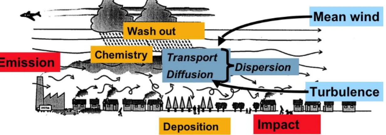
is emitted into the ABL it will undergo various processes that all together eventually lead to a concentration distribution somewhere downwind of the source. Figure 12.1 sketches these processes indicating the complicated interactions between various stages of the chain.

Basically, we discriminate between the action of the mean flow (‘transport’) and that of turbulence (’turbulent diffusion’) which together lead to what is called dispersion. Generally, in atmospheric dispersion modelling it is assumed that the pollutant has the physical properties of air (i.e., the molecular weight of essentially a mixture between O

and N

). This is justifiable if it is a gaseous compound

or even a small aerosol. However, if the pollutant is solid and has a non-negligible size (an arguable ‘limit size’ is PM10, i.e. a particle size of less than 10 microns) at least one additional process becomes important, namely sedimentation.

Figure 12.1 Schematic representation of processes contributing to the fate of atmospheric pollutants from the emission to the impact.

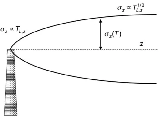
An idealized picture of the concentration distribution downwind of a source is that of a plume (Fig. 12.2). This is the concentration distribution that would evolve in a horizontally homogeneous, stationary boundary layer (with non- negligible mean wind). These two strong assumptions of course lead to a considerable simplification of the dispersion problem, so that theoretical predictions are possible. For a considerable part of the (early) twentieth century, therefore, dispersion modelling was essentially plume modelling.

Taylor’s plume theory set the stage by using basic principles on turbulence

1

We do not distinguish here any possible adverse effects of the released ‘trace gas’ in principle, only its physical properties and the related process of dispersion. Clearly, however, it is of much greater interest to understand these processes if the trace gas is not simply a noble gas or any other harmless substance.

2

Even if the molecular weight should be much larger than, as it is the case for example for

CO

or even heavier gases.

statistics in order to predict the overall growth of a plume as a function of travel time. It will be discussed in the next section. Here, we only start by introducing the descriptors of a plume. While a plume is often visible (hence probably its ‘success’ as a concept in dispersion modelling) the actual concentration of the tracer is ‘somehow’ distributed around a centre of gravity of its mass. Most conveniently this distribution is assumed to be normal (Gaussian) and the plume size is characterised by the standard deviation of the (normal) mass distribution (Fig. 12.2). Standard notation uses

€

σ

for the plumes vertical extension (as seen from the side) and

€

σ

for the plume width (as seen ‘from above’). These two ‘sigmas’ characterising the plume must not be mixed with the standard deviation for the vertical and lateral wind components,

€

σ

and

€

σ

, respectively. The most probable concentration or centre of gravity of the plume in the vertical is denoted

€

z and (if the model allows for horizontal inhomogeneity)

€

y for its lateral position.

Figure 12.2 Sketch of a plume with the mean ‘plume height’,

€

z , and plume spread,

€

σ

.

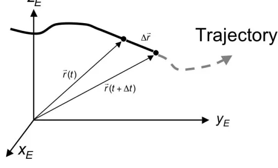
To understand different types of atmospheric dispersion models it is necessary to introduce two fundamental frames of reference, in which fluid dynamics problems can be addressed. Both are named after famous mathematicians, the Swiss Leonhard Euler (1 7 0 7 - 1 7 8 3 ) and the

3

Note that here the more common σ

, σ

is utilized, rather than σ

,σ

2

as in the rest of

this text.

- 3 -

Italian/French Joseph Louis Lagrange (1736–1813, born Giuseppe Lodovico Lagrangia in Turin, Italy) . The more familiar of the two is the Eulerian frame of reference. This is fixed in space with a specified origin. Whether this is a Cartesian coordinate system as in Fig. 12.3 or any other is not essential.

Usually, in this frame of reference, the problem of atmospheric dispersion is addressed by solving the conservation equation for mass (of the tracer to be dispersed). This can be done either by simplifying to a degree that the equation has an analytic solution (see Chapter 13) or by means of numerical modelling, i.e. by numerically solving the equation on a grid. The Eulerian frame of reference is advantageous if many sources are to be treated or if a numerical model is available anyhow.

A Lagrangian frame of reference is a way of looking at fluid motion where the

‘observer’ follows individual fluid particles as they move through space and time. Plotting the position of an individual particle through time gives the path line of the particle (Fig. 12.3). This might be visualized by sitting in a boat drifting down a river. With respect to dispersion modelling this means that

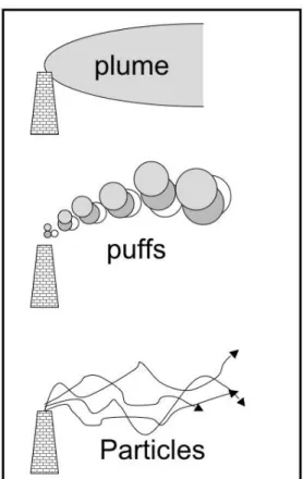
‘travel time’ becomes the variable of interest, indicating how much dispersion will have occurred since the time of the release from the source. If a plume model is formulated with respect to (travel) time, it is essentially Lagrangian in nature. A more sophisticated method of describing the evolution of pollutant plume is the puff model where a series of puffs is emitted from the source and their growth is modelled as they travel down wind (Fig. 12.4). In the case of an ideal horizontally homogeneous and stationary situation, the sequence of puffs, of course, will simply make up the plume. The most advanced of the Lagrangian dispersion models, finally is the so-called Lagrangian particle dispersion model. Here thousands of individual particles (fluid elements) are traced and their distribution yields an estimate for the concentration field.

Figure 12.3 Lagrangian trajectory in an Eulerian co-ordinate system.

Figure 12.4 Different types of atmospheric dispersion models: plume models (top), puff models (middle) with different shading indicating different release times for the growing puff, and particle models (bottom).

12.2 Statistical Theory of Taylor

The goal of P.A. Taylor’s analysis (Taylor 1921) is the theoretical description of the growth of a plume under stationary and horizontally homogeneous conditions. Often, only the result is provided in textbooks (eq. 12.6), but due to its fundamental importance for the understanding and assumptions usually made in applied dispersion modelling a brief outline of its derivation is given here. The example is given for the lateral spread of the plume. Starting point is therefore the Lagrangian auto-correlation function (see eq. 3.27 for its definition) for the lateral velocity component:

€

R

(τ ) = v'

(t) ⋅ v '

(t + τ )

v'

^(12.1)

Here, ‘t’ denotes time,

€

τ a time difference and ‘L’ refers to ‘Lagrangian’. It is therefore explicitly stressed that

€

v

is the Lagrangian (lateral) velocity component. Due to stationarity, the velocity variance is independent of time.

We therefore can rearrange (12.1) and integrate with respect to time

difference τ ^:

- 5 -

€

v'

R

( τ ^')

0 τ

∫ d τ ^' = v '

(t) ⋅ v '

(t + τ ^')

0 τ

∫ d τ ^'

= v'

(t) v'

(t + τ ')d τ '

0 τ

∫

(12.2)

In (12.2) we have implicitly assumed that all the ‘fluid elements’ have started in a single point at

€

τ = 0 . The integral in the second line of (12.2) corresponds to the mean lateral distance,

€

Y , a fluid element has travelled during the time

€

τ . Therefore,

€

v '

(t) v '

(t + τ ')d τ '

0 τ

∫ = v '

Y (t, τ ) = v '

Y ( τ ) , (12.3) (the last equality due to stationarity). The variance of the lateral distance,

€

Y

, is – for a situation in which all the fluid elements start in

€

y = 0 at the time

€

t = 0 - nothing else than the plume width,

€

σ

. And due to stationarity this is true for any starting time

€

t . The time derivative of

€

Y

obeys

€

d

dt Y

= 2Y dY

dt = 2 Yv

, (12.4)

Combining (12.4), (12.3) and (12.2) leads to a new equation that relates the time derivative of

€

Y

with the lhs of (12.2). Integration with respect to (travel) time yields

€

2v'

0 T

∫ R

( τ ')

0 τ

∫ d τ 'dt' = ( d

0

dt

T

∫ Y

)dt ' (12.5)

Thus the final result that is usually referred to as the Theory of Taylor reads

€

2 v '

dt '

0 T

∫ R

( τ ^')

0 τ

∫ d τ ^' = σ

(T) [= Y

(T )] (12.6a)

Analogously, for the vertical direction the result reads

€

2w'

dt '

0 T

∫ R

( τ ')

0 τ

∫ d τ ' = σ

(T) [= Z

( T )] (12.6b)

In the limit of small travel times, i.e. close to the source, the auto-correlation function is approximately one and therefore

Small T:

€

σ

( T ) = v '

T

€

σ

( T ) = w'

T

(12.7) On the other hand, for large

€

t the integral of the auto-correlation function is defined as the (Lagrangian) integral time scale (3.29) and hence

Large T:

€

σ

( T ) = 2v '

T

T

€

σ

( T ) = 2w'

T

T (12.8)

The theoretical plume in stationary and homogeneous conditions therefore

grows proportional to travel time close to the source, and proportional to the

square root of travel time far away from the source (cf. Fig. 12.2).

Alternative formulation

For later use we look at an alternative formulation of the result from the Theory of Taylor (12.6), again on the example of lateral dispersion.

Partial integration of (12.6) yields

€

σ

( ) T ^{= 2v}

^∫ ( ^{T − τ} ) ^R

( ) ^{τ d τ (12.9)}

The auto-covariance function is the inverse Fourier transform of the spectral density function (see eq. 7.4)

€

R

( ) τ ⁼

^{∫ S}

( ) ^{n cos(2 π n τ )dn (12.10)}

where

€

n denotes the natural frequency and we have used the symmetry of the auto-correlation function

€

R ( ) τ ^{= R} ( ) ^−τ

( ) combining (5.12) and (5.13) yields

€

σ

( ) T ^{= 2v}

^∫ ( ^{T − τ} )

^{∫ S}

( ) ^{n cos(2 π n τ )dnd τ (12.11)}

since the Fourier integral is convergent the order of integrations can be inverted:

€

σ

( ) T ^{= 2v}

^{∫ S}

( ) ^{n } _ ^

^∫ ( ^{T − τ} ) ^{cos(2 π n τ ) d τ } _ ^{ dn (12.13)}

Partial integration of the square brackets yields

€

T − τ

( ) ^{cos(2πnτ )dτ}

0 T

∫ = − cos 2πnτ ( )

( ) 2πn







 







 

T

(12.14)

and therefore

€

σ

( ) T ^{= 2v}

^{∫ S}

( ) ^{n 1− cos(2πnτ} ₍₂ ⁾

π n)

dn (12.15)

This expression can finally be re-organised to read

€

σ

( ) T ^{= T}

^v

^{∫ S}

( ) ^{n  sin(} _(πnT ^{π nT} ₎ ⁾

 



 

2

dn (12.16)

This formulation for the Theory of Taylor using the spectral density function

will be used in the following when investigating semi-empirical methods to

describe the plume characteristics.

- 7 -

12.3 Semi-empirical Methods for the Plume Characteristics

According to the Theory of Taylor for stationary and homogeneous flows the plume characteristics,

€

σ

and

€

σ

, can be described as a function of the respective velocity variances and some other turbulence variables (either the auto-correlation functions or the integral time scales). However, immediate use of these relations is hindered by the fact that Lagrangian turbulence statistics are required in (12.6). These are, in general, quite difficult even to measure and thus parameterizations (see, e.g., Section 4.5.1 for the Surface Layer) are usually for Eulerian statistics

. The simplest way out would be to simply assume that Eulerian and Lagrangian velocity statistics are equal (i.e.,

€

u

= u

). This assumption would mean that averaging times are long enough to ensure that the Lagrangian ‘sampler’ encounters all the fluctuations, which are seen by a fixed (Eulerian) during a corresponding averaging period.

A less stringent assumption is to require that the Eulerian and Lagrangian auto-correlation functions are similar in shape (as observed, e.g., in one of the rare studies by Hanna (1981), see Fig. 12.5), but displaced by a factor

€

β ^:

€

R

( ) βτ ^{= R}

( ) ^{τ . (12.17)}

Here,

€

β is defined as the ratio of the integral time scales

€

β = T

T

^{. (12.18)}

From (12.17) it immediately follows that also the spectral functions are similar:

€

nS

( ) n ^{= β nS}

( ) ^{β n . (12.19)}

Figure 12.5 shows that indeed some similarity between the spectral functions seems to exist and that

€

β > 1 , i.e. the Lagrangian spectrum is displaced with respect to the Eulerian towards lower frequencies. Deeper analysis of spectra based on a simplified theory and some observations (Pasquill 1974) has shown that

€

β can be related to the turbulence intensity (eq. 3.26)

€

β = Dl

(12.20)

where

€

D ≈ 0.4 − 0.6 is an empirical parameter (with quite substantial scatter).

In order to find a general approach for the plume characteristics based on the Theory of Taylor, we first introduce a dimensionless time difference,

€

τ

= τ / T

(i=v,w) and introduce a dimensionless Lagrangian auto-correlation function

€

R

( τ

) assuming that within this scaling framework all auto- correlation functions should collapse into one single form (

€

R

( τ

)).

4

Note that in previous chapters the subscript ‘E’ has usually not been added even if all the

cited parameterizations refer to Eulerian statistics.

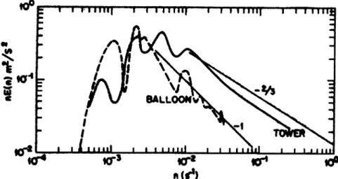
Figure 12.5: Lagrangian (‘balloon’) and concurrent Eulerian (‘tower’) energy spectra for the w component at a height of 300m (Hanna, 1982).

Consequently, a dimensionless spectral density function

€

S

(n

) is defined with the dimensionless frequency

€

n

= nT

. Finally, the dimensionless plume spread is defined according to

€

Σ

= σ

σ

T , (i, j) = (v,y) or (w,z) , (12.21)

and the dimensionless travel time is

€

T

= T / T

. In dimensionless form, then, the relation between plume spread and the turbulence characteristics due to Taylor’s Theory in its alternative form (12.16) becomes

€

Σ

= S

( ) n

^{sin πn}

*

⋅T

[ ]

πn

T















0



∞

∫

2

dn

^(12.22)

Equation (12.22) shows that the dimensionless plume spread is only a function of

€

T

if the dimensionless spectral density function is known:

€

Σ

= f

(T

), (i, j) = (v,y) or (w,z). (12.23)

The functions

€

f

are yet unknown and, of course, dependent on the spectral density function. However, from Taylor’s Theory we may assess their limits.

Equation (12.7), together with the definition of

€

Σ

(12.21) implies that Small T:

€

Σ

= 1 (12.24)

or

€

f

= 1 . Similarly, with (12.8) we find Large T:

Σ

= ( 1

2 T

)

(12.25)

- 9 - In between these two limits the functions

€

f

are dependent on the form of the spectral density functions. Overall, the relation between the plume characteristics and the turbulence statistics can thus be summarized (now again in dimensional form) as

€

σ

= σ

T ⋅ f

( T

T

), (i, j) = (v,y) or (w,z) (12.26)

Table 12.1 summarizes explicit formulations for the functions

€

f

for ground and elevated sources according to Gryning (1981). We first of all note that the limiting behaviour (especially for time going to infinity) is only loosely fulfilled in several cases. Also, for specific classes of spectra the dependence on the integral time scale vanishes. Overall, Table 12.1, together with (12.26) allows to determining plume characteristics under idealised conditions for simple plume model (Chapter 13).

Horizontal diffusion Vertical diffusion

stable unstable stable unstable

Ground sources T

= 300 s T

= 300 s T

= 50 s T

= 100s (T ≤ 550s) f

=(1) f

= (1) f

= (1) f

= (3)

(T ≥ 550s) f

=(2) Elevated

sources

T

= 1000 s T

= 1000 s T

= 100 s T

= 500 s f

= (1) f

=( 1) f

= (4) f

= (1) (1)

€

f

= 1

1 + 0.90( T T

)

(2)

€

f

= 1

1 + 28 T

(3)

€

f

= 0.3( T T

− 0.4)

0.16 + 0.7 (4)

€

f

= 1

1 + 0.945(T T

)

Table 12.1: Summary of

€

T

,

€

T

and equations for

€

f

and

€

f

, after Draxler (1976) (from Gryning 1981).

References

Draxler RR: 1976, Determination of atmospheric diffusion parameters, Atm Environ, 10, 99- 105.

Gryning, S.-E.: 1981, ‘Elevated Source SF6 Tracer Dispersion Experiments in the

Copenhagen Area’, Risø Report Risø-R-446, Risø National Laboratory, Roskilde, DK, 187 pp.

Hanna SR: 1981, Lagrangian and Eulerian time-scale relations in the day-time boundary

layer, J Appl Meteorol, 20, 242-249.

Hanna SR: 1982, ‘Applications in Air Pollution Modeling’, in: Nieuwstadt, FTM. and van Dop, H (Eds.), ‘Atmospheric Turbulence and Air Pollution Modelling’, Reidel, Dordrecht (358pp), 275-310.Hanna (1982)

Pasquill F: 1974, Atmospheric Diffusion 2

edition, John Wiley and sons, New York.

Taylor GI: 1921, Diffusion by continuous movements, Proc London Math soc, 20, 196-202.