Spatial patterns in shallow cumulus cloud populations over a

(1)

Spatial patterns in shallow cumulus cloud populations over a

heterogeneous surface

inaugural-dissertation

zur

Erlangung des Doktorgrades

der Mathematisch-Naturwissenschaftlichen Fakultät der Universität zu Köln

vorgelegt von

Thirza W. van Laar aus

Barneveld Die Niederlande

Köln 2019

(2)

Berichterstatter:

Prof. Dr. Roel A.J. Neggers Prof. Dr. Clemens Simmer

Tag der letzten mündlichen Prüfung:

22 July 2019

(3)

Rows and ows of angel hair And ice cream castles in the air And feather canyons everywhere I've looked at clouds that way But now they only block the sun They rain and snow on everyone So many things I would have done But clouds got in my way I've looked at clouds from both sides now From up and down, and still somehow It's cloud illusions that I recall I really don't know clouds at all Joni Mitchell - Both Sides Now

(4)

Abstract

Shallow cumulus clouds play an important role in the earth's climate. They are eective transporters of temperature, humidity and momentum and impact the radiation budget.

It is therefore important to correctly represent them in numerical weather prediction and climate models. However, because of their small scale they are not directly resolved by the large scale models. Their presence and eect therefore is approximated by parametrization schemes. These parametrization schemes use many assumptions and have their uncertainties, therefore clouds are one of the major sources of uncertainty for climate prediction.

To minimize the uncertainties associated with the dierent parametrization schemes, a more complete understanding of what inuences cloud formation is needed. In this thesis two specic aspects of processes associated with shallow cumulus cloud populations are studied. The rst one is their spatial organization. Through convective organization the mean state of the atmosphere is aected. Quantifying this behaviour could help in understanding the mechanisms behind organization. The second one is their dependence on surface conditions, more in particular the role of surface heterogeneity. Since shallow cumulus are strongly coupled to the surface, their formation and spatial distribution is inuenced by heterogeneous surface conditions. In this thesis rst some exploratory work is done on the description of a shallow cumulus cloud population in terms of size and spacing. The tools acquired are applied to asses the inuence of a heterogeneous surface on the spatial patterns in shallow cumulus cloud populations.

For a statistically reliable assessment of cloud size distributions, Large Eddy Simulations (LES) are used. 146 simulations are performed for days that feature shallow cumulus clouds. It is found that the cloud size distribution can be described by a power law- exponential function. The largest cloud in the eld is found to correlate with the total cloud cover, meaning that larger clouds contribute most to a larger total cloud cover, and not an increase in number of smaller ones.

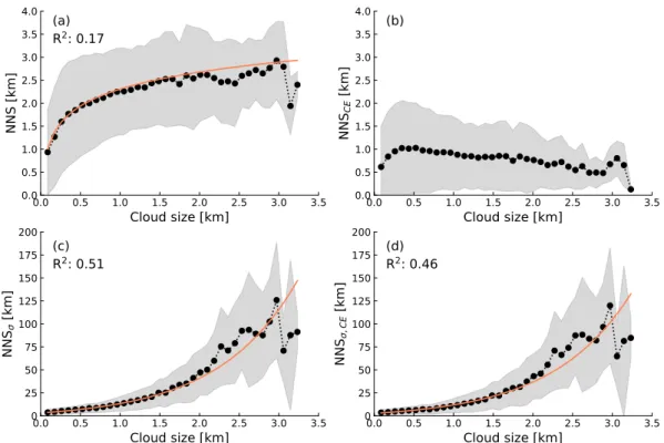
To study cloud spacing, data is used from a large domain LES over the ocean in the subtropics. The data shows that the more numerous small clouds surround larger ones.

The distances between clouds depend on the size of the cloud itself. The larger the cloud, the larger the distance to its nearest neighbor. The functional relation between cloud spacing and cloud size diers when either all clouds are taken into account, or only clouds of a similar size. For clouds of a similar size the spacing is found to increase exponentially with cloud size. To quantify the degree of organization of a complete cloud population, several parameters are evaluated. Taking into account advantages and disadvantages of all, it is concluded that Iorg is the best one to use, mainly because it describes the tendencies seen by eye and is useful over a range of scales.

Finally the impact of surface heterogeneity on the cloud population is studied. For this, two dierent shallow cumulus days are simulated using a realistic set-up with cloud resolving resolutions. A sensitivity study is done, increasing and decreasing the topography, and changing the distribution of land use types. The cloud size distribution is not greatly af- fected by these changes in surface conditions. The slope stays the same, only the maximum

(8)

cloud size diers slightly for the simulations, with the largest clouds for the simulations with increased topography. Judging by eye, the spatial distribution of clouds diers among the simulations, but this is not reected in Iorg. For the simulation with a dierent distribution of land use types a quasi secondary circulation can form if the wind direction allows for it. Even though quantication is not straightforward, using a realistic set-up shows that surface conditions do inuence the spatial patterns in shallow cumulus cloud populations.

(9)

Zusammenfassung

Flache Kumuluswolken spielen eine wichtige Rolle im Klimasystem. Sie transportieren Temperatur, Feuchte und Impuls und beeinussen die Strahlungsbilanz. Deshalb ist es wichtig sie korrekt in numerischen Wettervorhersage- und Klimamodellen zu repräsen- tieren. Allerdings werden sie aufgrund ihrer kleinen Skalen nicht direkt von den groÿskali- gen Modellen aufgelöst. Ihr Erscheinen und ihr Einuÿ werden deshalb durch Parame- terisierungen angenähert. Diese Parameterisierungen nutzen viele Annahmen und haben eigene Unsicherheiten, weshalb Wolken eine der Hauptquellen von Unsicherheiten in Kli- mavorhersagen sind.

Um die Unsicherheiten der verschiedenen Parameterisierungen zu minimieren wird ein um- fassenderes Verständnis der Einüsse auf die Entstehung von Wolken gebraucht. In dieser Arbeit werden zwei spezische Aspekte von Prozessen untersucht, die mit achen Kumu- luswolken Populationen verbunden sind. Der erste Aspekt ist die räumliche Organization.

Durch konvektive Organisation wird der mittlere Zustand der Atmosphäre beeinusst.

Dieses Verhalten zu quantizieren könnte helfen die Mechanismen hinter der Organisa- tion zu verstehen. Der zweite Aspekt ist die Abhängigkeit von der Oberächenbeschaf- fenheit, spezischer der Rolle der Oberächenheterogenität. Da ache Kumuluswolken stark mit der Oberäche gekoppelt sind, wird ihre Entstehung und räumliche Verteilung durch die Heterogenität der Oberächenbeschaenheit beeinusst. In dieser Arbeit wird zunächst erforscht, wie Populationen von achen Kumuluswolken anhand von Gröÿe und Abstand charakterisiert werden können. Die erworbenen Werkzeuge werden dann genutzt um den Einuss der heterogenen Oberäche auf die räumlichen Muster der Populationen von achen Kumuluswolken zu beurteilen.

Für eine zuverlässige statistische Bewertung von Wolkengröÿenverteilungen, werden Large- Eddy-Simulationen (LES) verwendet. Insgesamt werden 146 Simulationen für Tage mit achen Kumuluswolken durchgeführt. Es zeigt sich, dass die Wolkengröÿenverteilung mit einer Potenzgesetz-exponentiellen Funktion beschrieben werden kann. Dabei korreliert die gröÿte Wolke in dem Feld mit der totalen Wolkenbedeckung, das heiÿt, dass gröÿere Wolken am meisten zu einer erhöhten totalen Wolkenbedeckung beitragen und nicht eine Erhöhung der Anzahl kleinerer Wolken.

Um den Wolkenabstand zu untersuchen, werden Daten von einer LES über einem groÿen Gebiet über dem subtropischen Ozean genutzt. Die Daten zeigen, dass die zahlreicheren kleinen Wolken die groÿen Wolken umrunden. Der Abstand zwischen Wolken hängt von der Gröÿe der Wolken ab. Je gröÿer die Wolke ist, desto gröÿer ist der Abstand zum nächsten Nachbarn. Die funktionale Beziehung zwischen Wolkenabstand und Wolkengröÿe ändert sich, abhängig davon ob alle Wolken oder nur Wolken einer ähnlichen Gröÿe berücksichtigt werden. Es zeigt sich, dass für Wolken einer ähnlichen Gröÿe der Abstand exponentiell mit der Gröÿe der Wolken ansteigt. Um den Grad der Organisation einer kompletten Wolken- population zu quantizieren werden verschiedene Parameter ausgewertet. Wenn man die Vor- und Nachteile von allen berücksichtigt, zeigt es sich, dass Iorg am besten geeignet ist,

(10)

hauptsächlich weil es die mit bloÿem Auge zu erkennenden Tendenzen beschreibt und es über einem Interval an Skalen anwendbar ist.

Zum Abschluÿ wird der Einuÿ der Oberächenheterogenität auf die Wolkenpopulation untersucht. Hierfür werden zwei verschiedene Tage mit acher Kumulusbewölkung simuliert unter Anwendung eines realistischen Setups mit wolkenauösender Auösung. Eine Sen- sitivitätsstudie wird durch Verstärkung und Verringerung der Topographie und Änderung der Verteilung der Landnutzungstypen durchgeführt. Die Wolkengröÿenverteilung wird durch diese Änderungen der Oberächenbeschaenheit nicht groÿartig beeinusst. Die Neigung bleibt gleich und nur die maximale Wolkengröÿe unterscheidet sich leicht während der Simulationen, wobei die gröÿte Wolke in den Simulationen mit verstärkter Topogra- phie gefunden wird. Mit bloÿem Auge betrachtet, scheint sich die räumliche Verteilung der Wolken in den Simulationen zu unterscheiden, aber dies spiegelt sich nicht in Iorg wieder.

In den Simulation mit verschiedenen Verteilungen von Landnutzungstypen kann sich eine quasi sekundäre Zirkulation ausbilden, wenn die Windrichtung dies zulässt. Obwohl eine Quantizierung nicht einfach möglich ist, zeigt es sich durch die Nutzung eines realistischen Setups, dass die Oberächenbeschaenheit die räumlichen Muster von Populationen von achen Kumuluswolken beeinusst.

(11)

Chapter 1

Motivation

1.1 Shallow Cumulus clouds

Shallow cumulus clouds (ShCu) occur in abundance and cover large parts of the earth.

They can be characterized as uy and patchy, with large areas of blue sky in between them. For this reason their other name is fair-weather clouds. A simple search online gives many hits where these characteristics can be seen, a few examples are shown in Figure 1.1. They form in the layer of the atmosphere closest to the earth, this layer is called the boundary layer. Other types of clouds that form in the boundary layer are stratocumulus and deep convection. ShCu distinguish themselves from stratocumulus by their patchiness (stratocumulus has an extensive deck with high cloud covers) and from deep convection by their shallowness and by the fact that they usually do not precipitate.

ShCu can be frequently observed, especially in the subtropics (Eastman et al., 2011) where due to large scale circulations they can be found year round. ShCu also occur over land in the mid-latitudes. Here they mainly form during the summer months, since for their formation sucient energy at the surface is necessary. Independent of where they are present, ShCu inuence the temperature and moisture distribution in the boundary layer and impact the radiation budget. For a better understanding of the impact they have on the atmosphere it is important to understand the processes related to their formation.

1.2 Impact of shallow cumulus on the atmosphere

In the formation process of ShCu, heat and moisture are transported from the surface to the boundary layer, thereby heating and moistening the air higher aloft. In the cloud layer they are the source of turbulence and convection. Through the mixing of air they initiate a redistribution of temperature and moisture.

Besides their inuence on the temperature and humidity distribution, ShCu also inuence the radiation budget. Because of their high albedo, clouds reect solar radiation back to space. Accordingly, less radiation reaches the surface which has a cooling eect on the atmosphere. At the same time clouds emit longwave radiation back to the surface, thereby trapping the energy in the boundary layer. This has a warming eect on the atmosphere. Which of these two eects is stronger depends on the type of cloud and the specic properties of the clouds. These specic properties include height, location, size, thickness and liquid water content. Stratocumulus for example, with their extensive cloud decks, have a dierent eect than patchy shallow cumulus. The total eect of clouds on the radiation budget is called the cloud radiative forcing (CRF). A dierence in cloud

(12)

1.3 Clouds in a changing climate

Figure 1.1: Some examples of shallow cumulus clouds.

Sources: https://sciencestruck.com/cumulus-clouds-information https://www.ktbs.com/news/arklatex-indepth/all-about-the-clouds https://sciencestruck.com/cumulus-clouds-facts

http://exchange.smarttech.com/details.html?id=356a87dc-aa46-485d-8b65-5e91fe6bcf66

thickness, amount of clouds or cloud size over time can change the total CRF. A dierence in CRF will in turn again impact cloud formation, and so on and so forth. This feedback loop is called the cloud feedback.

1.3 Clouds in a changing climate

In the future, our climate is predicted to change. Due to increased CO2 levels in the atmosphere, an increase in sea surface temperature is expected. This will lead to higher temperatures in the whole atmosphere, causing higher levels of water vapour as well. This will change the radiation of the atmosphere. Global circulations will change, which will impact horizontal wind speeds and advection of temperature and moisture. All these changes will inuence the formation of clouds.

In the current climate the CRF leads to a cooling of the atmosphere. As a response to increased sea surface temperatures this might change. The cooling might be weakened, or even turn into warming. The sign of the cloud feedback and the impact of clouds on climate in general therefore is a process that is important to understand. To study this, climate models are used. These are global, large scale simulations that operate on long time scales. Using 12 dierent climate models, the increase in temperature is coupled to dierent feedbacks (Dufresne and Bony 2008, Fig. 1.2). These are the water vapour feedback, surface albedo feedback, cloud feedback and Planck response. For all feedbacks except the cloud feedback, the temperature change is similar for all models. The cloud feedback however shows a large spread among the models. This shows that the cloud feedback is a major source of uncertainty in climate models (Vial2013). Determining cloud cover and the CRF is dicult, because of the small scale of the processes involved and the large scales of the models. However, small changes in the representation of clouds can lead to big eects because of the feedback loops associated with it. A correct representation of clouds in climate models is therefore required. This is the reason the World Climate Research Programme (WCRP) initiated a grand challenge on Clouds, Circulation and Climate Sensitivity.

(13)

1.4 Processes of importance for cloud formation

Figure 1.2: Eect of dierent feedbacks on temperature increase as determined with 12 dierent climate models. The variation between the models is largest for the cloud feedback. The water vapour feedback is referred to as WV+LR, SFC ALB indicates the surface albedo feedback (Dufresne and Bony, 2008).

1.4 Processes of importance for cloud formation

For the improvement of the representation and impact of ShCu in climate models to reduce the uncertainty related to them, the processes associated with their formation need to be better understood. To understand a process, it is helpful to rst be able to describe or to quantify that what can be observed. In this thesis, the focus lies on describing and quantifying two processes that inuence cloud formation. These are convective organization and the impact of surface heterogeneity.

1.4.1 Convective organization

Clouds are aected by their environment because of the mixing of air the cloud edges.

It is then through the environment that they aect each other and interact. How the interaction inuences the sizes of the clouds and the cloud spatial distribution is a topic of research. In idealized simulations as well as satellite observations of small to meso-scale convection, a clustering or organization of clouds is observed, although the mechanisms for this are not fully understood yet (Wing, 2019). Convective organization has been shown to inuence the mean characteristics of the boundary layer (Wing and Cronin, 2015). The degree of clustering also depends on the radiation budget (Jakub and Mayer, 2017) and therefore plays a role in the cloud feedback. For an improvement of the representation of small scale convection in large scale models, it might therefore be benecial to include a measure for the organization in a cloud population. A more detailed introduction on cloud sizes, spacing in cloud elds and convective organization is given in Chapters 3, 4 and 5 respectively.

(14)

1.5 Thesis objective

1.4.2 Surface heterogeneity

Although clouds have been observed to organize in the absence of surface heterogeneities (Bretherton et al., 2005), heterogeneitiy might play an additional role. The origin of the formation of ShCu lies at the earth's surface. Convection transports moisture to higher altitudes where it can condensate and form clouds. Local surface heterogeneities alter the conditions for cloud formation and could therefore greatly aect ShCu. Moreover, surface induced ow patterns could impact the spatial distribution of clouds. If the amplitude of the heterogeneity is large enough, secondary circulations can develop (van Heerwaarden and de Arellano, 2008). The secondary circulations create areas where it is more favourable for clouds to form. In other words, in situations with secondary circulations clouds are not homogeneously distributed in space, and also their size might be inuenced. A more detailed introduction on surface heterogeneity is given in Chapter 6.

1.5 Thesis objective

Studies have shown that clouds organize and that surface heterogeneity impacts the atmospheric ow. However, the impact of realistic surface conditions on convective organization is unknown, it is therefore the main objective of this thesis. The eect of the surface heterogeneity on cloud spatial patterns is quantied. For this, rst some exploratory work is done on how to describe a cloud population in terms of size and spacing. The diurnal cycle of a cloud size distribution over land and the dependence of cloud spacing on cloud size are studied. Next, a comparison is made between dierent ways of quantifying organization in a cloud eld. The results from these rst studies are then used to answer the following question:

How does surface heterogeneity inuence the spatial pattern of shallow cumulus clouds?

This thesis is divided in 7 chapters. First, in Chapter 2 more background information on shallow cumulus clouds and their representation in numerical models is given. This chapter includes a detailed outline of the thesis. Then follow 4 research chapters, with each their own detailed introduction. Chapter 7 ends with conclusions and an outlook.

(15)

Chapter 2

Theoretical background

2.1 Shallow cumulus formation

The formation of ShCu depends on the temperature and moisture conditions of the boundary layer as well as the surface conditions. In this section rst the general structure of the boundary layer is described, followed by a description of ShCu formation over land and over the ocean.

2.1.1 Structure of the boundary layer

The conditions of the boundary layer over land are strongly coupled to a diurnal cycle.

In the early morning hours the boundary layer is very shallow. This changes as soon as the solar energy starts to heat the surface. The surface absorbs the radiation and heats up, which increases the gradient of temperature between surface and atmosphere. As a reaction, the surface emits the absorbed energy. This is done either as sensible or as latent heat, the partitioning of the total energy in these two uxes depends on the moisture availability.

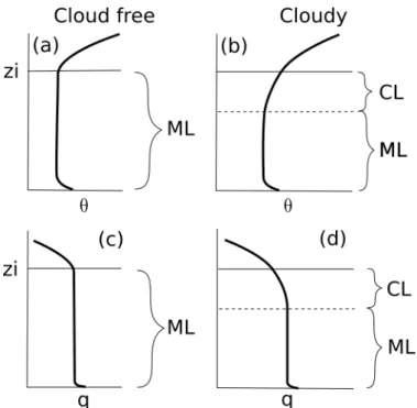
The idealized structure of the boundary layer for potential temperature (θ) and moisture (q) is shown in Figure 2.1. The potential temperature is the absolute temperature, but corrected for adiabatic cooling or heating. Therefore, even if a parcel of air is cooled or heated, its potential temperature stays constant. This is visible in the prole of θ in a cloud free boundary layer (Fig. 2.1a). The area averagedθ is constant with height for the whole boundary layer, up to the inversion or boundary layer height (zi). The convection originating from the surface in the form of sensible and latent heat uxes causes the air to mix, hence the constantθand the name mixed-layer. Also q is in this layer well mixed and constant with height (Fig. 2.1c).

The increase in temperature close to the surface causes a parcel in this region to be less dense than its environment. It therefore has a positive buoyancy. The parcel is in an unstable environment and starts to rise. If the parcel does not experience any phase changes and does not mix with its environment, its temperature changes follow the dry adiabat. That means that the temperature of the parcel is decreasing with height. In the shallow morning boundary layer, the parcel won't condensate and will reach the top of the boundary layer without a phase change. At the top of the boundary layer it reaches the inversion. At the inversion are strong gradients in temperature and moisture. Here the parcel loses its positive buoyancy, but it still has some momentum from the upward motion. This momentum causes it to penetrate the inversion by a bit, thereby mixing some

(16)

2.1 Shallow cumulus formation

Figure 2.1: Idealized proles for a cloud free (a,c) and cloudy (b,d) boundary layer. Shown are the proles for potential temperature (θ) and humidity (q).

Indicated are the boundary layer height (zi), the mixed-layer (ML) and the cloud layer (CL).

air from the free troposphere into the boundary layer. This process is called entrainment and it makes the boundary layer grow over time.

2.1.2 Shallow cumulus formation over land

The growth of the boundary layer results in rising parcels with enough inertia to reach their saturation point. The saturation point of a parcel depends on pressure and temperature, and it makes the water vapour of the parcel condensate. The presence of cloud condensation nuclei (CCN) enhances this process. The height at which condensation happens is called the lifting condensation level (LCL) and it marks the base of the clouds. The phase change of condensation above this height induces heat release and an increase of temperature. The increased temperature gives a parcel positive buoyancy again, causing it to rise further until it reaches the inversion height.

For a boundary layer with clouds the proles of θ and q look slightly dierent than for a boundary layer without clouds (Fig. 2.1b,d). The water vapor condensation above the LCL causes latent heat release, this is visible in the increase ofθ in the cloud layer. Since water vapor condensates, q decreases in this layer. Only a few parcels have enough inertia to reach the LCL and continue to rise and mix air. In the areas without clouds there is no convection and no mixing of air. Therefore a distinction is made between the mixing layer and the cloud layer. Because in both layers turbulence is present, here the combination of the two layers is dened as the boundary layer.

2.1.3 Shallow cumulus formation in the subtropics

Shallow cumulus not only form over land in the mid-latitudes, they also often occur over the ocean in the subtropics. The thermodynamic processes are similar for both locations,

(17)

2.2 Observing shallow cumulus clouds

Figure 2.2: A schematic representation of the Hadley cell (Stevens, 2005)

but in the subtropics the main driver of convection is the typical circulation of air instead of the diurnal cycle of the heating of the surface. The steady large scale circulation is referred to as the Hadley circulation or Hadley cell (Tiedtke et al., 1988). A schematic is given in Figure 2.2. At the equator, ocean temperatures are high and winds converge, this causes the air to rise and creates favourable conditions for the formation of deep convection. Higher aloft the winds diverge north- and southwards, creating large areas of signicant subsidence at higher altitudes. In these areas the dominant type of clouds are stratocumulus. The winds owing back from these subsidence regions towards the equator are called the trade winds. Their name comes from the fact that they are steady and predictable and traders proted from them. These trade winds enhance evaporation of ocean water and trigger moist convection. The boundary layer therefore deepens which causes a decoupling of stratocumulus from the surface. The stratocumulus breaks open, this is called the stratocumulus to cumulus transition. The moist convection as a consequence of the trade winds results in the formation of Cu, in this region also called Trade wind cumulus. ShCu moisten the boundary layer, and this moisture is advected by the trade winds towards the equator where it promotes the formation of deep convection.

2.2 Observing shallow cumulus clouds

Because of their frequent occurrence, impact on the atmosphere and uncertain role in climate change, the study of shallow cumulus clouds is of importance. Observations of ShCu are very useful for this. However, observing cloud populations is not easy because of their complex character and large horizontal spread. Satellite measurements are a type of measurements able to observe entire cloud populations. Several satellite products are freely available, but they dier in resolution and observed locations. For cloud populations, satellite data has been used to study their spatial distribution (Joseph and Cahalan, 1990), also in comparison with model data (Tobin et al., 2012). Another source of observational data comes from point measurements. A good example of a measurement site that specically focuses on clouds is JOYCE (Jülich ObservatorY for Cloud Evolution), located in south-western Germany (Löhnert et al., 2015). The aim of the observatory is to improve the understanding of cloud formation and precipitation processes. Measured are vertical proles of temperature and humidity and cloud properties. One instrument that is currently being developed further is a scanning radar. This instrument has potential in providing 3D data about clouds and observing cloud size distributions in nature (Borque

(18)

2.3 Modelling shallow cumulus clouds

et al., 2014). Further eorts in observing cloud populations include eld campaigns where air planes y through clouds and measure microphysical properties (e.g. Rauber et al.

(2007)).

2.3 Modelling shallow cumulus clouds

Although input from measurements is absolutely necessary for our understanding of cloud processes, they cannot be used for weather and climate predictions and for sensitivity studies. For that numerical models have to be used. As described earlier, the representation of ShCu in said models is an important source of uncertainty. The main reason for this is their scale. ShCu are typically small and live shortly, in contrast to the large spatial and temporal scales on which numerical weather prediction (NWP) and climate models operate.

The large scales are the only ones directly resolved by the model equations. Processes that are smaller than the grid spacing are called subgrid scale and unresolved, their contribution to the mean state is approximated by a parametrization scheme. Each parametrization scheme has its own uncertainties which contribute to the large uncertainty associated with cloud representation in climate models. Disentangling which eect comes from which scheme is dicult, the interaction between the schemes makes that the errors of one scheme might be compensated for by an other (Siebesma2004). An example of an uncertainty is present in the surface scheme. Here the Monin Obukhov Similarity Theory (MOST) is used to determine the surface heat uxes, but the theory is only valid for homogeneous surfaces. In the case of a heterogeneous surface the total eect is approximated. The possible extra eects of surface heterogeneities are disregarded.

2.3.1 Parametrization schemes for shallow cumulus

The subgrid-scale ShCu are represented by a cloud scheme, which strongly interacts with the schemes for boundary layer processes, land surface, microphysics, radiation and convection. The cloud scheme determines the cloud cover from the thermodynamic conditions of the atmosphere, which are given by the convection and boundary layer scheme. It also takes care of the condensation and evaporation processes. The boundary layer scheme is responsible for the turbulent transport of heat, moisture and momentum which depend on the surface conditions given by the land surface scheme. All processes concerning the formation of cloud droplets and precipitation are included in the microphysics. The interaction with aerosols as CCN is present here as well. The radiation scheme determines the available energy in terms of radiation. Lastly, the convection scheme controls the transport of organized thermals.

These organized thermals in the convection scheme are problematic because they cover a large range of scales. They are present in large synoptic scale events, high and low pressure systems, fronts, thunderstorms as well as small individual clouds. Because of the large range of scales, convection is partly resolved and partly parametrized. To parametrize convection many options are available. Some schemes explicitly divide deep and shallow convection, while others opt for a unied approach (Hohenegger and Bretherton, 2011).

Apart from handling the division of scales dierently, other avours are possible as well;

one can e.g. include stochastics (Plant and Craig, 2008) or conditional Markov chains (Dorrestijn et al., 2013).

(19)

2.3 Modelling shallow cumulus clouds

2.3.2 Grey zone of convection

The uncertainty associated with parametrized clouds can in theory be solved by increasing the model resolution. There has been much eort in this direction, supported by the ongoing development of technology and computer systems, making it possible to run atmospheric models on higher resolutions without having to compromise on domain size.

However, the increased resolutions are not quite high enough to resolve all convection. At the same time, the common assumption in convection schemes that a thermal covers only a small part of a grid cell, is not valid any more at high resolutions. The in-between state of not resolving but also not accurately parametrizing convection is termed the grey zone, or Terra Incognita (Wyngaard, 2004). As a reaction to this problem, work is being done on scale-aware and scale-adaptive convection schemes. Depending on the grid resolution, the scale below which convection is parametrized is determined. One example of a scale-aware scheme is the ED(MF)ⁿ scheme (Neggers, 2015). This scheme uses several plumes (up- drafts), each representing a dierent scale. The foundation for a scheme like this has been laid by Arakawa and Schubert (1974), who introduced a cloud size distribution (CSD) based scheme. By using a scheme with a CSD at its foundation, the great variation of cloud sizes can be taken into account and at the same time their scale can be accounted for. For this approach to be successful, information is needed on the dependence of convective processes on cloud size and scale and an accurate description of the cloud population in terms of size is necessary. Studies suggest that the CSD can best be described by a power law with a scale break (Heus and Seifert, 2013). For scales larger than the scale break, the power law is not suitable any more. However, the reason for the scale break and its position are not well understood. Because of the importance of a correct representation of the shape of the CSD for the development of scale-aware convection schemes, the CSD is studied in more detail in Chapter 3 of this thesis.

2.3.3 Large Eddy Simulation

To study ShCu populations and their size distributions, we will not use observations or larger scale models with parametrized clouds, but a Large Eddy Simulation (LES) model.

The advantage of a LES model is that it explicitly resolves the dominant scales of turbulent motion in the boundary layer, meaning neither clouds nor convection are parametrized and only the small subgrid scales are parametrized (Smagorinsky1963, Deardor1970). Because of the high resolutions, it is computationally too expensive to do global simulations with an LES, but the regional scale domains can be large enough to study local cloud processes.

An LES model provides 3D output with a high temporal frequency, which is necessary for studying cloud populations. LES models can be highly idealized in terms of large-scale ow or surface conditions, but they are a valuable tool to study isolated processes or the interaction between specic processes. By initializing LES for dierent regimes, many processes can be studied and the impact of dierent situations can be assessed with the help of sensitivity studies. Results from studies like this are benecial for the formulation of parametrization schemes. In this study two dierent LES models with dierent set-ups are being used: DALES (Dutch Atmosphere Large Eddy Simulation, Heus et al. (2010)) and ICON-LEM (ICOsahydral Nonhydrostatic Large Eddy Model, (Zängl et al., 2014;

Dipankar et al., 2015; Heinze et al., 2017)). The models and their set-ups are described in more detail in the chapters where they are used.

(20)

2.4 Thesis outline

The aim of this thesis is assessing the inuence of surface heterogeneity on spatial patterns in shallow cumulus cloud populations. To this end, research rst focuses on describing shallow cumulus populations in terms of size and spacing. In Chapter 3 we look into the cloud size distribution of shallow cumulus clouds. Given the strong diurnal cycle of ShCu formation over land, we employ many LES simulations for days with ShCu where for each simulation the daily cycle is captured. For the shape of the CSD a power law-exponential function is proposed, instead of a power law with scale break. The power law-exponential function captures the CSD over the complete range of cloud sizes and a scale break does not have to be taken into account.

Chapter 4 focuses on the relation between cloud size and cloud spacing. This relation is shown to be linear (Joseph and Cahalan, 1990). These ndings were based on satellite observations, but nowadays models are available that are able to resolve ShCu over large domains. We employ an ICON simulation over the subtropical Atlantic which features many clouds per snapshot. With this data the dependence of cloud spacing on cloud size is studied. The cloud size dependency is a necessary piece of information for the development of CSD based parametrization schemes (Neggers et al., 2019). The results show that dierent denitions of cloud spacing result in dierent functional relations with cloud size. The spacing between clouds of a similar size is of special interest for scale- adaptive convection schemes, it is found to exponentially depend on cloud size.

In Chapter 5 several parameters to quantify convective organization are compared. The organization parameters are all applied in literature, but they all have their own advantages and disadvantages. For the comparison again the ICON data over the subtropical Atlantic is used, since it has many clouds and some interesting patterns in the cloud eld. Not all compared parameters are able to capture the transition from more organized to less organized cloud elds, something that can be observed by eye from snapshots. Based on the results one parameter that performs best is selected for later use.

The results from previous chapters give the tools and knowledge to tackle the main objective presented in Chapter 6, which is the inuence of surface heterogeneity on the shallow cumulus cloud populations. By using a set of ICON simulations with diering surface conditions, the impact of these surface conditions on the CSD and cloud organization can be assessed. The simulations are centred around JOYCE and dier in topography and land use type distribution. The sensitivity for these boundary conditions on ShCu is assessed for two dierent days. Small dierences for the CSD are found, the slope is not aected by the surface conditions. However, the range of cloud size does change. For enhanced topography the maximum cloud size increases. A clear dierence in organization can not be observed when looking at the organization parameter. Visual inspection and an extra analysis on the variance of vertical wind speed suggests that there might be dierences between the elds that are not being picked up by the organization parameter.

(21)

Chapter 3

Investigating the diurnal evolution of the cloud size distribution of

continental cumulus convection using multi-day LES

This chapter is published as: Thirza W. van Laar, Vera Schemann and Roel A.J. Neggers (2019), Investigating the Diurnal Evolution of the Cloud Size Distribution of Continental Cumulus Convection Using Multiday LES. Journal of the Atmospheric Sciences, vol. 76, no.3, doi: 10.1175/JAS-D-18-0084.1.

Abstract

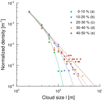
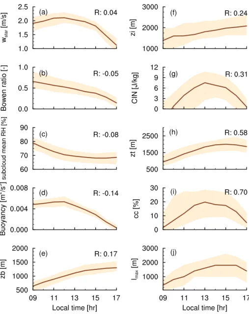
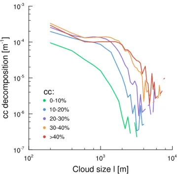
The diurnal dependence of cumulus cloud size distributions over land is investigated by means of an ensemble of large-eddy simulations. 146 days of transient continental shallow cumulus are selected and simulated, reecting a low mid-day maximum of total cloud cover, weak synoptic forcing and the absence of strong surface precipitation. The LES simulations are semi-idealized, forced by large-scale model output but using an interactive surface. This multitude of cases covers a large parameter space of environmental conditions, which is necessary for identifying any diurnal dependen- cies in cloud size distributions. A power law-exponential function is found to describe the shape of the cloud size distributions for these days well, with the exponential component capturing the departure from power law scaling at the larger cloud sizes. To assess what controls the largest cloud size in the distribution, the correlation coecients between the maximum cloud size and various candidate variables reecting the boundary layer state are computed. The strongest correlation is found between total cloud cover and maximum cloud size. Studying the size density of cloud area revealed that larger clouds contribute most to a larger total cloud cover, and not the smaller ones. Besides cloud cover, cloud base and cloud top height are also found to weakly correlate with the maximum cloud size, suggesting that the classic idea of deeper boundary layers accommodating larger convective thermals still holds for shallow cumulus. Sensitivity tests reveal that the results are only minimally aected by the representation of microphysics and the output resolution.

(22)

3.1 Introduction

Shallow cumulus clouds play an important role in Earth's weather and climate system.

Both the mean amplitude and the variability of cloud cover have a signicant impact on the earth's radiation budget (Cahalan et al., 1994). This requires a correct representation of the spatial structure of a shallow cumulus cloud eld in climate and weather prediction models, in order to adequately simulate the radiative uxes.

A complicating factor is that shallow cumulus clouds need to be parametrized because of their small and highly variable temporal and spatial scale. Various recent studies have identied such cumulus parametrizations to be at the heart of problems in both numerical weather prediction and climate simulations (Bony and Dufresne, 2005; Neggers and Siebesma, 2013; Vial et al., 2016). An active area of research which addresses a part of this problem focuses on the feedback of shallow cumulus clouds to climate perturbations (Zhang et al., 2013; Brient et al., 2015; Dal Gesso et al., 2015). Another problem for cumulus parameterization is the increasing resolution of the climate and NWP models and thereby the approach of the grey zone (Wyngaard, 2004). This means that parameterization schemes have to become sensitive for the resolution used in the model and be scale-adaptive. Moreover, it also means that our understanding of the spatial structure and diurnal cycles of cumulus cloud elds has to be improved. This is therefore actively re- searched at the moment (Arakawa and Wu, 2013; Dorrestijn et al., 2013; Kwon and Hong, 2016; Honnert, 2016).

In essence, making a cumulus scheme scale-aware means that size information somehow has to be included. This has recently motivated researchers to revisit the approach of formulating models in terms of cloud size distributions (CSDs), following Arakawa and Schubert (1974). Recent studies with CSD-based schemes by Wagner and Graf (2010), Park (2014), Neggers (2015) and Brast et al. (2018) report promising skill in reproducing scale-adaptivity, however closure of the CSD is still needed. This closure is still an open research question, and needs to be informed by reliable statistics on cloud sizes and their dependence on meteorological conditions.

Cloud size distributions for shallow convection have been investigated by numerous previous studies, using both observational and model data. Some older studies, like Plank (1969) and Wielicki and Welch (1986), report an exponential distribution, whereas later work commonly describes the functional form of the cloud size distribution with a power law:

N(l) =a l^b, (3.1)

withlthe cloud size andaandbtting constants. A power law for cloud size distributions has been applied in observational studies like Benner and Curry (1998) and Zhao and Di Girolamo (2007) as well as LES studies like Neggers et al. (2003) and Heus and Seifert (2013). Jiang et al. (2008) used a power law as well to describe cloud size properties and they showed a good comparison between observations and model data. Recently, Feingold et al. (2017) used a power law distribution for their study on the relation between albedo and cloud cover. The power law exponent b from Eq. (3.1) describes the slope of the distribution. Typical values that have been found are between -1.7 and -2.5 (Rieck et al., 2014).

Many observational and modelling studies report the existence of a scale break in the power law (recently e.g. Trivej and Stevens (2010); Heus and Seifert (2013)), meaning that the pure power law t is only valid for the small cloud sizes. For clouds larger than the scale

(23)

3.1 Introduction

break the slope of the power law needs to be adjusted to t the data, resulting in a double power law. How to determine the location of this scale break in a methodical way, as well as the underlying cause for this break in scaling, are still actively debated in the literature.

Benner and Curry (1998) mention a break in fractal dimension at a location similar to the scale break in their CSD for which the underlying reason could be a maximum size of individual convective cells (Joseph and Cahalan, 1990), while Wood and Field (2011) hypothesise that the Rossby radius controls the characteristic cloud sizes and thereby the scale break. A third possible cause for the scale break is insucient statistics; the sampling size is too small to capture the full distribution, in particular at the largest sizes which occur least frequently. Also domain size and resolution might inuence the location of the scale break in a simulated cloud eld.

Since it is hard to estimate the position of the scale break in a standardized way and its background is unclear, we follow Windmiller (2017) and Peters et al. (2009) in their approach of applying a power law-exponential function to the CSD. The power law- exponential t is exible to capture many shapes, from a pure power law to a more curved t. By applying this t we avoid having to explicitly deal with the scale break. The power law-exponential function is based on percolation theory and is dened as (Ding et al., 2014):

N(l) =a l^b exp(c l), (3.2)

withc representing another tting constant. Both theband c are expected to be smaller than or equal to 0 and together they reect the shape of the distribution. With decreasingc the distribution follows less a power law and is increasingly dominated by the exponential, especially at the large cloud sizes.

While the shape is one dening aspect of the CSD, its range in terms of size is another. An early study by Joseph and Cahalan (1990) suggests that the maximum cloud size scales with the depth of the boundary layer. More recently, Rieck et al. (2014) conrmed this dependence, but also reported that surface heterogeneity plays a role. Dawe and Austin (2012) found a strong relationship between the cloud area and the eventual height reached by the cloud. Sakradzija and Hohenegger (2017) showed that the shape of the distribution of cloud-base mass ux, which is closely related to the cloud size distribution, is determined by the Bowen ratio at the surface. While these new insights are encouraging, many of these studies were limited to single cases, or even single snapshots. Such snapshots do not contain any information on the diurnal evolution of the maximum cumulus cloud size. In addition, the use of single cases limits the statistical signicance of the obtained results. To assess the robustness of the results and to obtain information on the diurnal signal of the maximum cloud size one would need a database of many dierent cases covering a broad parameter space of large-scale conditions.

For this study, a library with 146 individual cumulus days is created to investigate the behaviour of the size distribution during diurnal cycles of cumulus over land. Continental shallow cumulus cases are chosen because of their transient nature, with a strong temporal evolution in the amount of clouds, their elevation and depth, and the size distribution.

Using many dierent days over the course of 5 years enables us to do statistical studies on cloud size controlling factors on a diurnal time-scale. For all the selected days a 24- hour Large-Eddy Simulation (LES) simulation is performed, and a clustering algorithm is applied to compute the cloud size distribution and study both its shape and the maximum cloud size. Correlations between the maximum cloud size and a set of candidate variables are calculated to establish the role of these variables in controlling the upper limit of the distribution of cloud sizes. Sensitivity tests are performed with a subset of cases on the output resolution and the microphysics representation.

(24)

3.2 Multi-day LES

The conguration of the LES experiments and the case selection is described in section 2. In section 3 the clustering algorithm and the derivation of the cloud size statistics is explained, followed by the results in section 4 and 5. Finally, discussion and conclusions can be found in sections 6 and 7.

3.2 Multi-day LES

The derivation of statistically signicant size distributions requires 3D cloud elds that contain a sucient number of clouds and are available at a frequency high enough to resolve any diurnal signal. While the latest scanning radar strategies show promising capability in detecting CSDs in nature (Borque et al., 2014), this technique is still in its infancy and needs to be fully explored. We therefore still rely on LES simulations to complement observational data with 3D elds at high frequencies (Neggers et al., 2012;

Schalkwijk et al., 2015; Zhang et al., 2017). For this study daily LES as applied at the meterological supersite JOYCE (Jülich ObservatorY for Cloud Evolution) in Germany will be used.

3.2.1 JOYCE

The observational supersite JOYCE (Löhnert et al., 2015) is a continental mid-latitude site, well suited to study diurnal cycles. It is equipped with state of the art cloud detec- tion instrumentation which are operational on the long-term. Mid-latitude cumulus are regularly present at JOYCE during summer, since the site is close enough to the sea to ensure that low-level humidity is frequently high enough to allow daytime cumulus formation. The abundance of long-term observations allows for confronting LES with relevant observational data, this is however not the focus of this study and is considered a future research topic. The measurements taken at JOYCE will only be used for the selection of shallow cumulus days and a short comparison of the measured and modelled cloud cover.

3.2.2 Cumulus day selection

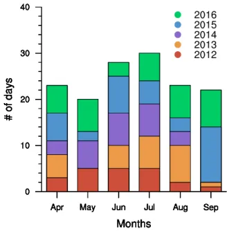
Since the focus of this research is on boundary layer cumulus clouds, days which show this cloud regime have been selected to be simulated. Several specic criteria are applied to visualized reectivity of lidar and radar observations taken at JOYCE. Selected days do not show any precipitation and no signicant synoptic scale activity during daytime. They do have a signicant period of cumulus convection around noon and an increase of the LCL during the day. Cloud covers are small and the cumulus events are isolated, which means that they are not inuenced by synoptic events at the beginning and ending of the day. These criteria are applied on the summer months of the years 2012-2016, in the winter months conditions are usually too cold for shallow cumulus to form. The result is a selection of 146 days in total. How these days are distributed over the years and the months can be seen in Figure 3.1. The resulting library of cases provides us with a parameter space of considerable width. By simulating all 146 days individually, and not simulating a single composite like Zhang et al. (2017), the internal variability of the ensemble is resolved.

This provides additional information on the robustness of any diurnal signal in the CSD properties, as well as its spread for the environmental conditions covered by the library of cases. Since we are interested in the diurnal cycle, only the daytime hours between 9 and 17 hr are used for further analysis.

(25)

3.2 Multi-day LES

Figure 3.1: Histogram showing how the total of 146 days are spread over the months and years.

3.2.3 DALES

The Dutch Atmospheric Large-Eddy Simulation (DALES, Heus et al. (2010)) model is used for the simulation of the selected days. DALES has taken part in many recent intercomparison studies on shallow cumulus convection (e.g. van Zanten et al. (2011);

van der Dussen et al. (2013)) which document its skill in simulating this cloud regime.

The land surface parametrization scheme is described in Heus et al. (2010) and it is similar to the ECMWF surface scheme. In the simulations, the state of the land surface is evolving with time-varying temperature and soil moisture. As a result, the surface energy uxes are also time-varying, calculated interactively through the surface energy budget. For the calculation of the vertical transfer of radiative energy Monte Carlo Spectral Integration is used, as described in detail by Heus et al. (2010). The resolved turbulent domain reaches up to 5 km. Above this height, the vertical prole of the thermodynamic and cloudy state of the IFS analysis is used to calculate the downward transfer of radiative energy into the turbulent domain, by which the impact of clouds overhead are accounted for.

In addition, a climatological vertical prole of ozone is provided to the radiation scheme.

The domain size of the simulations is 12.8x12.8x5 km, with a resolution of 50 m in the horizontal and 40 m in the vertical direction. Simulations start at 00:00 LT (LT leads UTC by two hours in European Summer in Germany) and cover one full day (24 hours). Every 15 minutes, every 4th point of the three-dimensional eld of all required model variables is saved for further analysis. This sub-sampling is done in order to keep the amount of data manageable. The impact of the reduced data output on the CSD will be assessed (as reported in the Appendix, section 3.8), showing only marginal dependence, which supports taking this approach. Zhang et al. (2017) report a dependence of the total cloud cover on the featured micro-physics scheme. In the simulations the two-moment parameterization scheme of Seifert and Beheng (2004) is used, but its dependence on the results is tested.

A sensitivity study is performed by using some additional simulations with a simple non- precipitating all-or-nothing cloud scheme by Sommeria (1976) that are done for the years 2013 and 2014.

(26)

3.2 Multi-day LES

3.2.4 Initialization, boundary conditions and large-scale forcing

The 24-hour long simulations are initialized and driven by time-varying boundary conditions and large-scale forcings derived from the Integrated Forecasting System (IFS) of the European Centre for Medium-range Weather Forecasts (ECMWF). The method as applied here to drive the LES model was rst described by Neggers et al. (2012), and was recently used in slightly modied form in the study by Gesso and Neggers (2018). All elds provided to the LES as input are based on two analysis elds per day, at 00:00 and 12:00 UTC, supplemented by short-range forecast elds to cover the intermediate timepoints at 3, 6 and 9 hours. This eectively yields a forcing dataset covering 24 hours at 3 hour time-resolution, which is assumed sucient to resolve diurnal and synoptic signals in the large-scale forcing.

The initialization of the height-dependent atmospheric state variables concerns the wind componentsuandv, the liquid water potential temperatureθ_l, total water specic humidity q_t, the cloud state variables liquid and ice condensateq_landq_i, and ozone (for the radiation scheme). Also initialized are the soil temperature and moisture, the latter scaled to preserve the fraction between the eld capacity and wilting point (Neggers et al., 2012). After initialization, all these variables are allowed to evolve freely, apart from ozone which is not changing with time.

The prescribed boundary conditions at the surface include the surface geopotential, the albedo, the roughness lengths for heat and momentum, the leaf area index (LAI), and the near-surface air pressure. For both the LAI and the roughness lengths the IFS values at this location are extracted from the MARS archive (ECMWF, 2017). Only the near-surface air pressure changes with time, determining the geometric height of the pressure levels in the prole above. The soil temperature and moisture can evolve freely but interact with the atmosphere, through the surface energy and humidity budgets. In this respect the LES experiments in this study dier from those in other recent LES studies at supersites, which typically use a fully prescribed soil state (Heinze et al., 2016; Gustafson et al., 2017).

The impact of large-scale weather systems, which can be signicant at mid-latitude locations, is represented by means of prescribed advective forcing tendencies in the budget equations of the four atmospheric state variables{q_t, θl, u, v}. This forcing is both height- and time-dependent, and is also continuous, being interpolated linearly between the 3- hourly IFS time-points. IFS data at pressure levels is used to this purpose, in order to avoid problems with advective calculations in areas of steep orography that arise when terrain- following coordinates are used (Simmons and Burridge, 1981; Simmons, 1986). Orography is not included in the simulation, justied by the fact that the direct vicinity of the site is relatively at. The horizontal tendencies are calculated from the wind components and the local gradients on the 0.1x0.1 degree operational IFS grid, averaged over a 0.5x0.5 degree horizontal area around the site of interest to obtain smoothly varying forcing elds. The vertical component of large-scale advection is calculated interactively from a prescribed subsidence prole that acts on the vertical gradients in the model state variables. Momen- tum is forced using a prescribed large-scale horizontal pressure gradient, appearing in the resolved Navier-Stokes equations as a prescribed geostrophic wind, and by accounting for the Coriolis force. The momentum equations take the form as discussed in any standard academic textbook on atmospheric dynamics, for example Holton and Hakim (2012).

Finally, following Neggers et al. (2012) the proles of{q_t, θ_l, u, v}are continuously nudged to the IFS-derived state at a synoptic time-scale of 6 hours. Relaxation at this synoptic time-scale has been proven tight enough to eectively limit excessive model drift, but still loose enough to allow the turbulence to act freely.

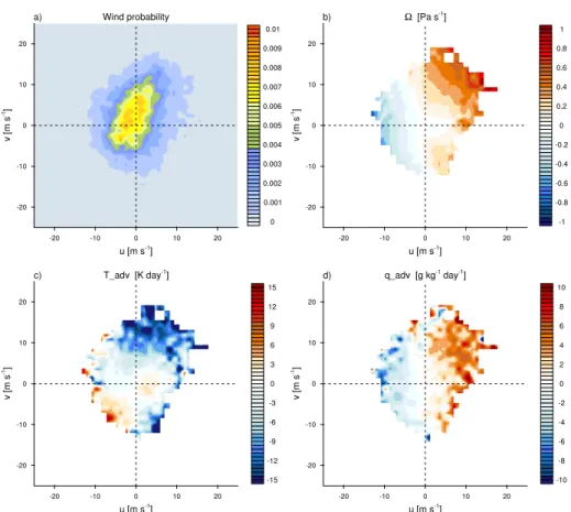
Figure 3.2 gives some insight into the typical summertime large-scale forcing at the JOYCE