Development of Novel Time-Domain Electromagnetic Methods for Offshore

Development of Novel Time-Domain Electromagnetic Methods for Offshore

Groundwater Studies: A Data Application from Bat Yam, Israel

Inaugural-Dissertation

zur Erlangung des Doktorgrades

der Mathematisch-Naturwissenschaftlichen Fakult¨ at der Universit¨ at zu K¨ oln

vorgelegt von Amir Haroon

aus N¨ urnberg

K¨ oln 2016

Gutachter: Prof. Dr. B. Tezkan Prof. Dr. A. Junge

Tag der m¨ undlichen Pr¨ ufung: 07.12.2016

Abstract

Recent marine long-offset transient electromagnetic (LOTEM) measurements yielded the offshore delineation of a fresh groundwater body beneath the seafloor in the re- gion of Bat Yam, Israel. The LOTEM application was effective in detecting this freshwater body underneath the Mediterranean Sea and allowed an estimation of its seaward extent. However, the measured data set was insufficient to understand the hydrogeological configuration and mechanism controlling the occurrence of this fresh groundwater discovery. Especially the lateral geometry of the freshwater boundary, important for the hydrogeological modelling, could not be resolved. Without such an understanding, a rational management of this unexploited groundwater reservoir is not possible.

Two new high-resolution marine time-domain electromagnetic methods are theo- retically developed to derive the hydrogeological structure of the western aquifer boundary. The first is called Circular Electric Dipole (CED). It is the land-based analogous of the Vertical Electric Dipole (VED), which is commonly applied to de- tect resistive structures in the subsurface. Although the CED shows exceptional detectability characteristics in the step-off signal towards the sub-seafloor freshwa- ter body, an actual application was not carried out in the extent of this study. It was found that the method suffers from an insufficient signal strength to adequately delineate the resistive aquifer under realistic noise conditions. Moreover, modelling studies demonstrated that severe signal distortions are caused by the slightest geo- metrical inaccuracies. As a result, a successful application of CED in Israel proved to be rather doubtful.

A second method called Differential Electric Dipole (DED) is developed as an alter- native to the intended CED method. Compared to the conventional marine time- domain electromagnetic system that commonly applies a horizontal electric dipole transmitter, the DED is composed of two horizontal electric dipoles in an in-line configuration that share a common central electrode. Theoretically, DED has sim- ilar detectability/resolution characteristics compared to the conventional LOTEM system. However, the superior lateral resolution towards multi-dimensional resis- tivity structures make an application desirable. Furthermore, the method is less susceptible towards geometrical errors making an application in Israel feasible.

In the extent of this thesis, the novel marine DED method is substantiated using sev- eral one-dimensional (1D) and multi-dimensional (2D/3D) modelling studies. The main emphasis lies on the application in Israel. Preliminary resistivity models are derived from the previous marine LOTEM measurement and tested for a DED ap-

i

ii

plication. The DED method is effective in locating the two-dimensional resistivity structure at the western aquifer boundary. Moreover, a prediction regarding the hydrogeological boundary conditions are feasible, provided a brackish water zone exists at the head of the interface.

A seafloor-based DED transmitter/receiver system is designed and built at the In- stitute of Geophysics and Meteorology at the University of Cologne. The first DED measurements were carried out in Israel in April 2016. The acquired data set is the first of its kind. The measured data is processed and subsequently interpreted us- ing 1D inversion. The intended aim of interpreting both step-on and step-off signals failed, due to the insufficient data quality of the latter. Yet, the 1D inversion models of the DED step-on signals clearly detect the freshwater body for receivers located close to the Israeli coast. Additionally, a lateral resistivity contrast is observable in the 1D inversion models that allow to constrain the seaward extent of this freshwater body.

A large-scale 2D modelling study followed the 1D interpretation. In total, 425 600

forward calculations are conducted to find a sub-seafloor resistivity distribution that

adequately explains the measured data. The results indicate that the western aquifer

boundary is located at 3600 m - 3700 m before the coast. Moreover, a brackish water

zone of 3 Ωm to 5 Ωm with a lateral extent of less than 300 m is likely located at

the head of the freshwater aquifer. Based on these results, it is predicted that the

sub-seafloor freshwater body is indeed open to the sea and may be vulnerable to

seawater intrusion.

Zusammenfassung

Eine vorangegangene marine Long-Offset Transient-Elektromagnetische (LOTEM) Messung in der Gegend von Bat Yam, Israel, verdeutlichte die Abgrenzung eines Grundwasserk¨ orpers unter dem Meeresboden. Die LOTEM-Anwendung konnte diesen Grundwasserk¨ orper unter dem Mittelmeer detektieren und die Ausdehnung eingrenzen. Der gemessene Datensatz ist jedoch nicht ausreichend, um die hydro- geologische Konfiguration und den Mechanismus nachzuvollziehen, die f¨ ur das Auf- treten dieses Grundwasserreservoirs verantwortlich sind. Vor allem die laterale Ge- ometrie der Aquiferkante, die f¨ ur die hydrogeologischen Modellierung relevant ist, konnte nicht aufgel¨ ost werden. Ohne dieses Verst¨ andnis ist eine Bewirtschaftung des ungenutzten Grundwasserreservoirs nicht m¨ oglich.

Zwei neue hochaufl¨ osende marine zeitbereichs-elektromagnetische Methoden sind theoretisch entwickelt worden, um die hydrogeologische Struktur der westlichen Aquiferkante abzuleiten. Die erste Methode ist der Circular Electric Dipole (CED).

Diese Sendekonfiguration ist das Analog-Verfahren zum Vertical Electric Dipole (VED). Dieser wird h¨ aufig zum Detektieren schlechtleitender Strukturen im Un- tergrund angewandt. Obwohl der CED im Ausschaltsignal eine hohe Detektier- barkeit zeigt, um den submarinen Grundwasserk¨ orper zu erkunden, wurde eine praktische Anwendung in der Studie nicht durchgef¨ uhrt. Es wurde festgestellt, dass das CED-Verfahren unter einer unzureichenden Signalst¨ arke leidet, die das Detektieren des Grundwasserleiters unter realistischen Rauschbedingungen nicht erm¨ oglicht. Dar¨ uber hinaus zeigen theoretische Modellierungen, dass starke Sig- nalverzerrungen durch die geringste geometrische Ungenauigkeit verursacht werden.

Daher erschien eine erfolgreiche Anwendung von CED in Israel nicht erfolgsver- sprechend.

Ein zweites Verfahren namens Differential Electric Dipole (DED) wurde als Alterna- tive zu der CED-Methode entwickelt. Im Vergleich zu dem herk¨ ommlichen LOTEM- System, das einen horizontalen elektrischen Dipol-Sender verwendet, besteht der DED-Sender aus zwei horizontalen elektrischen Dipolen in einer Inline-Konfiguration.

Theoretisch weist der DED zu dem herk¨ ommlichen System vergleichbare Detek- tierbarkeit und Aufl¨ osungseigenschaften gegen¨ uber 1D Leitf¨ ahigkeitsstrukturen auf.

Die h¨ oheren lateralen Aufl¨ osungseigenschaften f¨ ur mehrdimensionale Widerstands- strukturen machen eine Anwendung jedoch erstrebenswert. Dar¨ uber hinaus ist das Verfahren f¨ ur geometrische Fehler weniger anf¨ allig als das CED-Verfahren, was eine praktische Anwendung in Israel m¨ oglich macht.

Im Umfang dieser Arbeit wird das neue DED-Verfahren mit mehreren eindimension-

iii

iv

alen und mehrdimensionalen Modellierungsstudien untersucht. Der Schwerpunkt liegt auf der Anwendung in Israel. Vorl¨ aufige Widerstandsmodelle sind aus der fr¨ uheren LOTEM Messung abgeleitet worden und werden f¨ ur eine DED-Anwendung getestet. Das DED-Verfahren lokalisiert die zweidimensionale Widerstand-Struktur auf der westlichen Aquiferkante. Außerdem ist eine Vorhersage ¨ uber die hydrogeol- ogischen Randbedingungen m¨ oglich, sofern sich eine Brackwasserzone an der Spitze der Aquiferkante befindet.

Erste DED-Messungen wurden in Israel im April 2016 durchgef¨ uhrt. Der erfasste Datensatz ist der erste seiner Art. Die gemessenen Daten wurden prozessiert und mittels 1D Inversion interpretiert. Das angestrebte Interpretations-Ziel konnte auf- grund der unzureichenden Datenqualit¨ at der Ausschaltsignale nicht durchgef¨ uhrt werden. Dennoch konnten 1D Inversions-Modelle der Einschaltsignale eindeutig den Grundwasserk¨ orper detektieren. Außerdem ist ein lateraler Widerstandskontrast in den 1D Inversions-Modellen zu beobachten, der auf eine seew¨ artige Abgrenzung dieses Grundwasserk¨ orper hinweist.

Die 1D Inversions-Modelle wurden als Grundlage f¨ ur eine großangelegte 2D Model-

lierungsstudie verwendet. Insgesamt wurden 425 600 Vorw¨ artsrechnungen durchge-

f¨ uhrt, um ein zweidimensionales Widerstandsmodell herzuleiten, dass die gemesse-

nen Daten ad¨ aquat erkl¨ art. Die Ergebnisse zeigen, dass sich die westliche Aquifer-

Kante 3600 m bis 3700 m vor der K¨ uste befindet. Dar¨ uber hinaus ist eine Brack-

wasserzone von 3 Ωm bis 5 Ωm mit einer lateralen Ausdehnung von weniger als 300 m

an der Spitze des Grundwasser-Aquifers wahrscheinlich. Mit diesen Ergebnissen

kann vorhergesagt werden, dass der Grundwasserk¨ orper zum Meer hin wom¨ oglich

offen, und somit f¨ ur das Eindrigen von Meerwasser anf¨ allig ist.

Contents

List of Figures xi

List of Tables xvii

1 Introduction 1

2 State of Research & Motivation 5

2.1 The Coastal Aquifer of Israel . . . . 5

2.1.1 EM Surveys in Israel . . . . 7

2.1.2 Hydrogeological Modelling Studies . . . . 9

2.2 Marine EM Applications . . . 10

2.3 Motivation of the Presented Thesis . . . 11

3 Theory of the Applied EM Methods 13 3.1 Time-Domain Electromagnetic Methods . . . 14

3.1.1 Circular Electrical Dipole . . . 17

3.1.2 Differential Electrical Dipole . . . 18

3.2 Quasi-static Maxwell’s Equations . . . 20

3.3 The Layered Full-Space Model . . . 22

3.3.1 TE and TM Mode . . . 22

3.3.2 1D Forward Operator: Ideal CED . . . 24

3.3.3 1D Forward Operator: Approximated CED and DED . . . 27

3.3.4 Fast Hankel Transformation . . . 29

3.3.5 Code Verification . . . 30

3.4 System Response . . . 31

4 1D-Inversion Theory 33 4.1 General Terms of 1D-Inversion . . . 33

vii

viii CONTENTS

4.2 Non-Linear Inverse Problems . . . 34

4.2.1 Data and Model Parameter Transformation . . . 35

4.2.2 Data Fit . . . 36

4.3 Marquardt Inversion . . . 37

4.3.1 Eigenvalue Analysis . . . 39

4.3.2 Importances . . . 40

4.3.3 Equivalent Models using Monte-Carlo . . . 41

4.4 Occam Inversion . . . 41

4.5 Calibration Factor . . . 43

5 1D Modelling Studies 45 5.1 Background EM Noise Model . . . 46

5.2 Layered Aquifer . . . 47

5.2.1 Detectability of the Aquifer . . . 48

5.2.2 Influence of the Sea-Air Interface . . . 58

5.2.3 Parameter Resolution of the Aquifer . . . 61

5.2.4 Conclusions: Layered Aquifer . . . 65

5.3 Geometrical Errors . . . 66

5.3.1 Non-Verticality . . . 67

5.3.2 Internal Transmitter Symmetry . . . 70

5.3.3 1D Inversion of Geometrically Distorted Data . . . 74

5.4 Summary of 1D Modelling . . . 76

6 2D/3D Modelling of Resistive Formations 79 6.1 3D Forward Operator . . . 80

6.1.1 Grid Design . . . 83

6.1.2 Convergence of the Solution . . . 86

6.2 The 2D Aquifer Model . . . 89

6.2.1 Constructing the Bathymetry Model . . . 90

6.2.2 The Aquifer Boundary . . . 96

6.2.3 1D Inversion of synthetic 2D data . . . 102

6.2.4 Conclusions: 2D Aquifer Model . . . 103

6.3 Signal-Variations of resistive 3D Targets . . . 105

6.4 Summary of 2D/3D Modelling . . . 108

CONTENTS ix

7 Field Survey & Data Processing 111

7.1 Field Survey . . . 111

7.1.1 The DED System . . . 112

7.1.2 Measurement Procedure . . . 113

7.1.3 Field Setup . . . 114

7.1.4 Issues during Data Acquisition . . . 116

7.2 Data Processing . . . 116

7.2.1 Digital Filtering . . . 119

7.2.2 Cutting & Levelling . . . 122

7.2.3 Cluster Analysis . . . 122

7.2.4 Log-Gating and Gate-Stacking . . . 124

7.3 Background Noise Measurements . . . 127

7.4 Field Data . . . 129

7.5 Summary of the Field Survey and Data Processing . . . 131

8 1D Inversion of Field Data 133 8.1 Evaluation of the Current Signals . . . 134

8.1.1 Comparison of Current Signals . . . 134

8.1.2 Significance of the resistive Aquifer . . . 140

8.1.3 Summary of Current Signal Comparison . . . 142

8.2 1D Inversion of all Stations . . . 142

8.2.1 Importances and Resolution Analysis . . . 145

8.2.2 Validating the Results . . . 147

8.3 Calibration Factor . . . 148

8.4 Summary of 1D Inversion . . . 150

9 2D Modelling of Measured Data 153 9.1 2D Interpretation Procedure . . . 155

9.2 Best Fit Models . . . 156

9.2.1 Aquifer Depth, Resistivity and Boundary Position . . . 156

9.2.2 Boundary Shape . . . 166

9.2.3 Summary of 2D Modelling . . . 168

10 Summary & Conclusion 171

x CONTENTS

Bibliography 175

A Setup and Nomenclature 185

B 1D Inversion - Extended 187

C 2D Modelling of Field Data - Extended 193

D Electric Fields of CED and DED 195

E Acknowledgements 199

List of Figures

2.1 Map of the coastal aquifer of Israel. . . . 6

2.2 Cross section of the coastal aquifer in Israel. . . . 7

2.3 Results of TDEM measurements along the coastal plain of Israel. . . 8

2.4 1D Occam inversion results from LOTEM. . . . 9

2.5 Hydrogeological modelling study from the Palmahim disturbance. . . 10

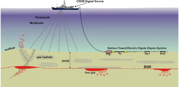
3.1 Marine TD-CSEM setup . . . 14

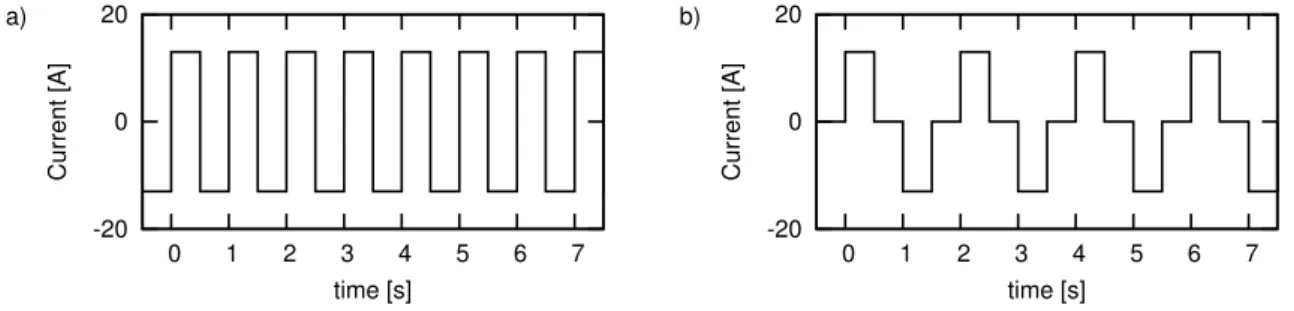
3.2 Square wave current signals. . . 15

3.3 Step-on and step-off electrical fields. . . 16

3.4 Sketch of the real and the ideal CED . . . 17

3.5 Schematic of a seafloor-based DED system . . . 19

3.6 Layered earth model consisting of N layers below the source and M layers above . . . 23

3.7 Illustration of the current density j and magnetic flux density b for TE mode on the left and TM mode on the right (Weidelt , 1986). . . . 24

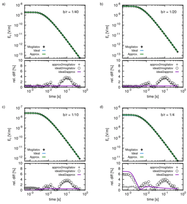
3.8 CED transients calculated with three different algorithms at an offset of 200 m from the CED centre . . . 31

5.1 Exemplary transients and associated noise models for marine LOTEM measurements in Israel . . . 47

5.2 Layered aquifer model applied for 1D modelling studies . . . 48

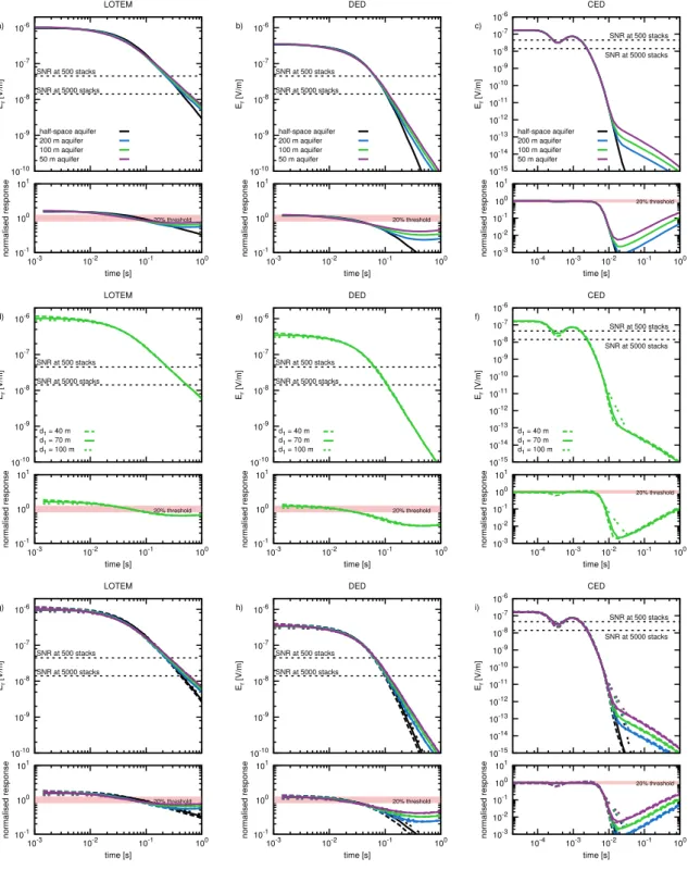
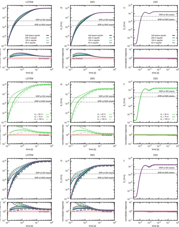
5.3 Step-off transient for a layered aquifer model in the shallow sea envi- ronment . . . 50

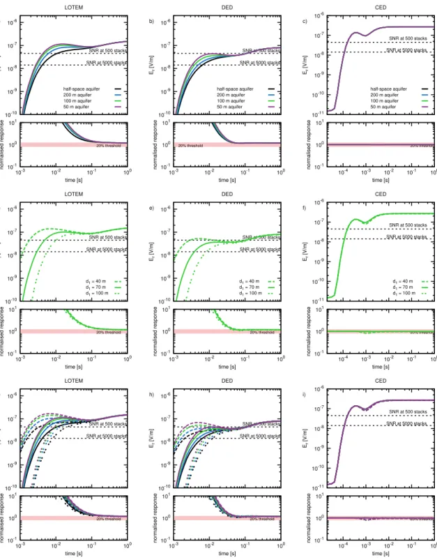
5.4 Step-on transient for a layered aquifer model in the shallow sea envi- ronment . . . 52

5.5 Layered earth model in a deep ocean of 3000 m. . . 54

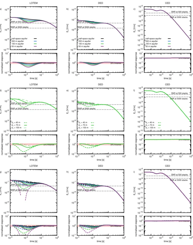
5.6 Step-off transient for a layered aquifer model in the deep sea environ- ment . . . 55

xi

xii LIST OF FIGURES 5.7 Step-on transient for a layered aquifer model in the deep sea environ-

ment . . . 56

5.8 1D resistivity models used to investigate the influence of the airwave . 59 5.9 Impulse response of different resistivity models to study the airwave. . 60

5.10 Synthetic data calculated for a shallow marine model. . . 62

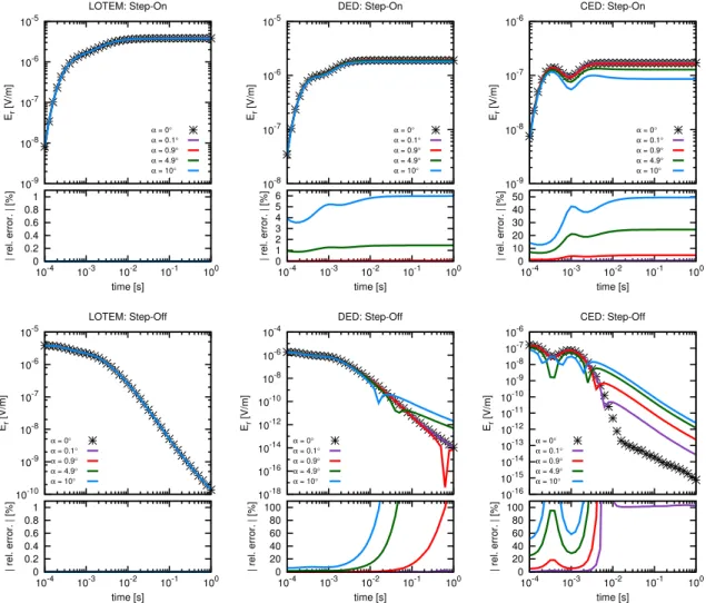
5.11 Eigenparameter analysis for synthetic LOTEM, DED and CED data . 63 5.12 Schematic of non-verticality configuration for VED, CED and DED transmitters . . . 68

5.13 Non-verticality effect of VED (a and d), CED (b and e) and DED (c and f) . . . 69

5.14 Relative errors displayed as a function of tilt-angle and time for a VED source . . . 70

5.15 Geometrical error study investigating dipole movements of (a) LOTEM, (b) DED, and (c) CED . . . 70

5.16 Transients and relative errors investigating geometrical errors and displayed for LOTEM, CED and DED . . . 72

5.17 RMS errors displayed as a function of geometrical error . . . 73

5.18 1D Occam inversion model for distorted step-off data . . . 74

5.19 1D Occam inversion model for distorted step-on data . . . 75

6.1 Example of a Yee-grid cell . . . 81

6.2 Geometry for averaging conductivities with current flow in x-direction 82 6.3 Finite difference grid of a CED transmitter. . . . 84

6.4 Finite difference grid of a DED transmitter . . . 85

6.5 Grid checks for CED and DED transmitters using one-dimensional resistivity models . . . 87

6.6 Output parameters (a) RES, (b) PROGN and (c) EPS . . . 88

6.7 Sketches of the true, approximated 2D and 1D bathymetry models . . 90

6.8 Synthetic transients of a 2D bathymetry model . . . 91

6.9 Study of 2D bathymetry model using 1D forward modelling . . . 93

6.10 1D Marquardt inversion of different 2D bathymetry models . . . 95

6.11 Schematic sketches of the 2D resistivity model used for modelling. In (a) the aquifer is blocked to the sea and no seawater encroachment occurs. In (b), seawater intrusion is occurring without a mixed-water zone ahead. In (c), a brackish water zone is located ahead of the freshwater body. . . 97

6.12 DED profile plots for three different aquifer models . . . 98

LIST OF FIGURES xiii 6.13 DED transients at selected stations for the tree different aquifer models 99 6.14 DED profile plots for the Intrusion and Blockage model aquifer ex-

cluding the bathymetry . . . 101

6.15 1D Occam R1 inversion models of synthetic 2D data. . . 103

6.16 3D modelling study representing a hydrocarbon saturated formation . 106 6.17 Profile plots of CSEM, VED, DED and CED for a hydrocarbon re- sistivity model . . . 107

7.1 Sketch of the applied DED-transmitter/receiver system . . . 112

7.2 Impressions during the field survey . . . 114

7.3 Map of the survey area near the coastline of Bat Yam, Israel . . . 115

7.4 In-line DED electric field data measured during the test measure- ments in Cuxhaven, Germany. The power spectra of the recorded time series is displayed in (a). All recorded channels are displayed in (b) and the shifted time-series is displayed in (c). . . 117

7.5 (a) Power spectra and (b) time series segment of electrical field data measured at station p16NR. In blue, the raw data is displayed, in orange the filtered data. . . 120

7.6 (a) Power spectras and (b) time series segments of electrical field data measured at station p11FR. The data was filtered multiple times using the three-point filter starting from period lengths of 18 s (orange) and incrementally decreasing to period lengths of 2 s (light blue). This approach is used to minimise the long-periodic noise. . . 121

7.7 Cluster analysis of measured DED data . . . 123

7.8 Normal probability plots at a selected intermediate time of t = 0.2512 s124 7.9 Exemplary illustration of how data is log-gated using the data ac- quired at station p16NR . . . 125

7.10 Comparison between log-gated/gate-stacked data and smoothed data 127 7.11 Background EM noise measurements from station p12NR . . . 128

7.12 Processed transients at station p03FR . . . 129

7.13 Processed transient of Rx1 (FR) and Rx2 (NR) plotted against the position along the profile . . . 130

7.14 Profile plots of the data measured at the far receiver for selected time points. . . 131

8.1 Inversion models obtained from the step-on transient at station p03FR135 8.2 Inversion models obtained from the step-off transient at station p03FR136 8.3 Models obtained from the joint inversion at station p03FR . . . 137

8.4 Graphical SVD-analysis of the weighted Jacobian . . . 138

xiv LIST OF FIGURES 8.5 Modelling studies investigating the significance of the resistive aquifer

layer . . . 141

8.6 Occam Inversion models for Step-On signals of roughness 1 (top) and 2 (bottom) plotted against the receiver positions along the profile . . 143

8.7 Marquardt inversion models for Step-On signals plotted against the receiver positions along the profile . . . 144

8.8 Data fit of inversion models at selected stations . . . 144

8.9 SVD analysis for selected Marquardt inversion models . . . 145

8.10 Modelling studies investigating the significance of the resistive aquifer layer . . . 147

8.11 Occam R2 and Marquardt inversion models obtained for free (red lines) and fixed (black lines) calibration factors at stations p04FR, p08FR and p16NR displayed in a, b and c, respectively . . . 149

9.1 The 2D model consisting of five model parameters . . . 153

9.2 Scatter plots of the model parameters ρ ₁ , ρ ₂ , d ₁ and d ₂ vs. the χ. . . 157

9.3 Distribution of model parameter combinations for the 2D model ac- quired for transients of Zone A . . . 158

9.4 Measured and calculated transients for all equivalent models obtained in Zone A . . . 159

9.5 Accumulation of models with χ ≤ 1 to identify the most likely bound- ary position . . . 160

9.6 Scatter plots of the model parameters ρ ₁ , ρ ₂ , d ₁ and d ₂ vs. the χ for equivalent models obtained in Zone B. . . . 161

9.7 Data fit of profile plots for selected delay-times of 3.2 ms and 8.0 ms . 162 9.8 Equivalence domain in dependency of three model paramters for x a = 3600 m and x _a = 3700 m . . . 164

9.9 Measured and calculated transients for all equivalent models obtained in Zone B . . . 165

9.10 The 2D model consisting of five model parameters . . . 166

9.11 Data fits of data from Zone B for possible western aquifer boundary conditions. . . 167

9.12 Final 2D resistivity model for offshore Bat Yam, Israel . . . 169

B.1 SVD analysis for several stations along the profile. . . 187

B.2 SVD analysis for several stations along the profile. . . 188

B.3 Inversion models of step-on signals for stations p01FR through p09FR

in (a) through (h), respectively. . . 189

LIST OF FIGURES xv B.4 Inversion models of step-on signals for stations p10FR through p17NR

in (a) through (h), respectively. . . 190

B.5 Joint-Inversion models of step-on/off signals for stations p01FR through p09FR in (a) through (h), respectively. . . 191

B.6 Joint-Inversion models of step-on/off signals for stations p10FR through p17NR in (a) through (h), respectively. . . 192

C.1 χ-errors for all equivalent models along the profile . . . 193

C.2 Distribution of CF values at each station in Zone B . . . 193

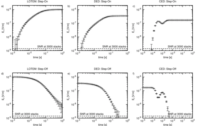
D.1 Total electric field for CED step-on at selected times . . . 195

D.2 Total electric field for CED step-off at selected times . . . 196

D.3 Total electric field for DED step-on at selected times . . . 197

D.4 Total electric field for DED step-off at selected times . . . 198

List of Tables

6.1 True water depths for the three exemplary transmitter positions. . . . 94 8.1 Importances of model parameters from the Marquardt inversion: 0 -

0.5 poorly resolved (-). 0.51 - 0.7 (o) moderately resolved. 0.71 - 1.0:

well resolved (+). The CF is kept fixed at 1 for all inversion models. . 139 8.2 Importances of model parameters from the Marquardt inversion: 0 -

0.5 poorly resolved (-). 0.51 - 0.7 (o) moderately resolved. 0.71 - 1.0:

well resolved (+). . . 146 9.1 Model parameters tested in the 2D modelling study to fit the mea-

sured DED data. For the stations of Zone B, all combinations of five parameters are tested. Stations of Zone A are only tested for the resistivity and thickness parameters. . . . 155 9.2 Model parameter variation for the 2D modelling study to fit the mea-

sured data. . . . 169 A.1 Information to receiver positions from the measurements. . . 185

xvii

Chapter 1

Introduction

Electromagnetic (EM) induction methods are commonly applied to determine the resistivity distribution within the subsurface. In principle, these methods can dis- tinguish a target formation from its surroundings if a resistivity contrast exists. In terms of studying the salinity of groundwater aquifers in coastal regions, EM meth- ods are particularly effective, as the pore-fluid salinity has a direct influence on the electrical resistivity. The resistivity of water decreases with increasing salinity. In Israel, Goldman et al. (1988) quantifies the resistivity of seawater saturated sedi- ments to be between 0.5 Ωm and 1.5 Ωm. Freshwater saturated sediments will have resistivity values of greater 10 Ωm (Kafri and Goldman , 2006).

An onshore time-domain EM (TDEM) application along the coastal plain of Israel investigated the resistivity values of the lower coastal sub-aquifers (Kafri and Gold- man, 2006). Direct borehole salinity/conductivity measurements confirmed that regions of increased resistivity are linked to aquifer systems occupied with fresh to brackish water, whereas areas of low resistivity contained mainly saline water. The largest region of interest is a 20 km long transect known as the Palmahim Distur- bance, located between the cities of Ashdod in the South and Bat Yam in the North.

Marine Long Offset Transient Electromagnetic (LOTEM) measurements conducted by the Institute of Geophysics and Meteorology (IGM) at the University of Cologne, confirmed the offshore extent of this freshwater body to approximately 3.5 km from the coastline (Lippert et al., 2012; Lippert , 2015). However, the measurements could not explain why this region of the lower coastal sub-aquifer contains fresh ground- water. The insufficient lateral resolution of the applied LOTEM method, in addition to the sparse data density around the western aquifer boundary prohibited an ade- quate assessment of the transition zone between the freshwater aquifer and seawater saturated sediments.

A further attempt to answer this question was granted in January 2014 by the German Research Foundation (DFG) in a project called: “Marine Circular Electric Dipole (MCED): An innovative electromagnetic method used for the exploration of groundwater resources”. The presented thesis is conducted in the framework of this three-year project. The initial consideration of the project intended the ap- plication of a method called marine Circular Electric Dipole (CED). Mogilatov and Balashov (1996) introduced this method for land-based EM applications as an al- ternative to the Vertical Electrical Dipole (VED) to avoid the necessity of using boreholes. Their applied CED transmitter antenna consists of eight horizontal elec- tric dipoles (HEDs) arranged in a star-shaped pattern around a common central

1

2 CHAPTER 1. INTRODUCTION electrode. The excited EM field for a surface-based CED is analogous to that of a VED. The land-based application utilises a transmitter with several hundred metres radii in addition to mobile magnetic field receivers to map three-dimensional resis- tivity structures (Helwig et al., 2010a,b). The intended marine application aimed at decreasing the transmitter radius to approximately 10 m, while using electric field receivers at short-offsets of approximately 50 m. The advantage of such application is the enhanced lateral resolution compared to the marine LOTEM method (Ha- roon et al., 2013). Theoretically, the acquired step-off signal can clearly distinguish between different hydrogeological structures at the sub-seafloor freshwater aquifer boundary. However, the intention of applying the MCED had to be abandoned in August 2014, due to the insights gained during theoretical modelling studies. These proved that the complex structure of the CED transmitter is extremely susceptible towards geometrical inaccuracies. Even small deviations of several millimetres cause pronounced distortions in the received signal. These modelling studies are found in Haroon et al. (2016) and are presented and elaborately discussed in the extent of this thesis.

To minimise the distortions caused by these geometrical errors, it was decided to simplify, and elongate the CED transmitter. The result is a completely new trans- mitter antenna consisting of two HEDs in an in-line configuration that share a common central electrode. This novel EM method is called Differential Electrical Dipole (DED). Compared to the standard in-line LOTEM application, DED has an enhanced lateral resolution, especially in the short-offset configuration (Haroon et al., 2016).

In the framework of this thesis, extensive theoretical modelling studies are conducted investigating the advantages and disadvantages of CED and DED compared to the conventional LOTEM and VED methods. An excerpt of these studies is published in Haroon et al. (2016) for a hydrocarbon application. The main focus of this thesis lies on studying the signal characteristics for the expected groundwater model in Israel, including detectability, resolution and signal distortion caused by geometrical inaccuracy. Moreover, the lateral resolution characteristics of DED are investigated using a 2D resistivity model. As an application of CED proved to be impractical, the 2D modelling studies focus mainly on the application of DED. However, an excerpt of the lateral resolution capabilities of CED is found in Goldman et al. (2015) and Haroon et al. (2016).

One interesting aspect that evolved in the extent of the theoretical modelling studies is the noticeable difference between step-on and step-off transients for seafloor-based EM systems within shallow marine settings. It appears that the received signals of either current excitation are sensitive towards different model parameters, provided the seawater layer above the transmitter/receiver system is shallow. This effect is independent of the current excitation and also applies for LOTEM signals. The differences of both signal types are emphasised in all modelling studies conducted in the context of this thesis.

The first marine DED measurements were conducted in April 2016 with the partners

at EcoOcean, who were responsible for all technical issues concerning the research

vessel “Mediterranean Explorer”. During the four-day measurement, 22 receiver sta-

3 tions were acquired along the profile of Lippert (2015). Issues arose at five receiver stations, which are therefore not considered in the interpretation. The acquired data is processed and interpreted using newly developed processing and 1D inver- sion software ¹ . It is shown using synthetic data, that the acquired step-on signal retrieves a realistic sub-seafloor resistivity structure if certain conditions regarding the bathymetry are respected. The 1D inversion of the measured data will therefore indicate if the DED method can detect the resistive sub-seafloor aquifer.

Subsequently, a multi-dimensional interpretation of the measured DED data is sought. A multi-dimensional time-domain inversion software for marine DED is presently not available. Recently, Yogeshwar (2014) applied 2D inversion on mea- sured in-loop TDEM data based on the code of Martin (2009). However, this al- gorithm is designed for surface-based sources and has not been applied for marine LOTEM or DED data sets. Therefore, a large-scale 2D modelling study is realised to fit the measured DED step-on data. The main objectives yield the delineation of the aquifer boundary, including shape and hydrogeological structure. In total, over 425 600 forward calculations are carried out on the HP-Cluster at the University of Cologne. An ensemble of resistivity models that best describes the measured data set is found and evaluated.

Finally, the results are summarised and evaluated in connection to the first marine DED application. An outlook for necessary developments is given to improve the acquisition and interpretation process in the future.

Thesis Overview

The presented thesis has the following structure. First, the scientific background of groundwater studies in Israel and marine EM applications is presented. This overview includes previous EM applications in the region (Kafri and Goldman , 2005, 2006; Lippert , 2015) and groundwater flow studies (Amir et al., 2013). Furthermore, the standard marine EM application is introduced. The development of a new ap- plication technique is motivated based on the limitations of the existing EM systems within shallow water. Finally, the objectives of this thesis are motivated and classi- fied on the basis of the current state of research. In Chapter 3 and Chapter 4, the basic theory of the applied EM methods and inversion techniques are introduced. In Chapter 5, a one-dimensional earth model is assumed and several modelling studies are realised. Detectability, resolution and geometrical errors of the novel meth- ods are investigated and compared to the conventional marine EM systems. The 2D submarine aquifer model of Lippert (2015) is incorporated into the theoretical assessment of the DED method in Chapter 6. The multi-dimensional forward mod- elling is performed with sldmem3t from Druskin and Knizhnerman (1994). Chapter 7 through 9 deal with the DED application in Israel and the subsequent data analy- sis. In Chapter 10, a conclusion of the presented work is given along with an outlook of necessary future DED developments.

1 Technically, only the forward solutions for CED and DED are newly developed. These are

implemented in the existing 1D inversion software MARTIN of C. Scholl.

4 CHAPTER 1. INTRODUCTION Preliminary Notes

The presented work will stick to the following convention. Unless stated other- wise, all presented electric fields are source current normalised. Although they are displayed in V/m, the correct dimensions should actually read V/Am. To avoid confusion, I renounce from this terminology. Furthermore, all vectors are written in bold lower-case letters, whereas matrices are displayed in bold upper-case letters.

This also applies to the vector quantities in the EM theory.

The modelling studies presented in this thesis are largely based on the resistivity

models derived by Lippert (2015). I therefore recommend reading his work prior to

this one.

Chapter 2

State of Research & Motivation

The following chapter will give an overview of the scientific background to motivate the developments made in the context of this thesis. First, the groundwater situa- tion in Israel is presented emphasising the coastal aquifer and the phenomenon of the sub-seafloor freshwater body around the Palmahim Disturbance. Several studies have been published regarding the coastal aquifer of Israel. The first section of this chapter constrains to the previous work of Kafri and Goldman (2005, 2006) and Lippert (2015). A brief review of the geophysical groundwater studies performed by the IGM Cologne in Israel is given. Groundwater flow simulations conducted by Amir et al. (2013) are introduced for two possible aquifer scenarios in the Palmahim region. The first assumes an aquifer that is open to seawater intrusion, the second a closed aquifer scenario. The derived subsurface salinity distribution of Amir et al.

(2013) motivates an EM application to delineate the hydrogeological structure of the seawater/freshwater interface. The conventional marine EM methods are intro- duced, focussing mainly on the limitations in shallow sea environments. Based on these limitations, the development of novel time-domain EM methods is justified, as they will help to distinguish between the two aquifer scenarios. Taking the presented scientific background into account, the main objectives of this thesis are explained.

2.1 The Coastal Aquifer of Israel

Groundwater reservoirs in coastal regions are particularly vulnerable to contamina- tion due to the continuing natural threat of seawater rise. Anthropogenic influences, caused by the increased urbanisation, also lead to a deterioration in groundwater quality. In Israel, this situation is pronounced as population steadily increases, while the coastal regions of the Mediterranean Sea are already densely populated. Fur- thermore, the coastal aquifer is one of only three national water system reservoirs (Kafri and Goldman , 2006). The salinity content of this aquifer has increased in the last decades due to over exploitation, anthropogenic pollution and artificial recharge (Amir et al., 2013; Kafri and Goldman, 2006).

Displayed in Fig. 2.1 is the southern and central coastal aquifer of Israel that ex- tends from Hadera in the North to the Gaza Strip in the South. It is replen- ished by the mountainous aquifer and drains into the Mediterranean Sea. The lateral extent of the aquifer from the Mediterranean Sea to the foothills is between 8 km in the North, and 30 km in the South with a thickness of 200 m or less

5

6 CHAPTER 2. STATE OF RESEARCH & MOTIVATION

Figure 2.1: Map of the coastal aquifer in Israel (grey area) showing the Palmahim area. The cross section A - A’ is studied in a 2D hydrogeological groundwater flow simulation presented in Section 2.1.2, investigating which hydrogeological condi- tion enables the existence of fresh groundwater in the lower sub-aquifers (Amir et al., 2013).

(Amir et al., 2013). The aquif- erous units consist mainly of sand and calcareous sandstone that are separated by aquiclu- dal clay formations near the coast, which thin out towards the East. As displayed in Fig. 2.2, the aquifer is gen- erally divided into four sub- aquifers named A, B, C and D from top to bottom. The up- per sub-aquifers A and B, are phreatic. Due to the saline wa- ter detected in these depth in- tervals, the basic assumption is that sub-aquifers A and B are prone to seawater encroach- ment throughout the entire Is- raeli coastal plain. Kapuler and Bear (1970) assume that this also applies to the lower sub-aquifers. However, Kolton (1988) challenges their assump- tion, stating that the lower sub- aquifers (C and D) thin out to- wards the Mediterranean Sea in the West and pass into a continuous shale sequence that blocks the lower sub-aquifers from seawater intrusion. His theory is based on the Nordan 4 Wildcat borehole located be- tween Ashqelon and Gaza (see Fig. 2.1), which shows a thick continuous shale sequence be-

low the upper sub-aquifers (Kafri and Goldman, 2006). Kafri and Goldman (2006) summarise observations that support the described possibilities of Kolton (1988) and Kapuler and Bear (1970). For instance, the water age obtained from the lower sub-aquifers is older than that of the upper ones, indicating restricted interaction.

This may suggest that the lower aquifers are confined, whereas the upper aquifers

are prone to seawater intrusion. Yet, the lower sub-aquifers are intruded by salt wa-

ter in many areas along the coastal plain of Israel, suggesting that all sub-aquifers

are open to the sea.

2.1. THE COASTAL AQUIFER OF ISRAEL 7

Figure 2.2: Typical cross section of the coastal aquifer in Israel (Kafri and Gold- man, 2005). Near the coastline, the coastal aquifer is divided into four separate sub-aquifers named A through D. The intermediate clay formations thin out to- wards the land. The lower aquifer is bounded by the Saqiye clay formation.

2.1.1 EM Surveys in Israel

TDEM methods are useful for groundwater studies due to the relationship between pore-water salinity and the corresponding electrical resistivity. Saltwater saturated sediments found in the coastal regions are less resistive compared to the same sed- iments saturated with fresh water. Therefore, areas of increased resistivity values within the depth range of the lower sub-aquifers indicate the presence of brackish or fresh water. First groundwater TDEM experiments in Israel are presented by Gold- man et al. (1988), studying the freshwater/seawater interface in northern Israel.

These measurements are followed by Nuclear Magnetic Resonance (NMR) mea- surements for groundwater exploration (Goldman et al., 1994). The IGM Cologne actively started investigating the groundwater situation in Israel by applying the LOTEM method in northern Israel (Scholl , 2005). Later, Kafri and Goldman (2006) published work on the coastal aquifer south of Tel Aviv, which motivated a further IGM study in Israel (Lippert, 2015) and the presented thesis.

Kafri and Goldman (2006) conducted several TDEM measurements along the coastal plain of Israel, investigating the resistivity (salinity) of the lower coastal sub-aquifers.

An excerpt of their study is presented in Fig. 2.3. The authors correlated their find- ings to borehole data, which found regions within the central and southern coastal aquifer that are occupied with fresh water. The largest region is a 20 km long strip located south of Tel Aviv and north of Ashdod, generally referred to as the Palmahim Disturbance. These fresh water findings are related to the assumption that the lower sub-aquifers are locally blocked to the sea.

The IGM Cologne started a joint project with the Israel Oceanographic and

8 CHAPTER 2. STATE OF RESEARCH & MOTIVATION

Figure 2.3: Map of southern Israel including TDEM stations investigating the resistivity in the depth range of the lower sub-aquifers C and D (Kafri and Goldman, 2006).

Limnological Research (IOLR) and the Geophysical Institute of Israel (GII) that was funded by the German Federal Min- istry of Education and Research (BMBF) and the Israeli Min- istry of Science, Technology and Space (MOST) between 2008 and 2011 to explore the westward extent of the lower sub-aquifers in the Palmahim area underneath the Mediter- ranean Sea. In the extent of this project, marine LOTEM measurements were conducted along a transect running per- pendicular to the coastline off the shore of Bat Yam, Israel.

The full interpretation of the acquired data set is found in Lippert (2015). The following is an excerpt of his main find- ings to motivate the applica- tions conducted in the extent of this thesis.

Displayed in Fig. 2.4 are 1D Occam inversion models ob- tained from marine LOTEM data. Clearly, the marine LOTEM measurements were ef-

fective in detecting the sub-seafloor aquifer off the coastline of Bat Yam, Israel

(Lippert , 2015). Furthermore, the application was also effective in restraining the

lateral extent of the sub-seafloor aquifer, predicting the western boundary to be

located between 3.25 − 3.65 km from the coastline. The results enabled preliminary

hydrogeological modelling based partly on still unknown assumptions (Amir et al.,

2013). This includes the location and nature of the western aquifer boundary that

could not yet be assessed due to the insufficient lateral resolution of the LOTEM

method. Lippert (2015) applies synthetic modelling studies to show that marine

LOTEM is capable of differentiating between the hydrogeological structures at the

aquifer boundary, provided a sufficient data density, and knowledge about the exact

boundary position is available. However, the exact position of the boundary was not

known prior to the LOTEM campaigns and is still vague within a range of about 400

m. An EM data set with a sufficient station density is needed, preferably using a

method with high lateral resolution, to further constrain the boundary position and

gain information regarding the hydrogeological structure of the aquifer transition

zone.

2.1. THE COASTAL AQUIFER OF ISRAEL 9

Figure 2.4: 1D Occam inversion results obtained from marine LOTEM measure- ments (modified after Lippert (2015)). A resistive layer interpreted as the sub- seafloor freshwater body extends to approximately 3.25−3.65 km from the coastline.

2.1.2 Hydrogeological Modelling Studies

Hydrogeological modelling studies were performed in the extent of the BMBF-MOST project by Amir et al. (2013). The following is only an excerpt of the hydrogeological simulation. As displayed in Fig. 2.5, the authors differentiated between two possible aquifer scenarios. The first scenario, displayed in the top images of Fig. 2.5, assumes an aquifer system where the lower sub-aquifers are open to the sea. The second scenario assumes an aquifer system that is closed to the sea by a sharp boundary located 9 km before the coast. Note, Amir et al. (2013) did not take the LOTEM results of Lippert (2015) into account, else the aquifer boundary would be located closer to the shoreline.

The simulations show the steady state condition for a hydraulic conductivity of K = 0.001 m/day in the separating layers. The necessary conditions for a freshwater occurrence at the shoreline are investigated. For the selected hydraulic conductivity, both aquifer scenarios satisfy this occurrence. However, a gradual salinity gradient is pronounced for the open aquifer scenario, whereas the closed aquifer scenario is characterised by a sharp salinity transition reproducing the shape of the initial model. In this case a vertical boundary. The differences in the salinity variations may produce a measurable EM signature, provided the lateral resolution of the applied EM method is sufficiently high.

Based on these hydrogeological flow simulations, three possible resistivity models

are derived for the 2D modelling studies. These are displayed in Fig. 6.11 and will

be explained in detail in the corresponding section. Basically, the first two models

exemplify either a closed aquifer scenario with a vertical boundary or a partially

closed scenario with a typical wedge-shaped boundary. The third model exemplifies

the open aquifer scenario with a zone of decreased salinity (resistivity) at the head

of the saltwater/freshwater interface. If an apparent DED response is measurable

between the three models is extensively studied in Chapter 6.

10 CHAPTER 2. STATE OF RESEARCH & MOTIVATION

a) b)

d) c)

km

km

Figure 2.5: Hydrogeological modelling study for a schematic cross section of the coastal aquifer in the Palmahim region. The left column displays the cross section A - A’ from Fig. 2.1 for (a) an open-aquifer scenario and (c) a closed-aquifer scenario.

The four subdomains are 1) the upper aquifers A and B, 2) the lower aquifers C and D, 3) the undivided coastal aquifer and 4) the separating clay layers. The images on the right display the modelling results for a hydraulic conductivity of K

= 0.001 m/day for (b) an open-aquifer scenario and (d) a closed-aquifer scenario.

The colours correspond to the salinity of the contained water, which is related to the resistivity value. Images are modified after Amir et al. (2013).

2.2 Marine EM Applications

The idea of using electromagnetic (EM) methods to study sub-seafloor resistivity structures dates back to Cagniard (1953). He proposed using the Magnetotelluric (MT) method as a tool to study the resistivity structure beneath the seafloor. Since then, numerous publications proposed the application of a horizontal electrical dipole transmitter with a continuous, low frequency wave excitation along with seafloor based receivers to map the sub-seafloor resistivity structure, e.g. Filloux (1967); Cox et al. (1986); Constable and Cox (1996). This method became generally known as the frequency-domain controlled source electromagnetic (FD-CSEM or just CSEM) method. The main advantage of CSEM is the exceptional detectability towards resistive layers. Consequently, the method has become quite popular in hydrocarbon prospecting ever since Ellingsrud et al. (2002) first applied CSEM on an offshore oil field. A review of the CSEM method is found in Constable (2010).

CSEM experiments are generally difficult to conduct in shallow-sea environments

due to the saturation of the acquired signal at large offsets, known as the airwave

effect (Chen and Alumbaugh, 2011). As a consequence, CSEM loses its sensitivity

towards the resistive layers in the subsurface. Different strategies have been devel-

oped to account for the effect of the airwave. For example, Chen and Alumbaugh

(2011) present three strategies to mitigate the effect of the airwave: (1) EM buck-

ing, (2) dE/dFreq and (3) MT impedance stripping. However, these approaches are

often inaccurate due to simplified assumptions and are sometimes controversial.

2.3. MOTIVATION OF THE PRESENTED THESIS 11 CSEM applications in the time-domain, generally referred to as TD-CSEM or marine LOTEM (only in Cologne) are also applied frequently, e.g. Schwalenberg et al.

(2010); Hunziker et al. (2011); H¨ olz et al. (2015); Lippert (2015). The advantage of an application in the time-domain is that the airwave can be separated in the early time data (Ziolkowski and Wright, 2007). A detailed analysis between TD- signals and FD-signals for shallow water experiments is given by Weiss (2007). He shows that the signature of the target formation in the subsurface is not necessarily masked by the signature of the airwave in the TD-signal. Further applications use a VED transmitter, which excites an EM field that is independent of the airwave (Haland et al., 2012; Singer and Atramonova , 2013; Helwig et al., 2013). Note, the airwave is only present in five of six electromagnetic field components using a HED source (Weidelt , 2007) and remains absent in the vertical electrical field. Due to reciprocity, this also applies to VED transmitters.

Recently, first applications using VED sources have been published (Holten et al., 2009; Helwig et al., 2013). These applications constrain to measuring vertical elec- tric fields at the receiver, as they are less prone to errors caused by non-verticality.

This effect is investigated by Goldman et al. (2015), who show that VED measure- ments require perfectly vertical transmitters/receivers to avoid parasitic effects from contributing to the acquired signal. Even small deviations may result in strong dis- tortions in the acquired signal. Furthermore, the application of VED in shallow water is problematic due to the limited extent of the vertical source. Unless very large current amplitudes are applied, the acquired signal will generally exhibit a poor signal-to-noise ratio (SNR). For applications in Israel, a VED source is not feasible due to the limited extent of the water column (< 40 m).

2.3 Motivation of the Presented Thesis

The presented work is completed in the framework of the DFG project (GZ:TE 170/19-1) “Marine Circular Electric Dipole (MCED): An innovative electromagnetic method used for the exploration of groundwater resources”. The original goals of the project include the development of a new MCED system. An application of MCED in Israel shall clarify if the lower sub-aquifers (C and D) are indeed open or closed to seawater intrusion. During the theoretical developments prior to the first intended measurement, modelling studies proved that an application is not feasible in the extent of the project due to various technical issues. These will be elaborately explained in Chapter 5 of this thesis. As a result, an alternative method called Differential Electric Dipole (DED) is developed to resolve the hydrogeological structure of the sub-seafloor aquifer.

A seafloor-towed transmitter and receiver system is built at the Institute of Geo-

physics and Meteorology, Cologne, Germany. Compared to the previous marine

LOTEM measurements, where the offset between transmitter and receiver was not

stringently known, a fixed-offset system is developed to minimise the geometrical

errors and increase the accuracy of the measurement. Additionally, new transmitter

(ZT30: Zonge International) and receiver (KMS-820: KMS Technologies) devices

are implemented into system. The latter required the development of a new time-

12 CHAPTER 2. STATE OF RESEARCH & MOTIVATION series processing software. The processing steps are explained and illustrated in Chapter 7. Test measurements were conducted in Cuxhaven - Sahlenburg (January 2016) to test the system and the developed software, but are not addressed in the framework of this thesis.

The content of the presented work deals with the practical and theoretical develop- ment of the marine CED and DED methods. This includes the development of a 1D forward algorithm for both methods, which is implemented in the existing 1D inver- sion software “Marine TEM Inversion Program - MARTIN” of C. Scholl. Theoretical studies are realised using 1D modelling and 3D modelling with sldmem3t of Druskin and Knizhnerman (1994). For the latter, a new finite-difference grid generator is developed to accompany the discretisation of the CED transmitter. Ultimately, only DED is applied during the measurements in Israel due to the complexity and geometrical issues concerning the CED.

The first marine DED measurement was conducted in April 2016 with the following aims:

1. Feasibility study of the new marine DED system.

2. Validating the results previously obtained by marine LOTEM. Is a resistive layer detectable in the vicinity of the coastline using marine DED?

3. Locate the position of the western aquifer boundary more accurately compared to the marine LOTEM measurements.

4. Investigate the hydrogeological structure at the aquifer boundary to draw con- clusions about the possible seawater intrusion scenarios.

The acquired data is processed and interpreted using the developed software. Subse- quently, a large-scale 2D modelling study is conducted to fit the measured data using the 1D inversion results as a basis. The parameter space is systematically investi- gated between minimum and maximum values for each model parameter. The final 2D results are presented as an ensemble of models that best describe the measured data set.

The projected goal of this work is to present a fully functional marine DED system

that is applicable in the shallow marine environment. Furthermore, software devel-

opments shall allow an interpretation of the measured data with the ultimate goal

of applying marine DED in other coastal regions in the future.

Chapter 3

Theory of the Applied EM Methods

The basic theory of TDEM methods is based on the electromagnetic diffusion equa- tion in conductive media. The electrical conductivity or its inverse, the electrical resistivity are the essential physical material property to which the applied TDEM methods are sensitive. The propagation of electric current through the earth is gen- erally classified into three mechanisms: electrolytic, electronic and dielectric con- duction (Telford et al., 1976). In the coastal regions of Israel, mainly sedimentary rocks are found. The current propagation is therefore dictated by electrolytic (ionic) conduction, where the resistivity of the porous rock varies with the mobility and con- centration of the dissolved ions. The controlling factors are the state of the pores, and the amount and conductivity of the contained fluid. Resistive fluids like hydro- carbons or fresh water increase the sediment resistivity and can be targeted using TDEM methods (Gehrmann , 2014). In comparison, sedimentary rocks saturated with salt water will have much lower resistivity values (Darnet et al., 2010). Con- sequently, TDEM methods are not only effective in hydrocarbon exploration, e.g.

Ellingsrud et al. (2002), but are also commonly applied for groundwater studies in coastal regions, e.g. Kafri and Goldman (2006).

The empirical formula of Archie (Archie, 1942) relates the resistivity of a fully saturated host medium ρ ₀ to the resistivity of the contained pore fluid ρ _w with

ρ 0 = aφ ^−m ρ w , (3.1)

for clean sands. This relationship was developed for clay-free sands only, but is commonly used to analyse marine sediments that contain fair amounts of clay. In Eq. (3.1), φ is the porosity and a is a coefficient introduced by Winsauer et al.

(1952) that is theoretically equal to one, but practically not equal to one. m is a further empirical Archie parameter (Spangenberg , 2001). Small values of a and m describe sediments with well-interconnected pore spaces, as ρ ₀ then decreases. If we assume that a, φ and m remain constant for a specific rock formation and degree of saturation, and solely the resistivity of the pore fluid ρ _w dictates the value of ρ ₀ , then TDEM methods can determine if the porous rock formation contains fresh water or salt water.

In the following, marine TDEM applications are introduced both practically and theoretically. The main emphasis lies on the novel CED and DED methods studied

13

14 CHAPTER 3. THEORY OF THE APPLIED EM METHODS in the extent of this thesis. The general concepts of EM applications are found in Ward and Hohmann (1988). The specific theory of a HED source in a layered marine environment is found in Edwards (1997). The CED method is presented by Mogilatov (1992), Mogilatov and Balashov (1996) and Haroon et al. (2016). The theory to VED and loop sources in a layered marine environment are found in Scholl and Edwards (2007) and Swidinsky et al. (2012), respectively.

The basic principles and source current excitations of TDEM methods are intro- duced. Subsequently, Maxwell’s quasi-static equations are used to derive the basic diffusion equation. A simplified one-dimensional (1D) earth model, consisting of stratified layers of homogeneous conductivity is introduced and the forward solu- tion of a CED and DED source located on any layer boundary is derived. The forward operator is described regarding its implementation in the 1D inversion soft- ware MARTIN. The implementation is verified using comparative modelling studies with existing software (Mogilatov and Zlobinsky , 2008). Finally, the system response is addressed.

3.1 Time-Domain Electromagnetic Methods

In the following, the basic principles of TD-CSEM in the marine environment are described. The general description is extended to the specific EM sources developed in the context of this thesis.

As illustrated in Fig. 3.1, a seafloor-based marine TD-CSEM system generally con- sists of a HED transmitter along with several electric field receivers at fixed offsets in an in-line configuration. The injected source current is often a square-wave signal

Figure 3.1: Schematic setup of a typical TD-CSEM measurement applied in the

marine environment. The system consists of a HED transmitter accompanied by

electrical field receivers in an in-line configuration (Schwalenberg et al., 2010).

3.1. TIME-DOMAIN ELECTROMAGNETIC METHODS 15

-20 0 20

0 1 2 3 4 5 6 7

Current [A]

time [s]

-20 0 20

0 1 2 3 4 5 6 7

Current [A]

time [s]

a) b)

Figure 3.2: Square wave current signals for (a) 100% and (b) 50% duty cycle with current amplitudes of 13 A and a period of 1 s and 2 s, respectively.

with either 100% duty cycle displayed in Fig. 3.2a, or a 50% duty cycle displayed in Fig. 3.2b. The term duty cycle refers to the percentage in which the transmitter is in an active state. At each station, the ship will stop and measure for several minutes to ensure decent data quality (Schwalenberg et al., 2010). The system positioning is commonly maintained using acoustic transponders in the leading weight (PIG).

As mentioned, two types of current signals are often applied. These are displayed in Fig. 3.2. For a 100% duty cycle signal, the transmitter switches the polarity directly without an intermediate pause. These polarity switches are generally interpreted as step-on signals with a twofold current amplitude. In this case, it is assumed that the transmitter is inactive at t < 0 s and is switched on at t = 0 s. In contrast, the 50% duty cycle signal has intermediate phases between polarity switches, where no current is transmitted. Accordingly, both step-on and step-off transients are obtained when applying a 50% duty cycle. A step-off transient is constant at t < 0 s and decays after the transmitter is turned off at t = 0 s. The relationship between step-on f ^On and step-off f ^{Of f} signals is expressed as

f ^{Of f} = f ^DC − f ^On , (3.2)

where f ^DC describes the signal at the direct current (DC) level.

Marine TD-CSEM applications generally apply a 100% duty cycle signal due to the increased SNR. The resulting signals are interpreted as a step-on transients, e.g. Schwalenberg and Engels (2011). An interpretation of step-off signals is only feasible when applying a 50% duty cycle. This approach is commonly applied for in- loop TEM measurements (Asten, 1987) due to two particular technicalities. First, the step-off function of modern transmitter systems is generally quicker and cleaner compared to the step-on function (Lippert, 2015). Second, the DC plateau is not completely constant, but actually oscillates around a particular value. These oscil- lations may appear in form of noise at the receiver. In this case a step-off signal is more robust, as no primary EM field superimposes the measured signal. Par- ticularly magnetic field measurements benefit from the characteristics of a step-off current signal. Appropriately, Lippert (2015) interpreted step-off signals in a marine LOTEM experiment, where magnetic fields were also measured.

Exemplary step-on and step-off transients are illustrated in Fig. 3.3 by blue and

red lines, respectively. The DC level is displayed by a dashed black line. The time

16 CHAPTER 3. THEORY OF THE APPLIED EM METHODS

10 ^-9 10 ^-8 10 ^-7 10 ^-6

10 ^-3 10 ^-2 10 ^-1 10 ⁰

E x [V/m]

Time [s]

Step on Step off DC-Level

Figure 3.3: Exemplary electric field for a step-on (blue) and step-off (red) current excitation. The DC level is displayed by a black dashed line. The quasi-DC ranges of the respective transients are displayed by blue and red background colours.

range in which the corresponding signal is in the quasi-DC range is marked by the respective background colours. In general, the step-on signal is characterised by an increase of signal amplitude that is dependent on the subsurface resistivity structure.

A more resistive subsurface will result in a steeper increase of the acquired signal.

Alternatively, the step-off signal begins at the DC level and decays proportionally to the subsurface resistivity structure. A more resistive subsurface will cause a steeper decay of the signal amplitude.

One issue that is brought into conjunction with step-off signals is the poor SNR at late times. Unfortunately, the response of the respective target formation often appears at these late times. Therefore, the step-on signal is usually applied in marine TD-CSEM measurements, as SNR is a common issue, especially if deep resistive targets are investigated. The studies presented in this thesis will demonstrate that the signals of step-on and step-off for shallow sea EM applications are sensitive towards different model parameters. This phenomenon has not been thoroughly investigated in literature and is evaluated using 1D/2D resistivity models in the extent of this thesis.

In recent years, marine TD-CSEM applications did not confine to the application of HED sources. Goldman et al. (2015) states that the relative target response towards an intermediate resistive layer, embedded in a conductive background, is increased if a VED source is applied. The authors base their arguments on the two separate modes of the EM field within a 1D background environment. Commonly theses are referred to as the transverse electric (TE) mode and transverse magnetic (TM) mode.

A detailed description of the TE and TM mode is found in Chapter 3.3.1 of this

thesis. Any EM application using a HED transmitter with horizontal electric field

receivers is considered bimodal, since both modes are excited. Unimodal applications

either use a VED source for a pure TM field or Vertical Magnetic Dipoles (VMD)

for a pure TE field (Goldman et al., 2015). Generally, the horizontal electric fields

of a VED source are more sensitive towards a resistive intermediate layer compared

to the unimodal TE field system or even the bimodal TD-CSEM system. However,

3.1. TIME-DOMAIN ELECTROMAGNETIC METHODS 17 VED applications are difficult to conduct at shallow sea, primarily due to the limited extent of the water column. Issues such as non-verticality and SNR are pronounced in these specific settings. Alternatives to the conventional methods are therefore needed, particularly for marine EM studies in coastal regions. The development of such methods is the primary aim of the presented thesis.

3.1.1 Circular Electrical Dipole

The CED method was introduced as the analogue of VED for land-based measure- ments to avoid the necessity of drilling boreholes (Mogilatov, 1992). The signal of a surface-based CED is analogous to that of a VED under the condition

(Id z ) e h = I ₀ b ²

4 , (3.3)

where Id _z describes the dipole moment of a VED source located at depth h → 0 m below the surface. I 0 and b describe the disc current and radius of the CED source, respectively (Mogilatov and Balashov , 1996).

A CED application was practically realised by Mogilatov and Balashov (1996). The- oretically, the CED transmitter consists of a continuum of ‘outer electrodes’ with one polarity, arranged in a concentric circle around an electrode with the other polarity (see Fig. 3.4-right). In theory, this type of current excitation is described by the radial current sheet with an inner radius a and an outer radius b. Under practical considerations, this type of source is hardly feasible due to inhomogeneous coupling conditions for the large outer ring-electrode (Helwig et al., 2010b). However, Mogi- latov and Balashov (1996) show that a sufficient CED approximation is achieved by applying eight outer electrodes arranged symmetrically around the mutual central electrode (see Fig. 3.4-left). The current between the inner and outer electrodes

Figure 3.4: The real (left) and the ideal (right) CED comprising two concentric

electrode systems with inner radius a and outer radius b (Mogilatov and Zlobinsky,

2014).

18 CHAPTER 3. THEORY OF THE APPLIED EM METHODS flows through insulated wires, meaning that the CED transmitter can be seen as a composition of eight HED sources.

One known shortcoming of CED is the strict criterion of equal current amplitudes in each of the horizontal dipoles. This cumbersome task is solved by applying a special transmitter system that regulates the current in each arm individually (Mogilatov and Balashov , 1996; Helwig et al., 2010a). In marine applications, this is less of an obstacle due to the homogeneous coupling conditions in the surrounding seawater (Haroon et al., 2016). Equal current amplitudes in each arm can be maintained by increasing the resistance within each dipole to a higher value compared to the expected contact resistance at the electrodes.

One characteristic of CED that is commonly applied in land-based measurements is the complete absence of a vertical magnetic field at the surface of a stratified, one-dimensional subsurface. Past applications of CED made use of this character- istic using large transmitter systems of several 100 m to 1 km radius, along with mobile receivers to map 3D resistivity structures in predominantly 1D background environments, e.g. Mogilatov and Balashov (1996) and Helwig et al. (2010b).

Although this approach is effective as a mapping tool on land, a marine CED ap- plication in this form would require the installation of a large transmitter of several hundred meters radii on the seafloor. For the EM prospecting campaign in Israel, this type of application is ineffective. An easier implementation is theoretically sug- gested by Goldman et al. (2015): A small mobile transmitter of several tens meter radii, applied together with mobile electric field receivers located at short offsets.

This will allow the system to have the necessary mobility to investigate the resis- tivity structure along a profile. The propagation of the total electric field for a seafloor-based CED within a shallow marine environment is illustrated in Appendix D.

In the following, modelling studies will investigate the effectiveness of the short-offset CED application, while concurrently emphasising its restrictions.

3.1.2 Differential Electrical Dipole

The application of a marine DED system is an entirely novel approach. Until present, applications of the land-based equivalent referred to as counter lines have been applied in Russia together with CED. However, publications do not exist in western journals ¹ . The DED transmitter can be seen as a simplification of CED, consisting of only two HED sources arranged in-line with a common central electrode. The current in each dipole flows in opposite directions. The excited total electric field is illustrated in Appendix D. The central electrode has one polarity, whereas the two outer electrodes have the other one (see Fig. 3.5). Unlike CED, the excited EM field of DED is bimodal, consisting of both TE and TM mode. The sensitivity towards resistive layers in a one dimensional earth is, therefore, comparable to a HED transmitter. However, the excited field is more focussed underneath the DED transmitter compared to a HED, resulting in a higher resolution towards multi-

1 Personal communication with V. Mogilatov.