A resistivity-depth model of the central Azraq basin area, Jordan: 2D forward and inverse modeling of time domain electromagnetic data

A resistivity-depth model of the central Azraq basin area, Jordan: 2D forward and inverse modeling of

time domain electromagnetic data

Inaugural-Dissertation zur

Erlangung des Doktorgrades

der Mathematisch-Naturwissenschaftlichen Fakultät der Universität zu Köln

vorgelegt von Pritam Yogeshwar

aus Poona, Indien

Köln 2014

Tag der mündlichen Prüfung: 30. Juni 2014

Abstract

The focus of this thesis is the geophysical exploration of the central part of the Azraq basin in the northeastern desert of Jordan. In addition to common 1D inversion tech- niques, further 2D forward modeling strategies and a rarely used 2D inverse modeling scheme are applied to transient electromagnetic data.

The Azraq area is of potential interest for palaeoclimatical and archaeological research in the frame of the interdisciplinary Collaborative Research Centre 806, entitled Our Way to Europe (CRC 806). The project investigates the history of modern human, par- ticularly population movements in the past 190,000 years before present. The center of the Azraq Basin is covered by a 10 × 10 km ² mudflat consisting thick sedimentary deposits. To provide the basis for probable future drilling projects within the CRC 806, a 7 km and a 5 km long transects were investigated in the mudflat area. An extensive survey was conducted consisting of 150 recorded central loop transient electromagnetic (TEM) sounding locations. The electrical resistivity tomography (ERT) was applied as a complementary method to validate the TEM results.

Common 1D inversion techniques are applied to interpret the TEM field data and to investigate the uncertainty of the inverse models. The results are patched together to quasi 2D resistivity-depth sections. The derived quasi 2D sections are consistent and provide a detailed image of the subsurface electrical resistivity distribution down to approximately 100 m depth. The results identify a resistive buried basalt layer in the periphery of the mudflat and a resistivity increase inside the high conductive mudflat sediments, which obviously corresponds to the layer below. The subsurface models are in excellent agreement with lithological borehole data and the geological information.

Moreover, a transition zone from moderate to very low resistivities is observed, which is of interest for the groundwater management in Azraq.

To verify the derived 1D inverse models, a detailed 2D modeling study is performed.

Although the subsurface resistivity structure varies significantly along both investi- gated transects, the study demonstrates that a 1D inversion is sufficient to interpret the TEM data. Due to reduced data quality at late transient times for a few sounding locations, the deep resistivity contrast inside the mudflat is not well resolved in those zones. Further systematical 2D forward modeling shows that the resistivity increase is in general required to fit the TEM field data.

The 2D forward modeling approach is based on the prior selection of a model and, therefore, does not provide an independent validation of the subsurface resistivity dis- tribution. For this reason, a rarely applied 2D TEM inversion scheme is used to interpret the field data. The obtained 2D inverse models reveal a remarkable agreement with the quasi resistivity-depth sections, which are derived from the 1D results. Moreover, the unsatisfactory resolved deep resistivity contrast below the mudflat is reconstructed by using a-priori information, which is integrated into the parameterization of the model.

Accordingly, the 2D inversion provides a strong independent validation of the subsur-

face resistivity distribution.

Zusammenfassung

Der Schwerpunkt dieser Arbeit ist der geophysikalischen Exploration des zentralen Bereichs des Azraq Beckens in der nordöstlichen Wüste Jordaniens gewidmet. Zur Inter- pretation von Transient-Elektromagnetik Daten, werden gebräuchliche eindimension- ale (1D) Inversionstechniken, zweidimensionale (2D) Modellierungsstrategien, sowie ein bisher selten angewandtes zweidimensionales Inversionsverfahren eingesetzt.

Das Gebiet um Azraq ist von potentiellem Interesse für paläoklimatische und archäol- ogische Forschungsvorhaben des interdisziplinären Sonderforschungsbereichs 806 mit dem Titel Our Way to Europe (SFB 806). Das Projekt erforscht die Geschichte des modernen Menschen und insbesondere Migrationsbewegungen im Zeitraum der letzten 190.000 Jahre. Im Zentrum des Azraq Beckens haben sich mächtige Sedimente abge- lagert und bilden eine ca. 10 × 10 km ² große “Mudflat” (auch Playa genannt). Zum Zwecke der Vorerkundung und um eine Basis für eventuelle zukünftige Bohrungen im Rahmen des SFB 806 zu schaffen, wurden umfangreiche geophysikalische Messungen durchgeführt. Insgesamt wurden dabei 150 Transient-Elektromagnetik (TEM) Statio- nen vermessen. Zur Validierung der TEM Ergebnisse wurde die Elektrische Widerstands- Tomographie (ERT) als ergänzende Methode angewendet.

Gebräuchliche 1D Inversionstechniken werden dabei zur Interpretation der TEM Feld- daten benutzt und die Modell-Unsicherheiten mit äquivalenten Modellen und Parameter- Wichtigkeiten (Importances) abgeschätzt. Weiterhin werden die 1D Modelle zu quasi 2D Sektionen zusammengefügt. Diese abgeleiteten quasi 2D Sektionen sind konsistent und liefern ein sehr detailliertes Bild der elektrischen Leitfähigkeitsverteilung im Un- tergrund bis ca. 100 m Tiefe. Die Ergebnisse zeigen eine schlecht leitende Basaltschicht im Randbereich der Mudflat und eine Abnahme der Leitfähigkeit innerhalb der Mud- flat, die auf die darunterliegende Schicht schließen lässt. Die Untergrundmodelle zeigen eine sehr gute Übereinstimmung mit lithologischen Daten aus Bohrungen sowie mit der geologischen Vorinformation. Darüber hinaus zeigen die Ergebnisse eine laterale Übergangszone von moderaten zu extrem hohen Leitfähigkeiten, die von Interesse für das Grundwasser Management in Azraq ist.

weiterhin wird eine detaillierte 2D Modellierung durchgeführt, um die 1D Ergebnisse zu verifizieren. Diese Studie demonstriert, dass die 1D Interpretation der TEM Daten ausreichend ist, obwohl die laterale Leitfähigkeit des Untergrunds stark variiert. Einige Stationen zeigen eine verminderte Datenqualität zu späten Zeiten im Transienten. Dies führt zu einer geringeren Auflösung der Schicht unterhalb der Mudflat-Sedimente. Sys- tematische Modellierungen zeigen jedoch, dass dieser Kontrast im Allgemeinen benötigt wird, um die Felddaten zu erklären.

Die 2D Modellierung basiert auf der vorherigen Auswahl eines Modells und stellt da- her keine unabhängige Validierung der Leitfähigkeitsverteilung im Untergrund dar.

Aus diesem Grund, wird ein bisher nicht gebräuchlicher 2D TEM Inversionsalgorith-

mus zur Interpretation der Felddaten angewendet. Die inversen 2D Modelle zeigen

eine bemerkenswerte Übereinstimmung mit den quasi 2D Sektionen. Darüber hinaus

rekonstruiert die 2D Inversion den Kontrast der elektrischen Leitfähigkeit innerhalb

der Mudflat durch eine geeignete Parametrisierung und Integration von Vorinforma-

tion in das Modell. Demzufolge liefert die 2D Inversion eine überzeugende Validierung

der Leitfähigkeitsverteilung im zentralen Bereich des Azraq Beckens.

Contents

List of Figures V

List of Tables IX

1 Introduction 1

1.1 This thesis . . . . 3

1.2 Preliminary notes . . . . 4

2 The transient electromagnetic method 5 2.1 Electrical conduction mechanism . . . . 5

2.2 Maxwell’s equations . . . . 7

2.2.1 Telegraph and Helmholtz equation . . . . 8

2.2.2 Quasi static approximation . . . . 9

2.3 Central loop transient electromagnetics . . . . 10

2.3.1 Solution for a uniform conducting halfspace . . . . 12

2.3.2 Solution for a 1D layered halfspace . . . . 14

2.3.3 Depth of investigation . . . . 15

2.3.4 2D conductivity structures . . . . 16

3 Inversion of geophysical data 19 3.1 Problem formulation . . . . 19

3.1.1 Ill-posed problems . . . . 20

3.1.2 Cost-function . . . . 20

3.1.3 Chi and RMS . . . . 21

3.2 Trial & error forward modeling . . . . 21

3.3 Unconstrained least square formulation . . . . 22

3.3.1 Least square solution of linear problems . . . . 22

3.3.2 Least square solution of non-linear problems . . . . 23

3.4 Marquardt-Levenberg inversion . . . . 25

3.4.1 Singular value decomposition . . . . 25

3.4.2 Model resolution and parameter importance . . . . 27

3.4.3 Equivalent models . . . . 28

3.5 Occam inversion . . . . 29

4 Field survey in Azraq, Jordan 31 4.1 The Azraq basin . . . . 32

4.2 Geological background . . . . 33

4.3 Objectives of the geophysical survey . . . . 38

4.4 Survey layout . . . . 39

4.5 Processing of the TEM field data . . . . 41

4.5.1 Deconvolution of transmitter ramp-function . . . . 41

4.5.2 Effect of receiver polarity . . . . 43

4.5.3 Error estimates for the TEM data . . . . 45

4.6 The TEM field data . . . . 47

4.6.1 Profile A, northern part: Tx-50 sounding data . . . . 48

4.6.2 Profile A, southern part: Tx-100 sounding data . . . . 48

4.6.3 Profile B: Tx-50 and Tx-100 sounding data . . . . 50

4.7 One-dimensional TEM inversion results . . . . 51

4.7.1 Correlation with lithological borehole data . . . . 53

4.7.2 Shallow investigations along Profile A, northern part: Tx-50 sound- ing data . . . . 54

4.7.3 Validation of TEM results by 2D ERT along profile A . . . . 58

4.7.4 Deeper investigations along Profile A, southern part: Tx-100 sound- ing data . . . . 58

4.7.5 Shallow and deeper investigations along Profile B: Tx-50 and Tx- 100 sounding data . . . . 62

4.8 Integration of geophysical interpretation with the geological informa- tion . . . . 65

4.9 Conclusions from the 1D inversion results . . . . 68

5 Two-dimensional TEM forward modeling 71 5.1 The SLDMem3t TDEM forward solver . . . . 72

5.1.1 Material averaging . . . . 73

5.1.2 Boundary conditions . . . . 73

5.1.3 Initial conditions . . . . 74

5.1.4 The system matrix . . . . 75

5.1.5 The Lanczos method . . . . 76

5.1.6 Computational load, convergence and error sources . . . . . 77

5.2 Parameterization of the model . . . . 78

5.3 SLDMem3t extended grid analysis . . . . 79

5.3.1 Spatial grid discretization . . . . 80

5.3.2 Overlapping multi-grids for large time ranges . . . . 81

5.3.3 Variation in the number of grid lines . . . . 82

5.3.4 Variation in the resistivity values . . . . 83

5.3.5 Lateral grid discretization refinement . . . . 84

5.3.6 Convergence control parameters . . . . 86

5.3.7 Numerical modeling errors . . . . 87

5.4 2D synthetic modeling for a fault structure . . . . 89

5.4.1 1D inversion of synthetic fault affected data . . . . 90

5.4.2 Analysis of 2D distorted data by subtracting a 1D background response . . . . 92

5.4.3 Analysis of 2D distorted data by using a TEM-tipper . . . . 92

5.5 2D forward modeling of Tx-50 sounding data: transition zone along pro-

file A . . . . 95

Contents III

5.5.1 2D model derived qualitatively from 1D results . . . . 95

5.5.2 2D model derived from 1D Occam results . . . . 96

5.5.3 2D model derived from 1D Marquardt results . . . . 100

5.6 2D forward modeling of Tx-100 sounding data: deep mudflat base . 103 5.6.1 Validation of the mudflat base along profile A . . . . 103

5.6.2 Validation of mudflat base along profile B . . . . 104

5.6.3 Discussion of the base layer below the mudflat . . . . 108

5.7 Conclusions from the 2D forward modeling results . . . . 109

6 Two-dimensional TEM inversion 111 6.1 The inversion scheme SINV . . . . 112

6.1.1 Regularization approach . . . . 113

6.1.2 Sensitivity calculation . . . . 114

6.1.3 Data weighting . . . . 116

6.1.4 Data transformation . . . . 116

6.1.5 SLDMem3t grid design . . . . 116

6.1.6 Model parameterization . . . . 117

6.2 2D inversion of synthetic data: a standard magnetotelluric model . 118 6.2.1 Inversion with a-priori information . . . . 120

6.3 2D inversion of synthetic data: a basin model . . . . 121

6.3.1 Sensitivity and depth of investigation . . . . 123

6.3.2 Pareto optimization of the regularization parameters . . . . 124

6.3.3 Variation in the model parameterization . . . . 126

6.4 Inversion of Tx-50 sounding data: coarse parameterization . . . . . 127

6.4.1 Inversion using a homogeneous starting model . . . . 127

6.4.2 Inversion using a starting model derived from field data . . . 130

6.5 Inversion of Tx-50 sounding data: fine parameterization . . . . 132

6.5.1 Regularization parameters . . . . 135

6.5.2 Computational requirements . . . . 135

6.6 Inversion of Tx-100 sounding data using a-priori information . . . . 136

6.7 Conclusions from the 2D inversion results . . . . 138

7 Conclusions and outlook 141 Bibliography 145 Appendix 155 A.1 TEM sounding and ERT profile locations . . . . 155

A.2 Survey are photographs . . . . 157

A.3 Additional lithological information . . . . 159

A.4 Distribution of Tx-100 sounding data and stacking error . . . . 161

A.5 Profile A: TEM field data . . . . 162

A.6 Profile B: TEM field data . . . . 169

A.7 Profile A: 1D TEM inverse models . . . . 173

A.8 Profile B: 1D TEM inverse models . . . . 181

A.9 2D ERT inversion results and data . . . . 186

A.10 Additional 2D forward and inverse modeling results . . . . 188

Acknowledgements 189

List of Figures

2.1 Smoke ring concept for a loop transmitter . . . . 11

2.2 Transmitter current waveform . . . . 11

2.3 Early and late time apparent resistivities . . . . 13

2.4 Elementary dipoles forming a transmitter loop . . . . 14

2.5 Electric field in a 2D conductor after current switch-off . . . . 17

4.1 Overview map of north Jordan . . . . 33

4.2 Investigated profiles and Geological map of the central part of the Azraq basin . . . . 35

4.3 Photographs of the investigated area . . . . 36

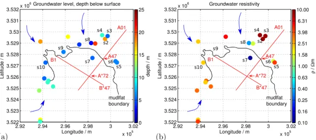
4.4 Groundwater level and resistivity at different wells . . . . 37

4.5 Comparison of (non-) deconvolved and merged NT/ZT TEM data . 43 4.6 Comparison of Gain settings and Tx-Rx polarity effect . . . . 44

4.7 Distribution of all Tx-50 sounding data and errors . . . . 46

4.8 Profile A, Tx-50: TEM transients for three soundings . . . . 49

4.9 Profile A, Tx-50: TEM ρ _a,lt data pseudosection . . . . 49

4.10 Profile A, Tx-100: TEM transients for three soundings . . . . 50

4.11 Profile A, Tx-100: TEM ρ _a,lt data pseudosection . . . . 50

4.12 Profile B, Tx-50 and Tx-100: TEM transients for three soundings . . 51

4.13 Profile B, Tx-50 and Tx-100: TEM ρ _a,lt data pseudosection . . . . . 51

4.14 Lithological borehole data (BT-1, BT-49) correlated with 1D models 54 4.15 Profile A, Tx-50: selected 1D inversion results . . . . 55

4.16 Profile A, Tx-50: quasi 2D resistivity-depth sections . . . . 57

4.17 Profile A, Tx-100: selected 1D inversion results . . . . 59

4.18 Profile A, Tx-100: quasi 2D resistivity-depth sections . . . . 61

4.19 Data fit for sounding A*61 and A*67; variation of the base layer . . 62

4.20 Profile B, Tx-50/Tx-100: selected 1D inversion results . . . . 63

4.21 Profile B, Tx-50/Tx-100: quasi 2D resistivity-depth sections . . . . . 64

4.22 Data fit for sounding B*20 and B*38; variation of the base layer . . 65

4.23 Combined visualization of Profile A and B: Marquardt models . . . 67

5.1 SLDMem3t: Yee-cell and material averaging scheme . . . . 73

5.2 Components of the electric field for FD curl-curl operator . . . . 76

5.3 Grid design for a rectangular loop transmitter . . . . 81

5.4 Multi-grid solution for large time ranges . . . . 82

5.5 SLDMem3t accuracy for varying spatial grid discretization . . . . . 83

5.6 SLDMem3t accuracy for varying resistivity contrasts . . . . 84

5.7 Inaccuracies due to lateral grid discretization . . . . 85

5.8 SLDMem3t convergence control parameters . . . . 87

5.9 Errors estimated from SLDMem3t grid analysis . . . . 88

5.10 2D fault effect on synthetic TEM data, U _ind . . . . 89

5.11 2D fault effect on synthetic TEM data, ρ a,lt . . . . 90

5.12 1D inversion of synthetic 2D data, 1D stitched section . . . . 91

5.13 1D inversion of synthetic data, excluding fault affected data . . . . 91

5.14 Synthetic 2D fault analysis: approach I . . . . 93

5.15 Synthetic 2D fault analysis: approach II, TEM tipper (U _x /U _z ) . . . 93

5.16 Profile A, Tx-50: visually/manually derived 2D model . . . . 95

5.17 Profile A, Tx-50: 2D best-fit model derived from 1D Occam results . 97 5.18 Residuals, TEM-tipper for best-fit 2D Occam model . . . . 98

5.19 Data fit of best-fit 2D occam model, sounding A27, A41 and A71 . 99 5.20 1D grid check for best fit 2D occam model . . . . 100

5.21 Profile A, Tx-50: 2D best-fit model derived from 1D Marquardt results 101 5.22 2D modeling study: lateral extent and resistivity of base . . . . 101

5.23 Data fit for sounding A49: base resistivity variation . . . . 102

5.24 2D modeling study: top of base variation . . . . 102

5.25 Data fit for sounding A41: top of base variation . . . . 103

5.26 Profile A, Tx-100: 2D forward modeling study- base removal . . . . 105

5.27 Profile A, Tx-100: depth to base and resistivity variation . . . . 105

5.28 Profile A, Tx-100: data and fit for sounding A*55 and A*73 . . . . 106

5.29 Profile B, Tx-50/Tx-100: 2D modeling study . . . . 107

5.30 Profile B, Tx-50/Tx-100: data fit for sounding B*18 and B*37 . . . 108

6.1 Model parameterization for 2D inversion . . . . 118

6.2 Block model: synthetic 2D inversion . . . . 119

6.3 χ plotted against the sounding location . . . . 120

6.4 Data fit for two selected soundings . . . . 120

6.5 Inversion with a-priori information: fixed structures . . . . 121

6.6 Shallow basin model: Synthetic 2D inversion . . . . 122

6.7 χ plotted against the sounding location . . . . 123

6.8 Data fit for two selected soundings . . . . 123

6.9 Evolution of regularization parameters: all free . . . . 124

6.10 Inversion results for fixed ration λ _x /λ _z of reg. pars. . . . 125

6.11 Evolution of reg. pars.: ratio λ x /λ z fixed . . . . 125

6.12 Inversion results with large initial reg. par. . . . 126

6.13 Inversion results for different model parameterizations . . . . 126

6.14 2D inversion Tx-50 soundings, profile A: homogeneous starting models 128 6.15 Data fit for two selected soundings . . . . 128

6.16 Comparion of three selected soundings with the 1D models . . . . . 129

6.17 2D inversion of Tx-50 soundings, profile A: ρ _a,lt -starting model . . . 131

6.18 Data fit for two three selected soundings . . . . 132

6.19 2D inversion Tx-50 soundings, profile A: fine parameterization . . . 133

6.20 Data residuals and distribution . . . . 134

6.21 Data fit for three selected soundings . . . . 135

6.22 Evolution of regularization parameters . . . . 135

List of Figures VII

6.23 Computation time per iteration . . . . 136

6.24 2D inversion of Tx-100 soundings, profile A . . . . 137

6.25 Data fit for three selected soundings . . . . 138

A.1 lithological borehole data . . . . 159

A.2 generalized composite lithological section . . . . 160

A.3 Distribution of Tx-100 sounding data points and stacking errors . . 161

A.4 1D joint inversion result for sounding A12 and A25 . . . . 173

A.5 Profile A: 1D models A01–A15 . . . . 174

A.6 Profile A: 1D models B16–B30 . . . . 175

A.7 Profile A: 1D models A31–A45 . . . . 176

A.8 Profile A: 1D models A46–A55* . . . . 177

A.9 Profile A: 1D models A56–A65* . . . . 178

A.10 Profile A: 1D models A66–A78* . . . . 179

A.11 Profile A: 1D models A79*–A80* . . . . 180

A.12 Profile B: 1D models B01–B15 . . . . 181

A.13 Profile B: 1D models B16–B30 . . . . 182

A.14 Profile B: 1D models B31*–B45* . . . . 183

A.15 Profile B: 1D models B46*–B47* . . . . 184

A.16 Quasi 2D resistivity-depth sections for Occam R2 results . . . . 184

A.17 Combined interpretation of Profile A and B: 1D Occam models . . . 185

A.18 ERT 2D inversion results: ERT-A1 to A5 . . . . 186

A.19 ERT field data pseudosections: ERT-A1 to A5 . . . . 187

A.20 2D best-fit Occam model: joined resistivities . . . . 188

A.21 Residual plots for the 2D best-fit Occam model . . . . 189

A.22 Synthetic 2D inversion using large errors for late times . . . . 190

A.23 2D inversion Tx-50 soundings: ρ _a,lt starting model . . . . 190

List of Tables

2.1 Basic quantities used in electrodynamic theory . . . . 6

2.2 Typical resistivities of selected earth materials . . . . 7

4.1 Groundwater level and electrical resistivity of well sample . . . . 37

4.2 Investigated TEM profiles . . . . 40

4.3 Investigated ERT profiles . . . . 40

A.1 Profile B: TEM sounding locations and coordinates . . . . 155

A.2 Profile A: TEM sounding locations and coordinates . . . . 156

A.3 ERT profile locations and coordinates . . . . 157

CHAPTER 1

Introduction

The focus of this thesis is the geophysical exploration of the central part of the Azraq basin in the northeastern desert of Jordan. In addition to common 1D inversion tech- niques, further 2D forward modeling strategies and a rarely used 2D inverse modeling scheme are applied to transient electromagnetic data.

The Azraq area is of potential interest for palaeoclimatical and archaeological research in the frame of the interdisciplinary Collaborative Research Centre 806, entitled Our Way to Europe (CRC 806). The CRC 806 investigates the history of modern human, particularly population movements in the past 190,000 years before present. It is de- signed to capture the complex nature of dispersal of modern man from Africa to Western Eurasia and particularly to Europe [CRC-806, 2012]. The project investi- gates various sites in the source areas, along corridors and in target areas of population movements. The Jordan rift valley in the Eastern Mediterranean served as one pos- sible corridor of dispersal of modern man [CRC-806, 2012]. A key issue addressed by the CRC 806, is the reconstruction of the palaeoclimatical conditions in the research areas and in the concerned time range. Very promising archives for a paleoclimatical reconstruction are sedimentary deposits accumulated in dry lakes. The area around the (former) oasis Qa’ Al Azraq has been a major spot for prehistoric settlements and was subject to long-term archaeological research [Stanley Price & Garrard, 1975; Copeland, 1988; Byrd, 1988]. It is a unique wetland with pools and marshes located in a large arid environment. In the basin center, a 10× 10 km ² mudflat developed consisting thick sedimentary deposits.

The geophysical investigation presented in this thesis provides the basis for probable future drilling projects within the CRC 806. Information about the subsurface are important to avoid elaborate and costly abortive drilling. The main objective is to investigate the subsurface electrical resistivity structure and particularly to identify the thickness of sedimentary deposits in the central Azraq basin area. The early work of El-Kaysi & Talat [1996] and El-Waheidi et al. [1992] provided information about the thickness of the mudflat deposits, but complete and densely investigated transects using modern geophysical equipment are not available.

To achieve the objective within the CRC 806, a 7 km and a 5 km long transects were

investigated from the periphery to the center of the mudflat depression. An extensive

survey was conducted consisting of 150 recorded central loop transient electromagnetic

(TEM) soundings. Additionally, the electrical resistivity tomography (ERT) was ap- plied as a complementary method to validate the TEM results.

The TEM mehod is often used for the investigation of shallow sedimentary basins and valley structures [Jørgensen et al., 2003; Danielsen et al., 2003; Steuer et al., 2009].

Moreover, Electromagnetic methods, particularly TEM, are widely used for ground- water studies and aquifer characterization, for example contamination and salinization problems [Fitterman & Stewart, 1986; Goldman & Neubauer, 1994; Tezkan, 1999; Yo- geshwar et al., 2012; Papen et al., 2013]. Fundamental overviews of the TEM method are given in [Nabighian & Macnae, 1991; Spies & Frischknecht, 1991] and in several comprehensive reviews related to near surface applications of electromagnetic tech- niques [Goldman & Neubauer, 1994; Tezkan, 1999; Pellerin, 2002; Auken et al., 2006;

Everett, 2011].

In the first part of the thesis, electrical resistivity-depth models are derived along both transects. Common 1D TEM data inversion algorithms are applied and the un- certainties of the models are discussed in detail on the basis of equivalent modeling and parameter importances. The 1D inverse models are patched together to quasi 2D resistivity-depth sections. Furthermore, these sections are put in context with the avail- able geological information and correlated with lithological borehole data.

As stated by Goldman et al. [1994], the conventional 1D interpretation of TEM data by 1D layered earth models has proved feasibility in numerous case studies. There- fore, TEM data is often interpreted by 1D inversion or quasi 2D/3D schemes. A quasi 2D laterally constraint inversion (LCI) was presented by Auken & Christensen [2004], where 1D sounding models are linked together along a profile line. Viezzoli et al. [2008]

extended the LCI to a quasi 3D inversion, which is called spatially constraint inver- sion (SCI). However, there are cases where distortion effects have to be considered and the field data can neither be explained by 1D models nor by quasi 2D/3D schemes [Newman et al., 1987; Goldman et al., 1994]. Although no clear distortion effects are visible in the TEM sounding data recorded in Azraq, the subsurface resistivity varies significantly along both investigated transects. For this reason, it is questionable if a 1D interpretation is adequate. Therefore, the second part of this thesis concentrates on the 2D forward and inverse modeling of the TEM sounding data. An elaborate 2D modeling study is performed to validate the subsurface resistivity structure, which is derived from prior 1D inversion results. The 2D TEM forward modeling utilizes the time domain finite difference algorithm SLDMem3t [Druskin & Knizhnermann, 1988, 1994, 1999]. It has been successfully applied to numerous forward modeling studies in 2D/3D involving time domain electromagnetic methods for various source configurations [Hördt, 1992;

Hördt et al., 1992, 2000; Hördt & Müller, 2000; Goldman et al., 2011; Sudha et al., 2011; Rödder & Tezkan, 2013].

Forward modeling approaches are always based on a prior selection of a model. Partic-

ularly, in 2D/3D a full and random parameter study involves far too many calculations,

which is not feasible. As a result, the 2D modeling results are to some extent biased

and do not provide an independent validation of the electrical resistivity-depth struc-

ture. To carry out an independent validation, a large number of TEM soundings are

inverted using the 2D iterative Gauss-Newton inversion algorithm SINV , which utilizes

the SLDMem3t as forward solver [Scholl et al., 2004; Martin, 2009]. Earlier, Commer

[2003] applied SINV to mountainous long offset transient electromagnetic (LOTEM)

1.1 This thesis 3 data from Mount Merapi, Indonesia. He used a Marquardt-type restricted 3D inversion with only a few model parameters. Scholl et al. [2004] and Martin [2009] applied the 2D inversion algorithm to LOTEM data from the Araba fault, Jordan. The derived 2D models were in good agreement with the magnetotelluric result presented by Ritter et al. [2003]. Koch et al. [2004] presented a 2D inversion of central loop TEM data using an early version of SINV . Recently, Martin [2009] extended SINV to a large scale 3D inversion scheme and successfully applied it to synthetic in-loop TEM data generated from a 3D buried conductor model. Nevertheless, SINV was not yet routinely utilized for the 2D inversion of TEM data. Therefore, the capabilities of the algorithm are pre- sented in detail and studied on the basis of synthetic models. Finally, SINV is applied to the TEM field data to validate the resistivity-depth structure derived from the 1D inverse models.

The multi-dimensional inversion of time domain electromagnetic data is not state of the art, yet. It is still a computational expensive task and the availability of large scale algorithms is limited. Over the past ten years 3D time domain inversion schemes were presented by few authors, e.g. Haber et al. [2007]; Commer & Newman [2008]; Olden- burg et al. [2013]. Recent reviews on 2D/3D numerical forward and inverse modeling for time and frequency domain electromagnetic methods were given by Newman &

Commer [2005]; Avdeev [2005]; Börner [2010].

Due to the groundwater problematic in Azraq, an additional motivation evolved during this thesis. The Azraq area is of enormous economical importance to Jordan. Approxi- mately one third of the freshwater supply for Jordan’s capital city of Amman is provided from the Azraq [Ibrahim, 1996]. The extensive groundwater exploitation has led to a severe decline in the groundwater table. In the central part of the area the groundwater is hyper-saline. To ensure the freshwater supply, groundwater research has been (and still is) an ongoing and relevant issue over the past 30 years. Several authors used geo- physical techniques to investigate the saline groundwater zone [El-Waheidi et al., 1992;

El-Kaysi & Talat, 1996; El-Naqa, 2010; Abu Rajab & El-naqa, 2013]. The geophysical investigations can support the ongoing groundwater management in the area because information about the extent of the saline water body can be derived from the results presented in this thesis.

1.1 This thesis

An introduction to the theoretical and conceptual background of the central loop transient electromagnetic (TEM) method is given in chapter 2. The basic theory of geophysical data inversion, which is indispensable in most geophysical interpretation approaches, will be introduced in chapter 3.

The survey area in the central part of the Azraq basin, Jordan and the geological

background is briefly introduced in chapter 4. The objectives of the geophysical in-

vestigations are formulated according to the regional geology and the scope of the

CRC 806. Moreover, the survey design and the processing of TEM field data is dis-

cussed. The results obtained by conventional 1D inversion are presented as quasi 2D

resistivity-depth sections and the reliability of the derived models is discussed in de-

tail. At the end of chapter 4, the geological information is integrated into the quasi

resistivity-depth sections.

In chapter 5, the theory to the 3D time domain finite difference forward solver SLD- Mem3t is explained. Important aspects of the numerical solver are discussed and an extended analysis on the calculation grid is presented. The grid design is particularly important to obtain a stable and accurate solution for the 2D forward with SLDMem3t and the inverse modeling with SINV . Moreover, a large number of soundings are inter- preted by means of 2D forward modeling and a systematic modeling study is performed to validate the subsurface resistivity structure along both transects.

The Gauss-Newton 2D inversion scheme SINV is presented in chapter 6. To investigate the capabilities of the algorithm, it is studied on the basis of two synthetic 2D models.

Finally, the subsurface resistivity-depth structure in the Azraq area is independently validated by applying the 2D inversion to the TEM field data.

Chapter 7 briefly summarizes the results of this thesis. Conclusions are drawn and an outlook for future work is given.

1.2 Preliminary notes

The survey was split into two parts. A 50 × 50 m ² transmitter loop (Tx-50) was used during the first survey in 2011, whereas a 100×100 m ² transmitter (Tx-100) was utilized in 2012. Since a lot of work was done during these two surveys, this chronology is also reflected in the presentation of the results. Sounding locations recorded with the Tx-50 setup are labeled for example A27, whereas the Tx-100 soundings are marked with an asterisk, e.g. A*80.

Vectors are presented in lower case, bold-italic characters. An exception are the vector

fields E, D, H and B, which are displayed similar to matrices in upper case, bold-

italic characters. The time derivative of the magnetic field (∂ _t B) is termed as induced ˙

voltage (U _ind ) or simply voltage (U ). Moreover, the displayed TEM data are normalized

to transmitter current I and receiver moment A _Rx . They are given in the unit V/Am ² .

The electrical resistivity ρ is simply termed as resistivity.

CHAPTER 2

The transient electromagnetic method

Electromagnetic (EM) geophysical induction methods are used to gain information of the earths subsurface structure. They are based on the phenomenon of interaction of time varying electromagnetic source fields with the physical properties of the earth.

The methods are divided into frequency and time domain electromagnetic methods.

The application of EM methods, using artificial sources, ranges from very shallow ex- ploration, e.g. archeological artifacts and unexplored ordnance detection at a few meter depths, down to several kilometers for hydrocarbon exploration in the oil/gas industry and mineral exploration. Over the past decades EM methods are widely used for envi- ronmental and engineering purposes, such as waste site exploration and groundwater studies at depths down to a few hundred meters. Several comprehensive reviews related to near surface applications of electromagnetic techniques in the time and frequency do- main were published, e.g Goldman & Neubauer [1994]; Tezkan [1999]; Pellerin [2002];

Auken et al. [2006]; Everett [2011]. The central or in-loop transient electromagnetic (TEM) method operates in the time domain. A transient earth response is measured at distinct time gates after switching off a primary source field in the transmitter. The electrical resistivity distribution mainly determines the diffusion process of the tran- sient EM fields into the ground.

The theoretical basics, which are required to understand the interaction between con- ductive media and EM-fields, are introduced in this chapter. Specific attention is paid to the description of the TEM method and its characteristic features. These descriptions follow the fundamental work of Ward & Hohmann [1991], Nabighian & Macnae [1991]

and Spies & Frischknecht [1991]. The electrical resistivity tomography (ERT) method was applied supplementary to TEM. Therefore, the theory to the ERT method is not presented, but can be found in Knödel et al. [2005] or Telford et al. [1990]. The prin- ciples of classical Electrodynamics are found in the standard work of Jackson [1975].

Table 2.1 summarizes the basic variables and quantities used in this chapter.

2.1 Electrical conduction mechanism

EM geophysical induction methods involve the measurement of electric current flow in

the conductive earth. Therefore, the electrical resistivity (ρ = 1/σ) of the ground is

crucial. For near surface materials it varies from 0.1 to 10,000 Ωm [Auken et al., 2006].

Table 2.1: Basic variables and constants used in electrodynamics. Vectors are presented as bold characters. They are given in the International System of Units (SI).

Meaning Symbol SI Unit

electric field intensity E ^V _m

electric displacement field (flux density) D ^As _m

magnetic field (flux density) B T = Vs

m

magnetic field intensity H ^A _m

current density j _m ^A

electric charge density q ^As _m

electrical permittivity ε = ε ₀ ε _{r Vm} ^As

electrical permittivity of free space ε ₀ = 8.845 · 10 ⁻¹² _Vm ^As

relative dielectric permittivity ε r non-dimensional

magnetic permeability µ = µ ₀ µ _{r Am} ^Vs

permeability of free space µ ₀ = 4π · 10 ⁻⁷ _Am ^Vs

relative permeability µ r non-dimensional

electrical conductivity σ _m ^S = A

Vm

electrical resistivity ρ Ωm = Vm

A

angular frequency ω = 2πf ¹ _s

frequency f ¹ _s

Electric current j propagates prevalently in three ways in the earth [Telford et al., 1990; Knödel et al., 2005]:

The electronic conduction prevails if a material exhibits free electrons. In most cases the electronic conduction of the rock matrix is negligible. Exceptions are found for rocks that contain high conductive minerals.

Often rocks are porous and the pores may be filled with fluids containing free ions, leading to electrolytic conduction. The resistivity varies with the mobility and con- centration of the dissolved ions [Telford et al., 1990]. These ions can originate for example from dissolved salts or contaminents. Hence, the rocks become electrolytic conductors, where the current propagates by ionic conduction. The well known empir- ical formula of Archie [1942] relates the bulk/effective resistivity with the resistivity of the pore fluid. The classical formula applies for clean and particularly clay-free (partly) saturated rocks.

The interaction between ions in the pore fluid and negative surface charges of the rock matrix causes an electric double layer at the interface. The concentration of mobile ions increases towards the double layer. The net result is an increased surface conduc- tivity, which is referred to as double layer conduction [Ward, 1990a]. Clay minerals exhibit this property to a high degree, because they have a high ion exchange capacity.

Therefore, very low resistivity values may occur for wet clay. However, if the pore fluid is high conductive the electrolytic conduction prevails [Ward, 1990a].

In case of EM geophysical induction methods at low frequencies and moderate resis-

2.2 Maxwell’s equations 7 tivities the dielectric conduction is negligible compared to the other conduction mechanisms. Therefore, the relative electric permittivity ε _r is not considered. Another material property is the relative magnetic permeability µ _r . For most earth materials µ _r is around one.

Table 2.2 summarizes the resistivity of some earth materials. Of particular interest is basalt, sandstone/limestone, clay and sand because these materials are common in the study area. The clay and water content are key parameters. Fresh to brackish and saline groundwater occurs at shallow depths and significantly determines the subsur- face resistivity.

Table 2.2: Typical resistiv- ity ranges of some earth ma- terials which occur in the survey area, Azraq. Values taken from Ward [1990a] and Palacky [1991].

material resistivity range ρ in Ωm clay ≈1 (wet) — 100 (dry clay)

shale ≈5 — 30

sandstone ≈40 — 10 ³

limestone ≈ 10 ³ — 10 ⁵

gravel and sand ≈500 — 10 ⁴

basalt ≈10 — 10 ⁵

salt water ≈0.3 — 1

fresh water ≈2 — 100

2.2 Maxwell’s equations

The interaction of electromagnetic fields and matter is based on the four Maxwell’s equations and the constitutive relations. Maxwell’s equations form a system of coupled first order linear differential equations. In differential and integral form they read as follows:

∇ · D = q

Z

S

D · dS = Z

V

q dV (2.1a)

∇ · B = 0

Z

S

B · dS = 0 (2.1b)

∇ × H = ∂D

∂t + j

I

l

H · dl = Z

S

j + ∂D

∂t

· dS (2.1c)

∇ × E = − ∂B

∂t

I

l

E · dl = − Z

S

∂ B

∂t · dS (2.1d)

The basic quantities and units are summarized in table 2.1. The integral form of

Maxwell’s equations are derived from the differential form using Gauss’ and Stokes

theorem [Jackson, 1975]. Gauss law in Eg. (2.1a) states that the charge density q are

the sources of the electric (displacement) field D. On the contrary, the magnetic flux

density B is source free, which follows from Gauss law for magnetic fields in equa-

tion (2.1b). Amperè’s law is given in equation (2.1c) and may be illustrated by a line

carrying the current density j, which causes a circulating magnetic field H. Likewise,

a time varying electrical (displacement) field D supports a circulating magnetic field.

The first type of current flow j is often called ohmic or galvanic, while the second type of current is called displacement current ∂ _t D. According to Faraday’s law of induc- tion in equation (2.1d), a time varying magnetic field B causes a circulating electric field E of opposite sign.

The last two Maxwell’s equations (2.1c) and (2.1d) are of particular importance and characterize the EM field behavior well for geophysical induction methods. However, these equations do not have any obvious relationship to matter as such, e.g. the earth physical properties [Keller, 1987]. But, the equations may be coupled with matter via the constitutive relations

B = µH and D = εE (2.2)

and Ohm’s law for isotropic media

j = σE. (2.3)

Where σ is the electrical conductivity of the medium. Ohm’s law relates the current density j to the electric field intensity E and is the most important constitutive equa- tion in terms of geophysical induction methods. In general σ, µ and ε are tensors, depending on space, time or frequency, temperature and pressure. For isotropic media they reduce to scalar quantities. Moreover, for most earth materials the magnetic per- meability µ equals the vacuum permeability µ ₀ .

2.2.1 Telegraph and Helmholtz equation

Outside of any external sources and in regions of homogeneous conductivity no free charges exist and the electrical field intensity E is source free, hence ∇·E = 0. Likewise, the current density is source free in homogeneous regions and ∇ · j = 0. By taking the curl of Faraday’s law (2.1d) and substituting ∇ × B with Amperè’s law (2.1c) a decoupled second order differential equation is obtained for E. An identical equation is derived for H in the same manner [Ward & Hohmann, 1991]. They are referred to as wave or telegraph equations ¹ :

∆F − µσ ∂

∂t F − µε ∂ ²

∂t ² F = 0 F ∈ {E, H}. (2.4) The wave equation may be transformed into the frequency domain by a Fourier trans- formation with respect to time (∂ _t → iω):

∆F − iωµσF

| {z }

conduction

+ µεω ² F

| {z }

displacement

= 0 F ∈ {E, H}. (2.5)

This equation is known as the Helmholtz equation with the wavenumber k, which implies the physical properties of the media: k ² = µεω ² − iµσω.

1 The vector identity ∇ × ∇ × F = ∇∇ · F − ∆F is used

2.2 Maxwell’s equations 9

2.2.2 Quasi static approximation

For most earth material conductivities and operating frequencies (sampling rates) of systems used for geophysical induction methods the conduction currents (σE) are much larger than the displacement currents (∂ t D). Therefore, it is µεω ² µσω in equation (2.5). Thus, in the quasi static approximation the Telegraph equation (2.4) and Helmholtz equation (2.5) reduce to:

∆F − µσ∂ t F = 0 (2.6a)

∆F − iωµσF = 0 F ∈ {E, H}. (2.6b)

These are referred to as the time and frequency domain diffusion equations. In the quasi static approximation the wavenumber is:

k = p

−iµσω = (1 − i)

r µσω

2 . (2.7)

In very resistive environments (e.g. over crystalline bedrock) and high operating fre- quencies (sampling rates) the approximation is not valid. Radiomagnetotelluric sys- tems operate up to 1 MHz and do not necessarily obey the diffusion equation in very high resistive environments [Persson & Pedersen, 2002; Kalscheuer et al., 2008]. Then, electrical displacement currents occurring as polarization effects in matter have to be considered. Ground penetrating radar is an exception, where the wave nature is part of the technique and the full wave equation needs to be solved.

Plane wave solution for a uniform conductor

One basic solution of equation (2.6a) is a positive downward decaying EM field with a harmonic time dependence e ^iωt in a uniform conductor with conductivity σ [Ward &

Hohmann, 1991]:

F(z, t) = F ⁺ ₀ e ^iωt e ^−ikz

= F ⁺ ₀ e ^iωt e ⁻ⁱ

√

2

z

e ⁻

√

2

z F ∈ {E, H}. (2.8) F ⁺ ₀ is the initial amplitude of the EM field and the wavenumber k is given in equa- tion (2.7). The initial amplitude F ⁺ ₀ is damped with depth z. In conducting media, the EM wave reduces its amplitude by a factor 1/e at a depth

δ F D = r 2

µσω . (2.9)

This is referred to as the frequency domain skin depth.

Step excitation solution for a uniform conductor

Following Ward & Hohmann [1991], the basic solution of the time domain diffusion equation (2.6b), which gives useful insights into the transient behavior of EM fields in media, is for an impulse EM field at time t = 0 in the plane z = 0:

E(z, t) H(z, t)

=

E ⁺ ₀ H ⁺ ₀

√ µσz 2π

t

e ⁻

2

4t

. (2.10)

The depth z _max := δ _{T D} at which the EM fields obtain their maximum for a fixed time t > 0 is calculated by taking the derivative with respect to z and equating to zero:

δ _{T D} = r 2t

µσ . (2.11)

This is referred to as the diffusion depth for time domain soundings. The skin depth is proportional to p

1/ω, whereas the diffusion depth is proportional to √

t. By forming the time derivative of δ T D the propagation velocity v of the EM-field maximum is obtained:

v = ∂ _t δ _{T D} = 1

√ 2µσt . (2.12)

For a fixed time t the diffusion depth is decreased in a good conductor compared to a poor conductor. Likewise, the diffusion velocity is reduced.

2.3 Central loop transient electromagnetics

There are many configurations used to carry out time domain electromagnetic (TDEM) measurements. A very common setup for deeper exploration is that of a prolonged grounded bipole transmitter, where components of the electrical and magnetic fields are recorded at a certain distance broadside or inline of the transmitter. This is of- ten referred to as the long offset transient electromagnetic method (LOTEM). For shallow investigations it is very popular to use a loop source instead of a grounded wire. A magnetometer, an induction coil or a wire loop can be used as receivers for recording the vertical component of the magnetic field (or its time derivative). If one is particularly interested in multi-dimensional subsurface structures, a three component receiver may be used. If the receiver is placed in the center of the transmitter loop it is referred to as central loop or in-loop, if placed outside it is called separate loop.

Soundings carried out with a loop source are referred to as SHOTEM (short offset transient electromagnetic method) or simply TEM. In contrast to LOTEM the closed transmitter-loop is ungrounded and acts as an inductive source. A constant current flows in the loop and is interrupted instantly at time t ₀ (step function excitation).

Due to the abrupt change of the primary magnetic field, eddy currents are induced in the conductive ground. The induced current system preserves the collapsing pri- mary field and will counter act the current switch-off. Directly after switch-off at t ⁺ ₀ the current is confined to the vicinity of the transmitter loop and is an exact mirror- image of the current in the transmitter loop before switch-off. Due to Ohmic loss, the induced surface currents dissipate into the conductive ground with progressing time [Nabighian & Macnae, 1991]. Fig. 2.1(a) illustrates the downward and outward diffu- sion of the current system for three times after current switch-off in the transmitter.

Nabighian [1979] described this concept as “smoke rings blown by the transmitter”.

For a uniform or layered halfspace the induced current system will flow in horizon-

tal planes. Hence no vertical component of the electric field E or current density j

exists. This is a direct consequence of the resistivity contrast and EM boundary con-

ditions at the air-earth interface, which applies for any inductive source hosted at

2.3 Central loop transient electromagnetics 11

(a) (b)

Figure 2.1: (a) System of equivalent current filaments over a conductive earth at three times after current switch-off in a transmitter loop. (b) Magnetic field lines and equivalent current filament for one particular time after current switch-off. Both figures are after Nabighian &

Macnae [1991].

the surface [Nabighian & Macnae, 1991]. Such a pure horizontal electric field is re- ferred to as TE-mode (tangential electric) and is of pure toroidal shape. The magnetic field sketched in Fig. 2.1(b) is induced by the equivalent current filament and pure poloidal. Nabighian [1979] showed that for a uniform halfspace the equivalent current

low resistivity high

resistivity (a)

(b)

Figure 2.2: (a) Transmitter current waveform I(t) for a 50% duty cycle. (b) Induced voltage in a receiver loop over a low and high resis- tive subsurface. T r is the ramp-time and t i the distinct acquisition times. Modified from Asten [1987].

filament diffuses downwards at an angle of approximately 47 ^◦ . It has twice the velocity v of the actual current system (cf. equation (2.12)), which diffuses at a smaller angle of 30 ^◦ .

In Fig. 2.2(a) a typical transmitter cur- rent waveform I(t) with a 50% duty cycle is illustrated. The direct current is either positive +I ₀ or negative −I ₀ before switch-off at t ₀ . One cycle pe- riod T implies two current switch-off and two switch-on pulses. As illustrated, the switch-on is technically not realized that fast as the switch-off and thus often not evaluated. Fig. 2.2(b) displays two pos- sible transients, recorded after current switch-off at distinct time gates t i in a receiver located in the center of the trans- mitter. In a high resistive environment, the decay is much steeper than in a low resistive environment. If an induction coil or a wire loop receiver is used instead of a magne- tometer, the measured quantity is the induced voltage U _ind (t):

U ind = −∂ t

Z

A

BndA rx . (2.13)

A _rx is the receiver area and n is the surface normal. Before current switch-off the mag-

netic flux through A _rx is constant and the voltage response U _ind is zero. Measurements

of the magnetic field are referred to as step response and the measurements of its time

derivative (or voltage) are called impulse response. In addition to the induced surface

current counteracting the current switch-off, the transmitter system and loop act as own inductive circuit. As a consequence the current switch-off is not instant at t ₀ . The finite switch-off time is called ramp time T _r and has to be considered at the stage of field data processing (or inversion). Its treatment is explained in section 4.5.1.

Goldman & Neubauer [1994] summarized the main advantages of the TEM method:

- Relatively large investigation depths are achieved with relatively small transmit- ter loop sizes. Additionally, no galvanic ground coupling is required, which leads to a comparably fast deployment/setup of a TEM sounding station.

- The response is measured in absence of the primary field. Thus, the investigation depth depends on the transmitter moment (transmitter size and current) and acquisition time.

- Very sensitive to conductive targets.

- The current system is focused under the transmitter, which leads to a superior depth-to-lateral investigation ratio. Therefore, TEM measurements can be inter- preted better by 1D layered earth models than other configurations, e.g. LOTEM [Spies & Frischknecht, 1991].

2.3.1 Solution for a uniform conducting halfspace

Analytical transient solutions, due to a step excitation, exist for the special case of a uniform conducting halfspace and simplified sources. Assume a large horizontal loop with radius a and current I located at z = 0. In the far zone the response of a large circular loop is to a good approximation similar to that of a vertical magnetic dipole (VMD) with moment m = Iπa ² . According to Ward & Hohmann [1991], the vertical component of the magnetic field H ˙ _z at the center of the loop is given by:

H ˙ _z = −I σµ ₀ a ³

3erf (Θa) − 2

√ π Θa(3 + 2Θ ² a ² )e ^(Θ

^a

⁾

, (2.14)

where Θ = ^{√ 1}

2δ

= p _µσ

4t . The Gauss’ error function is defined as erf (x) = 2

√ π Z x

0

e ^−τ

dτ. (2.15)

For a rectangular transmitter-loop with area A _rx an equivalent radius ˜ a = p

A/π may be used. Several other approximations for various transmitter-receiver configurations are found in Spies & Frischknecht [1991]. For theoretical derivations it is referred to Ward & Hohmann [1991] or Keller [1987].

Early and late time approximations

There are two common approximations, which reduce equation (2.14) to simple rela- tions between H ˙ _z and the subsurface resistivity ρ = 1/σ. If the transmitter radius a is much larger than the diffusion depth δ _{T D} , it is referred to as far zone sounding. Then the induction number β = a/δ _{T D} is larger than √

10 [Spies, 1989]. This is usually the

2.3 Central loop transient electromagnetics 13 case for early times after current switch-off. For t → 0 (and Θ → ∞) the Gauss’ error function approaches unity and e ^−Θ

^a

vanishes. Equation (2.14) simplifies to

H ˙ _z,et = − 3I

σa ³ , (2.16)

where H ˙ _z,et is proportional to the uniform halfspace resistivity ρ = 1/σ. The second approximation to equation (2.14) is that for late time stages t → ∞ (and Θ → 0) the error-function vanishes and e ^−Θ

^a

approaches unity:

H ˙ _z,lt = − Ia ² 20 √

π (µσ)

t ⁻

(2.17)

At late times the transient decays proportional to t ⁻

and σ

. This approximation is valid for near zone soundings, where the induction number is less than one: β = _δ ^a

T D

< 1 [Spies & Frischknecht, 1991].

Apparent resistivity

The resistivity of a homogenous halfspace, which produces the observed data for each discrete time point separately is defined as the apparent resistivity ρ _a . Equation (2.16) may be rearranged to solve for ρ, which is then referred to as early time apparent resistivity:

ρ _a,et = − a ³ 3I

H ˙ _z,et . (2.18)

Likewise, a late time apparent resistivity ρ _a,lt is obtained by rearranging equation (2.17):

10

10

10

10

10

10

10

10

10

10

10

10

time / s ρ

/ Ω m

ρ

ρ

far-zone near-zone

Figure 2.3: Early ρ _a,et and late time ap- proximations ρ a,lt for a uniform halfspace with 10 Ωm. The gray dotted lines mark the near and far zone boundaries.

ρ a,lt = − Ia ³

20 √ π

t ⁻

µ H ˙ ⁻

2 3

z,et . (2.19) Outside the near and far zone ranges, the apparent resistivity does not reflect the true earth resistivity at all [Spies & Frischknecht, 1991]. However, both transformations are useful as they provide an initial feeling for the resistivity structure and generate a first guess for automatic inversion schemes [Raiche, 1983]. Particularly the late time ap- proximation ρ _a,lt is useful, because it reduces the large dynamic range of the TEM transient.

To illustrate that, ρ _a,et and ρ _a,lt are plotted in

Fig. 2.3 for a 10 Ωm uniform halfspace. Whilst

ρ _a,et varies over seven decades of magnitude,

ρ _a,lt only varies over three decades. Up to 5 µs

the far zone assumption is valid and ρ _a,et complies with the 10 Ωm halfspace resistiv-

ity. The same applies for ρ _a,lt in the near zone for times larger than 50 µs, where ρ _a,lt

approaches the true halfspace resistivity. For intermediate times both approximations

differ significantly from the true resistivity. Any assumptions based on these approxi- mations should be drawn carefully to avoid miss-interpretation. On the one hand there is the well known over- and undershoot phenomenon, which may lead to a false in- terpretation [Raiche, 1983; Goldman et al., 1994]. On the other hand, the apparent resistivity is dual-valued and the criteria for evaluation is upon the interpreter. An- other problem is that ρ _a,lt does not reflect the resolution capability of the utilized TEM receiver system, because ρ _a,lt is not the measured quantity. Likewise, the noise mea- surements cannot be transformed. For further details it is referred to Spies & Eggers [1986], who briefly summarized the use and miss-use of apparent resistivity in electro- magnetic methods.

In this thesis, often the induced voltage is presented because it is the measured quantity and used as input for the applied inversion schemes. Since the geophysical target in the survey area is a resistor at depth occurring at late times, ρ a,lt is utilized in addition to visualize the TEM data. Furthermore, it is used to derive a-priori information for the 2D inversion scheme presented in chapter 6.

2.3.2 Solution for a 1D layered halfspace

The conventional 1D interpretation of central loop TEM data by a 1D layered subsur- face has proved feasible in many field applications [Goldman et al., 1994]. As stated earlier, the method has a superior depth-to-lateral investigation ratio and is more easily interpreted in one dimension than other TDEM configurations, e.g. LOTEM [Spies &

Frischknecht, 1991]. The derivations for a 1D layered halfspace are quite elaborate and briefly discussed in Ward & Hohmann [1991] on the basis of Schelkunoff vector poten- tials. Weidelt [1986] formulated the theory on the basis of two scalar Debye potentials.

The induced voltage U z,ind obtained in a receiver loop with area A rx generated by a horizontal electric dipole (HED) sourced at z = 0 and dipole moment D ₀ = Idl is given by

U _z,ind (t, r) = 1 2π

Z ∞

−∞

µA _rx e ^iωt D ₀ sin φ 4π

Z ∞ 0

B _E (k) − k

B _E (k) + k kJ ₁ (kr)dkdω. (2.20)

Figure 2.4: Elemen- tary dipoles forming a transmitter.

B _E (k) is the reciprocal impedance obtained at the surface, k is the wavenumber and J ₁ is the first order first kind Bessel function. The receiver loop is located at a distance r and angle φ from the dipole (cf. Fig. 2.4). The solution for a rectangular transmitter loop is obtained by superposition of the response of several elementary dipoles with moment m = Idl. In order to achieve an accurate approximate solution, the length of the el- ementary dipoles dl is determined by the induction number (i.e transmitter-receiver separation/loop size and diffusion depth).

In the near zone more dipoles are required than for far zone soundings. Equation (2.20) is solved only for one dipole and all other solutions are calculated by a coordinate transformation [Rätz, 2000]. Alternatively, the transmitter loop may also be constructed by superposi- tion of the solutions calculated for elementary vertical magnetic dipoles [Weidelt, 1986].

The first approach is implemented in the applied inversion-algorithm EMUPLUS, which

2.3 Central loop transient electromagnetics 15 is used for the 1D inversions of the TEM field data. Equation (2.20) cannot be solved analytical, since it involves the calculation of a Bessel integral of the form

g(r) = Z ∞

0

f(k)J _ν (kr)dk, ν = 1. (2.21)

Due to the oscillating nature of the Bessel function J 1 (kr) for large arguments kr, the numerical evaluation is difficult and requires very small integration steps [Weidelt, 1986]. If f(k) is sufficiently smooth, the evaluation can be accelerated by using a fast Hankel transformation. The logarithmic transformation

x := ln(r/r ₀ ) ⇔ r = r ₀ e ^x and y := −ln(kr) ⇔ k = 1 r e ^−y

are introduced, where r ₀ is a reference length. The substitution of the transformation pair into equation (2.21) yields

rg(r 0 e ^x )

| {z }

:=G(x)

= − Z ∞

−∞

f( 1 r e ^−y )

| {z }

:=F (y)

J 1 ( r ₀

r e ^x−y ) r ₀ r e ^x−y

| {z }

:= ˜ H(x−y)

dy, (2.22)

which is a convolution integral. However, H(x ˜ − y) is still a strong oscillating function, but it may be replaced by a low-pass filtered version. The numerical evaluation of equa- tion (2.22) is done by using appropriate filter coefficients for H(x−y). Filter coefficients with ten coefficients per decade are given in Weidelt [1986]. Further explanations to the fast Hankel transformation and the solutions for different dipole sources, as well as for other field components than H _z , are given in Weidelt [1986], Martin [2009] or Petry [1987].

2.3.3 Depth of investigation

The TDEM diffusion depth δ _{T D} is often used to determine the depth at which a layer is detectable for a fixed time point and overburden conductivity. But, the diffusion depth is in practice not the same as the exploration depth. A common estimate for the exploration depth or depth of investigation (doi ) for central loop TEM soundings in the near zone (late times) was suggested by Spies [1989]:

δ _doi ≈ 0.55

IA _{T x} ρ ¯ η ν

, (2.23)

where A _{T x} is the size of the transmitter loop and η _ν is the voltage noise level. A typical η _ν -value for TEM soundings is 0.5 nV /m ² . Moreover, the doi depends on the average resistivity ρ ¯ of the overburden with z ≤ δ _doi :

¯ ρ = 1

δ doi

Z δ

z=0

ρ(z)dz. (2.24)

Equation (2.23) may be used prior to a field campaign, to estimate suitable config-

uration parameters such as transmitter size and current. The δ _doi -value may also be

estimated from final 1D inversion models and plotted as a lower depth bound, which is done in this thesis. Then η _ν corresponds to the induced voltage value of the last recorded time point at each sounding. A drawback is that the doi is easily over-estimated. For example if a poor resolved deep layer exhibits large resistivities, ρ ¯ becomes large as well. Therefore, the δ _doi -value is considered as a rough and additional estimate. In ac- cordance to an example discussed by Spies [1989] and to avoid overestimation only 70%

of δ _doi is considered as the exploration depth in this thesis. Likewise to the maximum doi, a minimum doi is defined by the earliest acquisition time. For depths less than the minimum diffusion depth δ _{T D} (t _min ) only the bulk resistivity is resolved.

Particularly, for frequency domain soundings Spies [1989] suggested 1.5 · δ _{F D} as a rea- sonable estimate of the doi, where δ _{F D} is the skin depth in equation (2.9). This value is used to derive an approximate exploration depth from the 2D TEM inversion in chap- ter 6. Moreover, the skin depth δ _{F D} is used as a measure to define extremal bounds for model and grid parameterizations (cf. Hördt [1992]; Martin [2009]).

2.3.4 2D conductivity structures

If loop source TDEM measurements are conducted over essentially multidimensional structures, significant inaccuracies may ocur, when 1D interpretation schemes are ap- plied [Newman et al., 1987; Goldman et al., 1994]. For the previously discussed 1D conductivity distributions the induced currents flow in subsurface horizontal planes and the electric field is pure toroidal. Since the EM fields migrate faster in the resistor and are decelerated in a conductor, lateral subsurface variations cause the EM field to become distorted. The symmetry with respect to the transmitter is lost. Hence, both toroidal and poloidal electric fields are generated.

To illustrate the diffusion process in two dimensions, contour lines of the induced elec- tric field E are displayed in Fig. 2.5 at four times after current switch-off in a 50×50 m ² transmitter loop. The oberservation plane is a xz-slice at y = 0 m in the center of the transmitter. The model is 2D with a vertical boundary at x = 25 m. Left of the bound- ary the model has three horizontal layers (ρ 1−3 = 13, 4.5, 80 Ωm) and to the right it is homogeneous with ρ = 0.3 Ωm. The transmitter is placed on the edge of the vertical boundary.

Similar to the “smoke ring” concept of Nabighian [1979], the maximum of the electric field diffuses down- and outwards from the transmitter. Until t = 10 ⁻⁴ s the maximum of E follows roughly the red dashed line with 30 degree slope. At later times, the maximum of E prevalently migrates outwards and resides in the good conductive layer before it penetrates the resistor at depth. Right of the fault, the diffusion velocity is significantly decelerated and the maximum of E migrates slower. As a consequence, the whole current system is distorted and not anymore in an horizontal plane.

As illustrated previously in Fig. 2.1(b) the resulting magnetic field is pure poloidal in

the 1D case and symmetrical with respect to the transmitter. Thus only a vertical

magnetic field component H _z exists in the center. In case of the 2D distorted current

system in Fig. 2.5, both components H _z and H _x are generated at the center of the

transmitter. Spies & Frischknecht [1991] suggested that the ratio of H _x to H _z may be