A Study on Dust Dry Deposition: Wind-tunnel Experiment and Improved Parameterization

A Study on Dust Dry Deposition:

Wind-tunnel Experiment and Improved Parameterization

Inaugural-Dissertation zur

Erlangung des Doktorgrades

der Mathematisch-Naturwissenschaftlichen Fakultät der Universität zu Köln

vorgelegt von

Jie Zhang aus Suzhou, China

Köln 2013

Berichterstatter: Prof. Dr. Y. Shao

Prof. Dr. S. Crewell

Tag der mündlichen Prüfung: 28.10.2013

Kurzfassung

Die Staubdeposition ist eine Schlüsselkomponente des Staubzyklus, allerdings sind die Depositionsmechanismen noch nicht vollständig verstanden. Dies limitiert die Fortentwicklung der Staubforschung. Die Hauptaspekte dieser Studie sind daher die Gewinnung verlässlicher Daten zur trockenen Deposition von Staubpartikeln, die Validierung existierender Staubdepositionsschemata sowie die Verbesserung der Parametrisierung der Staubdepositionsprozesse.

Zu diesem Zweck wurde eine Reihe von Experimenten im Windtunnel durchge- führt. Um Geschwindigkeit und Größe der Staubpartikel festzustellen, die den Messbereich passierten, wurde eine laserbasierte PDPA („Phase Doppler Particle Analyzer“) Technik angewandt. Mit Hilfe eines Aerosolspektrometers wurde die Staubkonzentration gemessen. Wind- und Turbulenzmessungen wurden mit einem Schallanemometer und weiteren im Windtunnel üblichen Messgeräten durchgeführt.

Es wird außerdem eine neue Methode zur Datenverarbeitung vorgestellt. Die Staubdepositionsgeschwindigkeit wird für verschiedene Partikelgrößen, Wind- und Bodenoberflächenbedingungen auf Basis der PDPA-Daten bestimmt.

Durch die Windtunnelexperimente konnte auf diese Weise ein zuverlässiger Datensatz erstellt werden, auf dessen Grundlage zwei repräsentative Depositionssch- emata validiert werden konnten, nämlich das Schema von Slinn und Slinn (1980) für glatte Oberflächen und das Schema von Slinn (1982) für Vegetationsbedeckung. Es zeigte sich hierbei, dass die Schemata die Depositionsgeschwindigkeit insbesondere für raue Oberflächen leicht unterschätzen. Der Effekt der Interzeption hingegen wird in den Schemata deutlich unterschätzt.

Ein neues Staubdepositionsschema wird in der vorliegenden Studie vorgestellt.

Hierin wird der Zusammenhang zwischen Staubdeposition und Impulsvernichtung etabliert. Zur Beschreibung der Deposition wird die „drag partition“ Theorie inklusive der Bodenoberflächenparametrisierung eingeführt. Die verbesserte Parametrisierung kann nun sowohl auf glatte als auch auf raue Bodenoberflächen angewendet werden.

Es zeigen sich gute Übereinstimmungen der Ergebnisse des neuen Depositions-

modells mit den Windtunnelmessungen. Durch eine Sensitivitätsanalyse konnte der

neu eingeführte Oberflächenparameter, der Element-Frontalflächenindex, als vorwie-

gender Einflussfaktor auf die Kollisionseffizienz der Bodenoberfläche identifiziert

werden. Somit hat der Index starken Einfluss auf die Deposition von Partikeln aller

Größen.

Abstract

Dust deposition is a key component of the dust cycle in the Earth system. The lack of understanding for the mechanisms of dust deposition has been a major bottle neck to the development of the dust-related research field. The focus of this study is to obtain data for dust dry deposition, to validate the existing dust deposition schemes and to improve the parameterization for dust deposition processes.

A series of dust deposition experiments are carried out in a wind-tunnel laboratory.

A laser-based PDPA (Phase Doppler Particle Analyzer) technique is employed to measure the velocity and size of the dust particles which pass through the sampling area. Dust concentration is measured using an Aerosol Spectrometer and wind and turbulence are measured using a sonic anemometer and other conventional wind-tunnel instruments. A new method for processing the data is proposed. The PDPA data are used to derive the dust deposition velocity for different particle sizes and wind and surface conditions.

A reliable dataset is obtained through the wind-tunnel experiments, which are then used to validate two representative dust deposition schemes, the Slinn and Slinn (1980) scheme for smooth surfaces and the Slinn (1982) scheme for vegetation canopies. It is found that the schemes tend to underestimate dust deposition velocity, especially for rough surfaces. The effect of interception is seriously underestimated in the schemes.

A new dust deposition scheme is proposed in this study. The relationship between

dust deposition and momentum depletion is established. The drag partition theory

including the surface parameterization method is introduced to describe dust

deposition. The improved scheme is suitable for both rough and smooth surfaces. The

predictions of the new scheme are found to agree well with the experimental data. By

sensitivity analysis, it is found that the newly introduced surface parameter, element

frontal area index, has a predominant effect on surface collection efficiency and

influences the deposition of particles of all sizes.

Contents

Chapter 1 Introduction ...1

Chapter 2 Basic Theory and Study Review ...5

2.1 Basic theory ...5

2.1.1 Influencing factors...5

2.1.2 Assumptions ...8

2.1.3 Key variables...9

2.1.4 Mechanisms for dust deposition...12

2.1.5 Deposition steps ...23

2.2 Review of dust deposition experiments ...24

2.2.1 Measurement methods...24

2.2.2 Experimental data...27

2.3 Review of schemes ...29

2.3.1 Resistance model...29

2.3.2 Analytical scheme ...30

Chapter 3 Wind-tunnel Experiments...37

3.1 Introduction of the wind-tunnel experiment ...38

3.1.1 Facility and instrumentation...38

3.1.2 Purposes of the experiments...47

3.1.3 Experiment configuration and device setup ...48

3.1.4 Experimental procedure ...50

3.2 Test of the experimental conditions ...51

3.2.1 Stability and reproducibility of the environment ...51

3.2.2 Structure of wind field and dust concentration profile...53

3.3 Summary ...55

Chapter 4 Experimental Data and Scheme Validation ...57

4.1 Methodology of data processing...57

4.1.1 Processing method for deposition velocity ...57

Contents ii

4.1.2 Quality control...58

4.1.3 Method of data process ...62

4.2 Results and comparison with schemes...63

4.2.1 Dust deposition on water surface ...63

4.2.2 Dust deposition on sticky and smooth surface ...66

4.2.3 Dust deposition on low-roughness surface...68

4.2.4 Dust deposition on canopy surface...72

4.3 Conclusions...75

Chapter 5 Improved Parameterization ...77

5.1 Scheme improvement...77

5.1.1 Assumptions ...77

5.1.2 Framework of the new model...77

5.1.3 Parameterizations ...79

5.2 Scheme validation...87

5.3 Sensitivity analysis...92

5.4 Summary ...98

Chapter 6 Summary and Outlook ...99

6.1 Summary and conclusions ...99

6.2 Outlook ...101

List of Symbols ...103

Bibliography ...107

Acknowledgement ... 113

Erklärung... 115

Curriculum Vitae... 117

Chapter 1

Introduction

Dust are small mineral particles with diameter less than 20 μm. The motion of dust in the Earth system forms a dust cycle which consists of processes of dust emission, transport and deposition. Dust deposition can be divided into dry and wet deposition, depending on whether precipitation is involved in the removal process. Dust dry deposition, to be studied in this thesis in detail, refers to the removal of dust particles from atmosphere onto surface in the absence of precipitation. In addition to the effect of gravitational settling which is related to the dust particle characteristics, other factors such as atmosphere turbulences and surface properties are also important to this process. Throughout this thesis, dust dry deposition will be simply referred to as dust deposition, unless otherwise stated.

Airborne dust plays an important role in the climatic system. Dust aerosols influence the atmospheric radiation budget via scattering and absorbing shortwave and longwave radiation components (Pérez et al., 2006) and affect the optical properties and lifetime of clouds (Sokolik et al., 2001). According to the reports of the IPCC (Intergovernmental Panel for Climate Change), the uncertainty in aerosol radiative forcing is among the largest of all forcings on the climate system (IPCC Fourth Assessment Report, 2007). In addition, the transport of dust is closely related to the global cycle of minerals and nutrients. It also affects the process of soil formation (Reheis et al., 1995) and the evolution of surface topography on geological time scales (Wells et al., 1987). Moreover, airborne dust in the lower part of the atmosphere causes visibility degradations (Malm et al., 2003) and detrimental health impacts (Pope and Dockery, 1999), which strongly influence the human life.

In recent years, a number of dust models have been developed by coupling

modules for atmospheric, land-surface and aeolian processes with land-surface

parameter databases, for example, by Shao et al. (2003), Ginoux et al. (2004), Tanaka

1 Introduction 2

and Chiba (2006). One of the main research problems facing the dust modeling community is how surface dust fluxes, including emission and deposition, can be quantified through parameterization. These are both complex dynamic processes involving a number of environmental factors. Our knowledge of these processes is, however, far from complete (Shao, 2008; Petroff et al., 2008a). Dust deposition is particularly poorly understood, although the process has been studied over the last few decades by a number of research groups.

Numerous experimental studies on dust deposition have been carried out, using various measurement methods, such as collection method, gradient method and eddy correlation method. A database of experimental results of dust deposition over various surfaces and under different conditions exists (Chamberlain, 1966 and 1967;

Sehmel, 1971 and 1973; Wedding and Montgomery, 1980; Nicholson, 1993; Pryor et al., 2006 and 2007). However, a comparison of the different experimental results remains difficult due to the lack of information on detailed experimental conditions and the poor comparability between the measurement techniques (Wesely et al., 1985;

Hicks et al., 1989; Goossens and Rajot, 2008).

On the other hand, several theoretical schemes have been proposed to describe the deposition process under different situations (e.g. Bache, 1979a and 1979b; Slinn, 1982; Wesely et al., 1985; Petroff et al., 2008b). Some mechanisms including turbulence transfer, gravitational settling and surface collection are introduced to predict the quantity of dust deposited on the surface. But the disagreement between the model results and experimental data is significant (Ruijgrok et al., 1995), which indicates that these schemes still have weaknesses in accurately describing the complex deposition processes. One of the obvious deficiencies of the existing schemes is for instance that a rough surface is normally considered to consist of a uniform roughness elements and the total surface collection efficiency is based on consideration of one of the uniform roughness element. These schemes are thus difficult to apply to surfaces with multi-size roughness elements. Also the effect arising from the interactions among the roughness elements on the process of dust collection is neglected.

A thorough literature review reveals, as detailed in Chapters 2 and 3 of this thesis,

1 Introduction 3

that our knowledge of dust deposition is rather incomplete. The large uncertainties in the dust-deposition estimates in dust models, due to the lack of high quality dust-deposition data for comparison, the employment of poorly-tested dust-deposition schemes and the unreliable parameter databases required for the deposition schemes, have been a major bottle neck to the development of the entire research field.

The general aims of this study are to better understand the mechanisms of dust deposition, to collect data for dust deposition scheme validation and to develop better dust deposition schemes. The following targets are achieved through this study.

z

A series of wind-tunnel experiments on dust deposition over several surfaces is carried out and a reliable and comprehensive dataset is obtained.

z

The dataset is used to validate representative existing dust deposition schemes.

The differences between the experimental data and the scheme- predicted results are analyzed and the deficiencies of the schemes are examined.

z

An improved dust deposition scheme with a new parameterization is proposed to account for the effect of surface roughness elements interactions.

The thesis is structured as follows: Chapter 2 describes the basic theory of dust

deposition velocity, including the most important concepts and the main mechanisms

for dust deposition. The traditional experimental methods and prevalent theoretical

schemes are also described in Chapter 2. In Chapter 3, the wind-tunnel laboratory and

the equipment used for the experiment, as well as the design of the wind-tunnel

experiments, are introduced. The methodology of data processing and the

experimental data are presented in Chapter 4. Also shown in Chapter 4 is a

comparison between the measurements and the dust deposition schemes. In Chapter 5,

the new dust deposition scheme is presented and validated against the wind-tunnel

measurements. Finally, the summary of the work, along with an outlook for future

studies, is given in Chapter 6.

Chapter 2

Basic Theory and Study Review

Dust deposition as a scientific problem has attracted the attention from the environmental investigators since as early as the 1900s (Mili and Lempfert, 1904;

Winchell and Miller, 1918). In the past century, more systematic research on the topic has been carried out and a wealth of knowledge accumulated, which forms the basis of this study. In this chapter, the basic concepts and hypotheses of dust deposition will be introduced and the dust deposition mechanisms described. Theories, parameterization schemes, and experimental techniques will be reviewed.

2.1 Basic theory

2.1.1 Influencing factors

Dust deposition is the transport of dust particles from atmosphere onto earth surface.

This process is influenced by a number of factors related to the proprieties of the airborne dust particles, atmospheric flow conditions and the underlying surface characteristics.

Airborne dust

The physical properties of the airborne dust particles, including shape, size and

density, affect their dynamic behavior and hence their motion in air. As shown in

Figure 2-1, the shape of dust particles is mostly complex and irregular. Due to this fact,

the size of a dust particle is often described using an equivalent diameter (D

) which is

the diameter of a spherical object possessing the same physical property as the dust

particle (e.g., aerodynamic characteristics in the study of dust deposition). Dust

particles are therefore assumed to be spherical in many relevant theoretical works, as

2.1 Basic theory 6

well as in this study. The size of airborne dust distributes over a considerable range, from a few nanometers (nm) to several tens of micrometers (μm). The typical number and volume distributions of aerosols (including dust) are as shown in Figure 2-2.

Figure 2-1: Electron microscope images of anthropogenic (A-C) and natural airborne (D-I) particles (Gieré and Querol, 2010). Therein, D, E and F are collected from the Saharan dust.

Figure 2-2: Typical number and volume distributions of aerosols (Seinfeld and Pandis, 2012)

Another physical quantity of interest to deposition is particle density, ρ

, which

Nu mb er (dN /dl ogD

), cm

× 10

Nucleation mode

Aitken mode

Condensation mode

Accumulation mode

Droplet mode

Coarse mode Vo lu m e ( dV /dl ogD

, μ m

cm

D

(μm) 40

30 20 10 40 0 30 20 10 0

0.01 0.1 1 10

2.1 Basic theory 7

refers to the mass per unit volume of the particle itself. Particle density influences the kinetic properties of the particle and its value is dependent on the particle structure and composition. However, the density of dust particles (of quartz, clays, feldspath, calcite etc.) is typically 2650 kg·m

(Rajot et al., 2008).

The gravitational force acting on a spherical particle, G, can be calculated as g

D G =

⋅

⋅

6

1 ρ (2.1)

where g is the gravitational acceleration.

Atmosphere (air)

Drag force arising from the relative movement between air and particle is another main reason for dust motion in the atmosphere. Wind therefore plays an important role in the process of dust deposition. In neutral atmospheric boundary layers, the profile of the mean wind speed is approximately logarithmically (Shao, 2008), i.e.,

⎟⎟ ⎠

⎜⎜ ⎞

⎝

⋅ ⎛

=

0

*

ln

)

( z

z k

z u

u (2.2)

for surfaces with low roughness elements or

⎟⎟ ⎠

⎜⎜ ⎞

⎝

⋅ ⎛ −

=

0

*

ln

)

( z

z z k z u

u

(2.3)

for surfaces with high roughness elements, where u(z) is the mean wind speed (horizontal) at height z and k the von Karman constant ( ~ 0.4). The friction velocity,

u

, is defined as:

a

u ρ

= τ

*

with τ being the surface shear stress and ρ

the air density. The roughness length, z

, is

the height at which u(z) in Eq. (2.2) or (2.3) becomes zero and describes the capacity

of the surface for momentum absorption. The zero-displacement height, z

, is

introduced to describe the change of the centreoid of momentum absorption on

high-rough surface.

2.1 Basic theory 8

Surface

Both the roughness length (z

) and zero-displacement height (z

) are integral parameters related to the roughness of the surface but not the real sizes of the roughness elements (obstacles). For studying surface dust collection, the real sizes of the roughness elements need to be used. For simplicity, a roughness element is usually considered to be cylinders standing perpendicular to the ground (Figure 2-3), with h

and d

representing respectively its height and diameter.

Figure 2-3: Illustration of a roughness element.

2.1.2 Assumptions

Some assumptions are required to simplify the complex dust deposition processes and to propose feasible dust deposition schemes. The main ones commonly made in dust deposition studies are summarized in this section.

Constant flux in vertical

The most important assumption for dust deposition studies is that dust flux, i.e. mass transfer per unit area per unit time, in the atmospheric surface layer is constant in vertical. This also implies that in the absence of dust emission, the dust flux at any given height, from the top of roughness element to the reference height z

= 100z

+ z

[about 100 m for typical forest according to Businger (1986)], is equal to the dust deposition flux at the surface.

Roughness element

Ground h

d

2.1 Basic theory 9

The constant-flux assumption is not expected to hold for an instant time and location, but is tenable if dust fluxes are averaged over a sufficiently large surface for given time and/or over sufficiently long time period for given location. This assumption provides a way to establish a relationship between dust motion in air and dust deposition to the surface. It also underpins the theory for the deposition flux measurement on surface.

Surface homogeneity

The assumption of surface homogeneity is made in many dust deposition studies. The size and distribution of roughness elements on the surface are supposed to be uniform.

Furthermore, the horizontal flow field is also supposed to be homogeneous.

2.1.3 Key variables

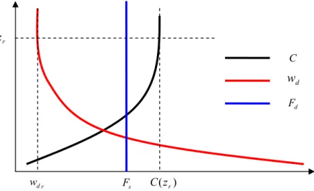
Deposition velocity

Deposition velocity, w

(z), for a given height, z, can be defined as the deposition flux, F

, normalized by the concentration, C(z), (Pryor et al., 2008):

) ) (

( C z

z F

w

= −

(2.4)

According to this definition, deposition velocity changes with dust concentration for the constant flux assumption. If dust is completely absorbed when it reaches the surface (i.e. C(0) = 0), then the deposition velocity at the surface would be infinite.

For position far away from the surface, the effect of concentration depletion is small.

This high position is normally selected as the reference height, z

. In previous studies,

deposition velocity is generally referred to w

given by Eq. (2.4) for level z

, namely

w

in Figure 2-4, unless otherwise stated. The ideal profiles of deposition velocity,

dust concentration and flux are as shown in Figure 2-4.

2.1 Basic theory 10

Figure 2-4: Idealized profiles for dust concentration, C, deposition velocity, w

, and deposition flux, F

, which is considered to be constant in vertical. F

= F

is the flux of dust deposited to the surface. Dust concentration increases with height. And hence, dust deposition velocity decreases with height. w

is the deposition velocity at reference height, z

, where the effect of concentration depletion is minimum.

Surface collection efficiency

Surface collection efficiency, ξ, is defined as (Bache, 1979a)

dose Area

dose

= Trap

ξ (2.5)

where the “trap dose” represents the number of particles deposited to a unit surface area and “area dose” refers to the number of particles flowing through an imaginary frame of unit area cross-section, perpendicular to the wind direction. This approach was originally proposed by Gregory and Stedman (1953) and then was widely applied to the studies of dust-surface interactions.

For a roughness element on rough surface, the element collection efficiency, E, represents the collected fraction of all dust particles initially moving on a collision course with the element (Figure 2-5a). The surface collection efficiency is essentially the synthesized effect of all roughness elements on the surface. The relationship between ξ and E depends on the size and location distribution of the roughness elements. If the roughness elements are uniform and distributed as shown in Figure 2-5b, the surface collection efficiency would be equal to the element collection

z

w

F

r

w

F

C ( z

)

C

2.1 Basic theory 11

efficiency, i.e. ξ = E. This situation is assumed in many existing dust deposition schemes, e.g., Slinn and Slinn (1980) (SS80 hereafter), Slinn (1982) (S82 hereafter) and Zhang et al. (2001).

Figure 2-5: Top view of surface with roughness elements. (a) Illustration of element collection efficiency. An air parcel containing dust particles moves towards a roughness element. (b) The case for equal value between surface collection efficiency and element collection efficiency, i.e.

ξ = E. (c) The case for different surface collection efficiency and element collection efficiency, i.e.

ξ < E.

In general, surface collection efficiency is contributed to several surface collection mechanisms, including Brownian motion, impaction and interception, as discussed in more detail in Section 2.1.4. We therefore have the following relationship:

) (

R ξ ξ ξ

ξ = ⋅ + + (2.6)

where ξ

, ξ

and ξ

are respectively the contribution of the Brownian motion, impaction and interception. R is a reduction factor of surface collection efficiency due to particle rebound.

Wind

Surface

Roughness element Air

parcel Roughness

element Dust

Moving direction (a)

(b)

Wind

Surface

(c)

2.1 Basic theory 12

2.1.4 Mechanisms for dust deposition

Part 1: Deposition in air

Gravitational settling

Airborne particles are forced by gravity (G, as expressed as Eq. (2.1) and shown in Figure 2-6) and move downwards. Dust deposition due to this process is called gravitational settling. For simplicity, we assume that the air is static. As a particle falls through the static air, a resisting force (f

, aerodynamic drag) occurs due to the particle-to-air relative

motion. The magnitude of the aerodynamic drag increases with the particle-to-air relative velocity, and its effect is to counteract the acceleration of gravity (Figure 2-6).

When the aerodynamic drag balances the gravity force, the particle is no longer accelerated and the particle-to-air relative velocity reaches a maximum, which is known as the particle terminal velocity.

For small spherical particles, the relationship between the aerodynamic drag and the particle-to-air relative velocity is (Hinds, 2012):

c r p

r

C

w f 3 πμ D

−

= (2.6)

where μ is the air dynamic viscosity, D

the particle diameter, w

= w

- w

the relative velocity between the particle with velocity w

and the air with velocity w. The negative sign means that the direction of the aerodynamic drag is opposed to the direction of the particle-to-air relative velocity. C

is the Cunningham correction factor which accounts for non-continuum effects when calculating the drag on small particles, which is found to be (Seinfeld and Pandis, 2012)

(

)

p

c m

e

C D λ

4 . 0 257 . 2 1

1 + +

= where

G f

w

Figure 2-6: Gravitational settling.

2.1 Basic theory 13

p D

T K

a B

m

2 π

λ =

is the particle mean free path, K

is the Boltzmann constant, T temperature, p pressure and D

the effective diameter of air molecule.

Suppose only gravity and aerodynamic forces are exerted on the airborne particle (Figure 2-6). Then, at equilibrium, we have:

= 0

=

+ G

f

(2.7)

where w

is terminal velocity, i.e. the maximum particle-to-air relative velocity a particle falling through air under gravity can reach.

A combination of Eq. (2.1), Eq. (2.6) and Eq. (2.7) leads to the expression of particle terminal velocity:

D g w

= C

⋅

μ ρ 18

2

(2.8)

In other words, if we release a particle in still air and allow it to fall over a sufficiently long time, then the final particle velocity would be

a t final

p

w w

w = + (2.9)

The first part on the right side of Eq. (2.8) is the particle relaxation time

μ τ ρ

18

2 p p c p

D

= C (2.10)

which characterizes the time required for a particle to adjust or "relax" its velocity to a new condition of forces. It follows that Eq. (2.8) can also be rewritten as

g

w

= τ

⋅ (2.11)

Diffusion

Diffusion is another important mechanism for dust transfer, which results in mixing or

mass transport without requiring bulk motion. To describe the effect of diffusion, the

quantities under consideration are separated into their mean and fluctuating

2.1 Basic theory 14

components (Stull, 2009), e.g.,

a a

a = + ′ (2.12) where a is the mean component of a and a′ the deviation of a from a . By averaging Eq. (2.12), we have

= 0

a ′ (2.13) We can now partition the quantities relevant to dust deposition as follows:

a a

a

u u

u = + ′ (2.14a)

a a

a

w w

w = + ′ (2.14b)

p p

p

w w

w = + ′ (2.14c)

C C

C = + ′ (2.14d)

where u

and w

are respectively horizontal and vertical velocity of air. The vertical dust flux averaged over a time interval can be calculated as:

C w C w F

F C C w w

F

= (

+ ′

) ⋅ ( + ′ ) =

+

=

⋅ + ′

′ (2.15) The above expression implies that the total vertical dust flux consists of two components, namely, a component of dust transport by the mean movement, F

, and a component by fluctuations or the diffusion flux, F

. Suppose the average vertical wind speed is zero. Then, the mean movement of dust is gravitational settling with flux F

, i.e.,

C w F

F

=

=

⋅ (2.16) The diffusion flux is mainly due to dust Brownian motion, F

, and air turbulence,

T

F

, i.e.,

T d B d diff

d

F F

F = + (2.17)

(a) Brownian diffusion F

Airborne dust particles are constantly and randomly bombarded from all sides by air

2.1 Basic theory 15

molecules. If the particles are sufficiently small, then the bombardments cause them to move irregularly in air, i.e. Brownian motion. Brownian motion diffuses particles from regions of higher concentration to lower. This process is termed as Brownian diffusion. The effect of Brownian diffusion can been shown experimentally to obey the Fick's Law of diffusion (Fick, 1855), i.e., the Brownian diffusion flux can be calculated by

z k C F

∂

⋅ ∂

−

= (2.18)

where

p c p B

D C T k K

πμ 3

⋅

= ⋅

is the diffusion coefficient. The negative sign means the direction of flux is opposed to the concentration gradient.

(b) Turbulent diffusion flux F

Turbulence is an important characteristic of air movement. Atmospheric turbulence can be generated by a number of different conditions, but in the atmospheric boundary layer primarily by wind shear and buoyancy. Turbulence can be visualized as consisting of irregular swirls of motion, called eddies, with different sizes and superimposed on each other (Stull, 2009).

The mechanism through which turbulence generates a dust flux is illustrated in Figure 2-7. Suppose an eddy exists near the surface as shown in Figure 2-7a. Air parcels will be exchanged between Position 1 (high level) and Position 2 (low level).

Dust particles move following the air parcels and mix with the environment. If the

average concentration at Position 1 is higher than that at Position 2, the amount of

downward moving dust particles is more than that of upward moving, i.e., dust is

transported downward by the eddy. When air parcels from Position 1 with higher

concentration ( C′ > 0) move downwards ( w′

< 0), they result in a negative flux

(downward). Likewise, the upward moving parcels ( w′

> 0), being associated with a

lower concentration ( C′ < 0), also result in a negative flux. Both the upward and

2.1 Basic theory 16

downward moving air parcels contribute to a negative w ′

C ′ . Thus, for the case shown, the average turbulent dust flux is negative.

Figure 2-7: Illustration of turbulent dust flux. Air parcels exchange places between Position 1 and 2, with more dust moving downward and less upward. As a result, dust is transferred downwards.

The above discussions suggest that eddy diffusion is determined by two factors:

particle fluctuating motion caused by turbulence and concentration gradient. This allows us to use an expression similar to Eq. (2.18) to calculate the eddy dust flux

z K C F

∂

⋅ ∂

−

= (2.19)

where K

is particle eddy diffusivity and C mean dust concentration.

For the fluctuating motion of dust particles caused by turbulence, the relationship between particle eddy diffusivity and eddy viscosity K

can be expressed as

T T

p

Sc K

K = ⋅ (2.20)

where Sc

is the turbulent Schmidt number which depends on the property of turbulence and the particle relaxation time. Csanady (1963) derived a specific

expression of Eq. (2.20) by taking the trajectory-crossing effect into consideration.

The relevant result of Csanady’s theory is

2 / 1

2 2 2

1

−

⎟ ⎟

⎠

⎞

⎜ ⎜

⎝

⎛ +

= σ

β

T

Sc w (2.21)

1 ^z

eddy

2

Net downward

dust flux

w′

− w′

1

2

C ′ >0 C ′ <0

C

w′

w′

− C

(b) Dust concentration profile

(a) Eddy

2.1 Basic theory 17

where β is a dimensionless coefficient and σ is the standard deviation of the turbulent velocity.

For a neutral atmospheric surface layer, K

is normally expressed as z

ku

K

=

(2.22)

In summary, if the vertical mean velocity of air is zero, the dust deposition flux in air consists of the following parts

C z w

K C z

k C F

F F

F

⎟⎟ ⎠ −

⋅

⎞

⎜⎜ ⎝

⎛

∂

⋅ ∂

−

⎟⎟ +

⎠

⎞

⎜⎜ ⎝

⎛

∂

⋅ ∂

−

= + +

= (2.23)

The gravitational settling flux is dependent on particulate size, density and shape, and is important in general for particles larger than 10 μm. Diffusion is effective for small particles. At relatively high levels in the atmospheric surface layer, flow is predominantly turbulent and the diffusion flux occurs mainly through eddy transfer.

Close to the surface where turbulence is weak, Brownian diffusion dominates. For particles smaller than 0.1 μm, Brownian diffusion is the dominant mechanism for dust transfer in the absence of turbulence.

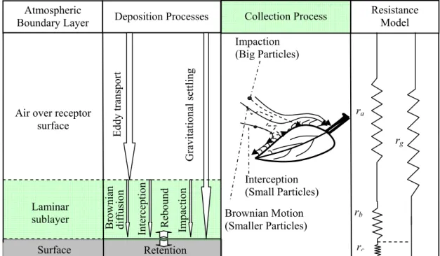
Part 2: Deposition on surface (surface collection process) Laminar layer and Quasi-laminar layer

The laminar layer as shown in Figure 2-8a is a thin layer adjacent to the surface, where turbulence is suppressed and flow is laminar. The thickness of the laminar layer, δ, over a smooth surface (small roughness-element Reynolds number) is in direct proportion to air kinematic viscosity, ν (m

s

) and inversely proportional to friction velocity, u

, (Shao, 2008), i.e.:

/

~ ν u

δ (2.24)

In the case of a rough surface, a quasi-laminar layer with thickness, δ ′ , can be

defined as a sublayer adjacent to the surface and envelops all obstacles (Figure 2-8b).

2.1 Basic theory 18

Figure 2-8: Illustration of (a) a lamina layer and (b) a quasi-laminar layer.

The particles which enter and cross the laminar layer (or quasi-laminar layer) may contact the surface and be collected. This is the so called surface collection process.

The mechanisms for surface collection include sedimentation, Brownian motion, impaction and interception. Hence, the flux of dust collected by the surface, F

, can be expressed as

in s im s B s g s

s

F F F F

F = + + + (2.25)

where F

, F

, F

, F

respectively relate to the contribution of sedimentation, Brownian motion, impaction and interception.

Sedimentation

Due to gravity, particles, especially large particles ( > 10 μm), fall through the laminar layer (or quasi-laminar layer), leading to gravitational sedimentation (Droppo, 2006).

Gravitational settling flux is independent on the type of the surface (rough or smooth) but on the surface horizontal projection area. F

can be expressed as

δ

δ

C

w

F

=

⋅ (2.26) where C

is the typical dust concentration of the laminar (or quasi- laminar) layer.

Considering the possible aggregation of hygroscopic particle in humid laminar (or quasi-laminar) layer over wet surfaces, the size of dust particle may grow to D

and

δ ,

w

is relevant terminal velocity. Methods for predicting size growth of hygroscopic particles exist (e.g. Fitzgerald, 1975; Gerber, 1985) and have been applied to dust deposition schemes (e.g. SS80; Zhang et al., 2001).

(b)

δ ^′ δ

(a)

2.1 Basic theory 19

Brownian motion

Brownian motion is the dominant mechanism for very fine particles (D

< 0.1 μm) to cross the laminar layer (Droppo, 2006). According to the definition of surface collection efficiency [i.e., Eq. (2.5)], the Brownian diffusion deposition flux can be expressed as

B a

B

s

u C

F =

⋅

⋅ ξ (2.27) where u

is the typical horizontal wind speed of the laminar (or quasi-laminar) layer.

It has been suggested that the surface collection efficiency due to Brownian motion, ξ

, can be expressed as

a B

= Sc

ξ (2.28)

where the Schmidt number Sc = ν k

is the ratio of the kinematics viscosity of air, ν , to the particle molecular diffusivity, k

. The parameter a usually lies between 1/2 and 2/3 with larger values for rougher surfaces (S82). Zhang et al. (2001) suggested a varies between 0.50 and 0.58 depending on different land-use categories.

Petroff et al. (2008b) suggested the collection efficiency for a roughness element (a cylinder perpendicular to the flow), E

, as

1 3 /

2

Re

=

B

C Sc

E (2.29)

where Re is the Reynolds number for the roughness element. C

and n

are parameters depending on flow regimes as shown in Table 2-1.

Table 2-1: Typical values of C

and n

in Eq. (2.29) for different Reynolds numbers (Petroff et al., 2008b).

Re C

n

1-4×10

0.467 1/2

4×10

-4×10

0.203 3/5

4×10

-4×10

0.025 4/5

2.1 Basic theory 20

Impaction

Suppose a dust particle moves along with the airflow near the surface. If the particle is too large to follow the directional change of the airflow, then it may collide with the surface. This process is called impaction. Particles with a diameter of 2 μm or larger can be effectively collected by impaction (Droppo, 2006). Impaction is further divided into turbulent impaction and element impaction depending on the mechanisms for the directional change of the flow, as shown in Figure 2-9.

Figure 2-9: Schematic illustration for impaction for the particles which cannot follow the flow stream line and hit the surface. Airflow is represented by the solid lines and the particle paths the dashed lines. The grayish region represents the laminar layer around the surface. (a) Turbulent impaction on smooth surface (without roughness elements). Flow direction changes due to eddy.

(b) Elemental impaction on a roughness element. Flow direction changes due to the presence of roughness element.

Turbulence is ubiquitous for atmospheric motion. A dust particle may disengage from the eddy due to inertia and hit the surface (as shown in Figure 2-9a). This is called turbulent impaction. The turbulent impaction may occur over any kind (smooth or rough) of surfaces. Similar to Eq. (2.27), the impaction deposition flux can be expressed as

im T a

im

sT

u C

F =

⋅

⋅ ξ (2.30)

where ξ

is the surface collection efficiency of turbulent impaction, which is related to dimensionless particle relaxation time (Liu and Agarwal, 1974)

ν τ τ

2

u

= ⋅

+

(2.31)

Roughness element

Side view Top view

Eddy Eddy

Wind

(a) (b)

2.1 Basic theory 21

SS80 suggested a semi-empirical formulation for surface collection efficiency as follow

− +

=

im T

ξ 10

τ (2.32)

As shown in Figure 2-9b, the direction of air flow changes near the roughness element (i.e. obstacle). The particle with big inertia may disengage from the stream line and hit the roughness element. This is called elemental impaction. The elemental impaction only occurs around the roughness element. The collection efficiency for a roughness element due to elemental impaction, E

, is normally considered as a function of the Stokes number (St). For example, S82 suggested

2 2

1 St

im

St

e

= +

ξ (2.33)

where St = τ

u

/ d

and d

is the dimension of the roughness element. Petroff et al.

(2008b) used the following form for isolated cylinders,

2

6 .

0 ⎟

⎠

⎜ ⎞

⎝

⎛

= +

St

E

St (2.34)

In summary, the surface collection efficiency caused by impaction can be expressed as )

(

im T im e im T

im

= ξ + ξ = ξ + f E

ξ (2.35)

The function f depends on the distribution of the roughness elements. For the case as shown in Figure 2-5b, f ( E

) = E

.

Interception

Interception occurs when particles of small inertia, which perfectly follow the

streamlines of the airflow, but are held back because the distance between the particle

centre and the surface is smaller than the radius (Fuchs, 1964). The predominant

collection mechanism for particles in the size range of 0.2 to 2 μm is often assumed to

be interception (Droppo, 2006).

2.1 Basic theory 22

Figure 2-10: As Figure 2-9b but is for interception. The particle follows the streamline well but contacts with the roughness element due to proximity.

Similar to impaction, interception also may be caused by air turbulence. But the particles which can follow the air well should be very small, even compared with the thickness of the laminar layer. When these small particles move into the laminar layer, they will be barely affected by the turbulence. Hence, almost no interception occurs because of turbulence, i.e. ξ

≈ 0 .

As shown in Figure 2-10. Interception mainly occurs around roughness element.

Specification of interception’s contribution to the elemental collection efficiency, E

, is unclear. The estimate is mainly based on the theoretical results for potential flows, such as (Fuchs, 1964)

c in p

e

d

E = ⋅ D 2

1 (2.36)

Similar to Eq. (2.35), the surface collection efficiency caused by interception can be expressed as

) (

in e

in

= ξ = f E

ξ (2.37)

S82 suggested the surface (vegetation) collection efficiency caused by interception as

( )

⎥ ⎥

⎦

⎤

⎢ ⎢

⎣

⎡

⋅ +

− + +

⋅

⋅

=

c p

p s

c p

p d

in v

d D c D d

D c D c

c 1

ξ (2.38)

where c

is average drag coefficient for vegetation, c

the portion of c

arising from viscous drag (as opposed to form drag), d

characteristic dimension (e.g. diameter ) of small collectors in a canopy, d

characteristic dimension of large collectors in a canopy, and c fraction of the total collected momentum collected by small collectors.

Roughness

element

Top view

2.1 Basic theory 23

Rebound

Particle rebound is possible after particle-surface collision. This phenomenon is related to the kinetic energy of the incident particle and the nature of the impact. It also depends on the adhesive conditions of the surface. It is thought to have a strong influence on the deposition of coarse particles larger than 5 μm (Chamberlain, 1967).

According to S82, the reduction in collection caused by rebound, R , can be expressed as

( ^{b St} )

R = exp − (2.39)

where b is an empirical constant, assumed to be 2 based on grass deposition measurements (Chamberlain, 1967). In the studies of Giorgi (1988) and Zhang et al., (2001), b is set to 1.

The other mechanisms, such as electrophoresis, diffusiophoresis and thermphoresis, may also contribute to dust deposition, but the magnitude is considered small compared with the ones introduced above (Davidson and Wu, 1990).

2.1.5 Deposition steps

The process of dust deposition consists of three steps, as shown in Figure 2-11.

z

Firstly, dust particles move downwards due to the combined effect of turbulent diffusion and gravitational settling from the atmosphere to a very thin layer of stagnate air adjacent to the surface.

z

Then, the particles pass through the thin laminar layer to reach the surface. In the laminar layer, turbulence is suppressed. Brownian diffusion (for small particles) and gravitational settling (for large particles) are the main factors driving the deposition process.

z

Finally, the particles are collected by the surface due to impaction, interception

and Brownian motion. They are either retained to or rebounded from the surface,

depending on a combination of surface and particle properties.

2.2 Review of dust deposition experiments 24

Figure 2-11: Dust deposition steps and mechanisms. Dust is firstly transferred downwards by eddy diffusion and gravitational settling from free air to the layer adjacent to surface. Brownian motion, interception and impaction lead to particle crossing the laminar layer to contact the surface. There, the particles are either retained or rebound.

2.2 Review of dust deposition experiments

Over the past few decades, numerous experimental studies on dust deposition have been performed. The experimental results have been summarized in the studies of McMahon and Denison (1979), Sehmel (1980), Nicholson (1988), Wesely and Hicks (2000), Pryor et al. (2008) and Petroff et al. (2008a). The measurement results are obtained under different surfaces, particles and wind conditions by using a variety of techniques. Here, the measurement methods and techniques involved are reviewed briefly.

2.2.1 Measurement methods

As stated in Eq. (2-4), dust deposition velocity, w

, is dust deposition flux divided by dust concentration. Measuring dust flux is the main challenge, for which a wide range of methods has been developed. These methods can be roughly divided into the

Resistance Model Collection Process

r

Deposition Processes

r

r

r

Laminar sublayer Air over receptor

surface

Impaction (Big Particles)

Interception (Small Particles) Brownian Motion (Smaller Particles) Atmospheric

Boundary Layer

Gravita ti ona l settl in g

Edd y tra nsp ort

Surface Retention

Brow nia n dif fusi on Interception Impact ion

Rebo un d

2.2 Review of dust deposition experiments 25

general categories of direct and indirect methods (Seinfeld and Pandis, 2012). Direct methods explicitly determine the dust deposition flux by collecting dust deposited on the surface or by measuring the vertical dust flux in air near the surface. Indirect methods derive dust deposition fluxes by measurements of quantities such as dust concentration.

Direct methods

(a) Surface collection method

Dust deposition flux is obtained by measuring the amount of dust collected by a natural or surrogate surface. The measurements are local and do not represent dust deposition over a large area unless in homogeneous conditions, but are easy to perform. A wide variety of surrogate surfaces, such as filters, plastic and glass surfaces, has been used (Goossens and Offer, 1994). Foliar extraction (e.g. leaf washing or analysis of snow) enable the natural surface to be employed in dust deposition measurements. The associated throughfall technique is widely used to measure the dust deposition on canopies (Garland, 2001).

The accumulation method and the trace method are usually used in conjunction with the surface collection method. For accumulation method, the total amount of dust deposited on the surface is collected for certain time duration. It can be readily carried out but contains no details of the measurement process, and it is not suitable for studying the influences of the meteorological conditions on dust deposition.

The tracer method is based on chemically or radioactively labeled particles, which are introduced into the field or the wind tunnel for measurement purposes. The uncertainties in aerosol granulometry and measurement reliability are usually low as the introduced aerosols are pre-characterised. This method has been widely used in wind-tunnel studies with different surface types, such as grass (Chamberlain, 1967), water (Sehmel and Sutter, 1974), moss (Clough, 1975), spruce (Ould-Dada, 2002) etc.

(b) Eddy-correlation method

Turbulent dust flux can be expressed as the covariance of particle velocity and dust

2.2 Review of dust deposition experiments 26

concentration

C w

F

= ′

′ (2.40)

For sufficiently small dust particles, w

≈ w

, such that the above equation becomes C

w

F

≈

′ ′ (2.41)

Thus, if the instantaneous wind velocity and particle concentration can be simultaneously sampled, then turbulent dust flux can be calculated by use of Eq.

(2.41). This method is called eddy-correlation method which requires fast particle sampling (Businger, 1986). To quantify the particles, various methods have been employed in the previous studies, based on analyzing the different properties of the particles, such as electric charge (Wesely et al., 1977; Lamaud et al., 1994), photometry (Hicks et al., 1982; Wesely et al., 1985; Hicks et al., 1989), optical refraction (Gallagher et al., 1997; Bleyl, 2001) or liquid condensation into nuclei or Aitken particles (Buzorius et al., 1998; Nemitz et al., 2002). Another method, termed eddy-accumulation method, operates in a similar fashion, but a distinction is made between the upward and downward moving particles (Wesely and Hicks, 2000).

Both the eddy-correlation and eddy-accumulation methods are micro- meteorological methods for measuring turbulent fluxes (Businger, 1986). But for dust flux measurements, the dust particles must be small enough, such that they behave similarly as traces in turbulent flows. As averaging over certain time duration is required to estimate the covariance, the measurement conditions must be assumed to be stationary, horizontally homogeneous and there is no particle source in the near field, such that the dust fluxes measured at a certain height can be considered to be identical to that at the surface. However, the results obtained by using this method do not include the contribution of gravitational settling.

Indirect methods (c) Gradient method

Dust deposition flux is determined by measuring the vertical gradient of dust

concentration and using the flux-gradient relationship [such as Eq. (2.19)] to infer to

2.2 Review of dust deposition experiments 27

the associated deposition flux. This method, often be used for smooth surface or low canopies, is not entirely applicable to rough canopies such as forests because the concentration gradient on the accessible measurement height is often weak, and samplers with great precision are necessary. Another limitation of this method is that the required dust diffusivity is often associated with large uncertainties (Cellier and Brunet, 1992).

2.2.2 Experimental data

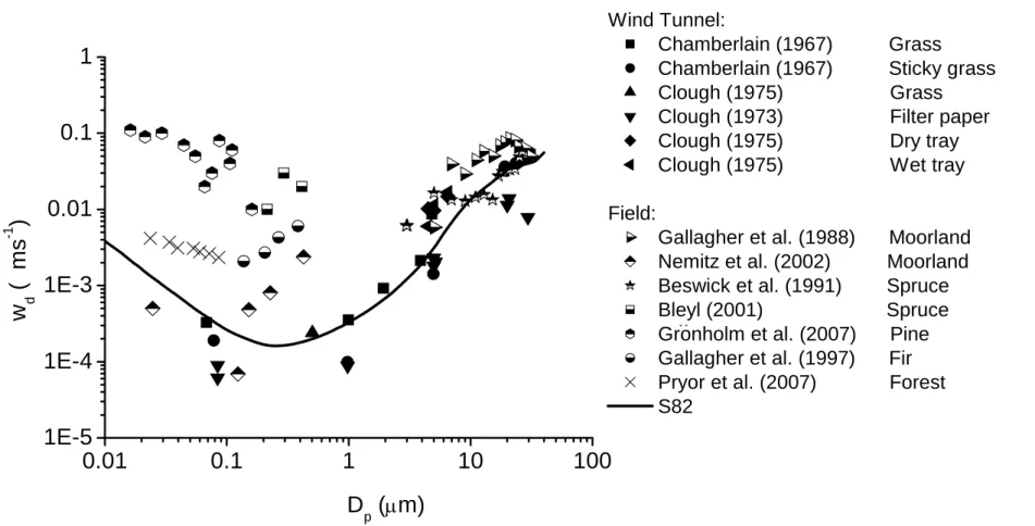
Here, we don’t repeat the work of reviewing the details of the dust-deposition experiments carried out over the past decades (McMahon and Denison, 1979;

Sehmel, 1980; Wesely and Hicks, 2000; Pryor et al., 2008; Petroff et al., 2008a), but summarize the representative results to assess the state of the existing datasets. Figure 2-12 shows the dust deposition velocity as a function of particle size for different surface types, obtained from both wind-tunnel and field experiments. The line shows the predicted results using the S82 scheme for a representative forest.

As shown, the deposition velocity for large particles exhibits a much smaller scatter and fits well to the S82 scheme. That is because gravitational settling is the main mechanism for the deposition of large particles, which depends primarily on particle size and is relatively easy to estimate. A much larger scatter in the w

measurements exists for small particles, ranging from less than 0.01 to 10 cm·s

. This wide range of variations may be related to the different experimental conditions, such as differences in meteorological conditions and surface types. It is also found that the results of field measurements are always higher than those from the wind-tunnel experiments, but detailed descriptions of the conditions for many experiments are lacking.

Different measurement methods and equipment used may be another cause for the

large scatter. The use of surrogate surfaces may lead to under-collection of depositing

particles. Further, it is questionable to extend these devices to represent the natural

surfaces. For micrometeorological techniques to work well, spatial homogeneity and

temporal stationary are assumed for the successful use of these techniques. However,

it is often difficult to fulfill all requirements in experiments under field conditions.

0.01 0.1 1 10 100 1E-5

1E-4 1E-3 0.01 0.1 1

w d (m s -1 )

Wind Tunnel:

Chamberlain (1967) Grass Chamberlain (1967) Sticky grass Clough (1975) Grass Clough (1973) Filter paper Clough (1975) Dry tray Clough (1975) Wet tray Field:

Gallagher et al. (1988) Moorland Nemitz et al. (2002) Moorland Beswick et al. (1991) Spruce Bleyl (2001) Spruce Gronholm et al. (2007) Pine Gallagher et al. (1997) Fir Pryor et al. (2007) Forest S82

D _p ( μ m)

Figure 2-12: Measurements of deposition velocities against particle size for different surfaces and a theoretic prediction.

2.3 Review of schemes 29

Besides the errors in the techniques themselves, accurate measurements of the size distribution of airborne dust was not involved in most deposition measurements.

Therefore, it cannot be ruled out that the higher deposition velocities were caused by sedimentation effects of large particles. The gap between the w

values derived from field and wind-tunnel experiments is considerable and requires further clarification.

2.3 Review of schemes

Over the past few decades, several schemes have been developed to parameterize dust deposition. A concept of deposition resistance (or its invers, the conductance) is widely applied and it has proved to be useful to interpret the deposition process in terms of an electrical resistance analogy (Hicks et al., 1987; Wesely and Hicks, 2000;

Seinfeld and Pandis, 2012).

2.3.1 Resistance model

The resistance approach uses an analogy to electrical circuits to establish a scheme that incorporates the various processes of dust deposition. The dust concentration gradient over the surface corresponds to the potential (in analogy to voltage drop) for deposition and the deposition flux is considered as current. The total deposition process is considered to function as a circuit and the deposition velocity is the inverse of the total resistance of this circuit. Following the description of the deposition mechanisms and steps, the deposition flux (like a current) flows through two parallel pathways. As shown in the right hand of Figure 2-11, the different resistances correspond to the different deposition steps. And the deposition velocity is expressed as:

t c

b a

d

r r r w

w = ( + + )

+ (2.42)

where r

is the aerodynamic resistance related to dust diffusivity and air stability.

For a neutral atmospheric boundary layer, it can be approximated as (Seinfeld and

Pandis, 2012):

2.3 Review of schemes 30

⎟⎟ ⎠

⎜⎜ ⎞

⎝

⋅ ⎛

=

0

*

1 ln z

z

r

ku (2.43)

r

represents the resistance to transfer across the laminar (or quasi-laminar) layer and is named laminar (or quasi-laminar) layer resistance. r

depends on the surface collection process and according to Zhang et al. (2001) we have

ξ ε u R r

* 0

= 1 (2.44)

where ε

is an empirical constant ( ~ 3). r

is the surface resistance defined as

d

c

F

r = C ( 0 ) (2.45)

where C ( 0 ) is the dust concentration at the surface. w

represents the contribution of gravitational settling treated as a parallel conductance (Figure 2-11).

It is usually assumed that all particles adhere to the surface (i.e., C ( 0 ) = 0 ), so that r

is normally neglected. And considering the gravitational settling is not a gradient-driven flux and does not fit into the resistance concept, a modified version of the resistance scheme is proposed by Hicks et al. (1987):

t t b a b a

d

w

w r r r

w r +

⋅

⋅ +

= + 1

(2.46)

2.3.2 Analytical scheme

The analytical scheme is generally derived from the governing equation of dust deposition [i.e. Eq. (2.23)]. The atmosphere is usually divided into several layers to describe the deposition process. The constant flux assumption and continuity of dust concentration is required to connect the adjacent layers. According to the number of the layers, the existing schemes can be categorized as a single-layer model and a multi-layer (mostly two-layer) model.

(a) Single-layer model

In a single-layer model, the surface layer is treated as a bulk entity (Owen and

Thomson, 1963; Chamberlain, 1967; Sehmel, 1980; Raupach et al., 2001). For

instance, in the Raupach et al. scheme, the deposition velocity is the bulk single-layer