equations with derivative nonlinearities
Dissertation
zur Erlangung des Grades eines Doktors der Naturwissenschaften
Dem Fachbereich Mathematik der Universit¨ at Dortmund vorgelegt von
Sebastian Herr
am 2. Mai 2006
• Prof. Dr. Herbert Koch (Universit¨ at Dortmund)
• Prof. Carlos E. Kenig, Ph.D. (University of Chicago)
Tag der m¨ undlichen Pr¨ ufung: 8. August 2006
Introduction v
1 Cauchy problems and well-posedness 1
1.1 Basic function spaces . . . . 1
1.1.1 The Fourier transformation and Sobolev spaces . . . . 2
1.1.2 The periodic case . . . . 3
1.1.3 Conventions . . . . 4
1.2 Linear equations . . . . 6
1.2.1 Linear homogeneous equations . . . . 6
1.2.2 Linear inhomogeneous equations . . . . 7
1.3 The nonlinear Cauchy problem and well-posedness . . . . 7
1.4 Analytic maps between Banach spaces . . . . 12
1.5 Notes and References . . . . 13
2 Dispersive estimates and Bourgain spaces 15 2.1 Dispersive estimates . . . . 15
2.1.1 The periodic case: The Schr¨ odinger equation . . . . . 15
2.1.2 The non-periodic case: Generalized dispersion . . . . . 16
2.2 Fourier restriction norm spaces . . . . 20
2.2.1 The periodic case: The Schr¨ odinger equation . . . . . 20
2.2.2 The non-periodic case: Benjamin-Ono type equations 27 2.3 Notes and References . . . . 33
3 Derivative nonlinear Schr¨ odinger equations 35 3.1 Motivation and main results . . . . 35
3.2 The gauge transformation . . . . 37
3.3 Multi-linear estimates . . . . 44
3.4 Proof of the well-posedness results . . . . 52
3.4.1 The gauge equivalent Cauchy problem . . . . 53
3.4.2 Proof of the main results . . . . 57
3.4.3 A Counterexample to tri-linear estimates . . . . 61
3.5 Notes and References . . . . 64
4 Benjamin-Ono type equations 67 4.1 Motivation . . . . 67
4.2 Equations of Benjamin-Ono type . . . . 68
4.2.1 A bilinear estimate . . . . 69
4.2.2 Proof of well-posedness . . . . 81
4.2.3 Sharpness of the low frequency condition . . . . 88
4.3 The Benjamin-Ono equation in the periodic case . . . . 89
4.3.1 A Counterexample to bilinear estimates . . . . 91
4.4 Equations with weak dispersion . . . . 95
4.4.1 Review of a refined energy method . . . . 96
4.5 Notes and References . . . . 99
A Auxiliary estimates 101 A.1 A Gagliardo-Nirenberg estimate in the periodic case . . . 101
A.2 An estimate involving exponentials . . . 102
A.3 An estimate for ψ . . . 103
A.4 Energy estimate for the DNLS . . . 104
A.5 Conservation laws for the DNLS . . . 105
Bibliography 116
The present work is devoted to the study of Cauchy problems for nonlinear evolution equations with initial data in Sobolev spaces of low regularity which describe the propagation of nonlinear dispersive waves.
We are interested in a well-posedness theory for these problems, i.e. for given initial data we try to find
(i) unique (ii) solutions
(iii) whose initial regularity persists
(iv) and which depend continuously on the initial data.
We are challenged to prove results with regularity assumptions on the initial data which are as weak as possible 1 . It is part of the problem to find an adequate way to express all these four aims precisely and consistently in a low regularity context.
The examples discussed here arise as one-dimensional model equations for nonlinear wave propagation in water wave theory (Benjamin-Ono type equations) or plasma physics (derivative nonlinear Schr¨ odinger equation).
In order to introduce the principle of dispersion 2 let us consider the linear equation
∂ t u + ∂ x 3 u = 0 (Airy)
We may calculate explicit solutions u : [−T, T ] × R → R with the help of Fourier analysis: Let the periodic initial datum be given by u 0 (x) = P c k e ikx , then the periodic solution is
u(t, x) = X
c k e i(kx+tk
3)
1
On the Sobolev scale H
sthis means that we try to choose s ∈ R as small as possible.
2
In the present work we focus on the analytical effects of special dispersion relations
and do not give a formal definition of dispersive waves in general cp. [Whi74], pp.363–369.
which shows that the k-th Fourier mode of the initial datum propagates with group velocity 3k 2 . The different speed of Fourier modes has certain regularizing effects such as higher integrability and in the nonperiodic case the gain of fractional derivatives in L 2 loc . On the other hand, for each t > 0 we observe ku(t)k H
s= ku 0 k H
sand the solution operator is unitary in the Sobolev spaces H s such that the solution has exactly the same regularity as the initial datum in the H s sense.
Let us consider a nonlinear version of this equation, the Korteweg-de Vries equation
∂ t u + ∂ x 3 u = ∂ x u 2 (KdV)
One idea to establish well-posedness for nonlinear equations is to apply the Picard iteration scheme to a related integral equation as in the case of or- dinary differential equations. The nonlinearity has to be small in a suitable sense such that the Duhamel term is a strict contraction and its influence on the linear solution is not too strong. To control all possible nonlinear interactions in the quadratic term and to gain the derivative one may ex- ploit the above mentioned dispersive properties of the linear equation. This strategy was used by C.E. Kenig - G. Ponce - L. Vega [KPV93c] to prove well- posedness results for (generalized) KdV equations in the non-periodic case.
In [Bou93] J. Bourgain developed a general approach to the well-posedness of nonlinear dispersive equations which reduces the problem to multi-linear estimates in spaces which are defined according to the symbol of the linear equation and inherit the dispersive properties of the solutions.
These harmonic analysis techniques in combination with the Picard it- eration found applications in many different situations and lead to strong well-posedness results in spaces of low regularity. All of them share the property that the flow map (data upon solution) is necessarily analytic 3 .
Later, it was observed that there are many interesting equations where a smooth dependence on the data or at least multi-linear estimates fail to hold [MST01, KT05b] even for regular data, although there are well-posedness results which include the continuous dependence on the data and which are based on energy type arguments.
Another approach to many nonlinear dispersive equations, such as the Korteweg-de Vries, the Benjamin-Ono or the derivative nonlinear Schr¨ odinger equation is provided by the inverse scattering theory, cp. [AC91]. However, the results in the present work do not rely on inverse scattering techniques.
Here, we are particularly interested in situations where standard multi- linear estimates for the nonlinear term cannot be true and a direct approach
3
This holds true if the nonlinear terms are analytic.
via the Picard iteration is not applicable. Our aim is to overcome these dif- ficulties by identifying the strongest interactions and modifying the method accordingly.
In Chapter 1 the basic notation and a notion of well-posedness is in- troduced. In Chapter 2 the dispersive properties of solutions to the linear equations
(∂ t − |D| α ∂ x )u = 0 in the non-periodic and
(∂ t − i∂ x 2 )u = 0
in the periodic setting as well as related function spaces are discussed.
In Chapter 3 derivative nonlinear Schr¨ odinger equations in the periodic setting are considered, in particular
∂ t u(t) − i∂ x 2 u(t) = ∂ x (|u| 2 u)(t) for t ∈ (−T, T ) u(0) = u 0
A local well-posedness result for initial data in H s ( T ) for all s ≥ 1 2 is proved which extends to global well-posedness for s ≥ 1 and data which satisfies a L 2 smallness condition, cp. [Her05a]. A detailed uniqueness statement is given and it is shown that the flow map is not uniformly continuous on balls in H s ( T ) for s ≥ 1 2 , but locally Lipschitz on subsets of data with fixed L 2 norm. Similarly, for a version of this equation with a regularized nonlinear term well-posedness follows with real analytic dependence on the intial data.
The results are shown to be sharp in certain directions.
In Chapter 4 equations of Benjamin-Ono type 4
∂ t u(t) − |D| α ∂ x u(t) + 1
2 ∂ x u 2 (t) = 0 for t ∈ (−T, T ) u(0) = u 0
are studied. Section 4.2 deals with the cases 1 < α < 2 in the non-periodic setting. Local well-posedness for initial data in spaces H (s,ω) ( R ) for s >
− 3 4 (α−1) and ω = α 1 − 1 2 and global well-posedness for real valued data in the range s ≥ 0 and ω = α 1 − 1 2 is shown, cp. [Her05b]. These spaces correspond to the usual Sobolev spaces H s ( R ) with an additional low frequency condition H ˙
−ω( R ). The result includes the analyticity of the flow map, which fails under a weaker low frequency assumption. A smoothing property is used to prove that the nonlinear equation is satisfied in the sense of distributions.
4
For α = 1 this is the Benjamin-Ono equation and for α = 2 this is the Korteweg-
de Vries equation. In the literature, these equations are known as dispersion generalized
Benjamin-Ono equations.
In Section 4.3 counterexamples are constructed which prove the failure of bilinear estimates related to the Benjamin-Ono equation (α = 1) in the peri- odic case for real valued functions with zero mean value. This complements a recent well-posedness result of L. Molinet [Mol06].
In Section 4.4 it is remarked that in the case 0 < α < 1 a slight modi- fication of the arguments of H. Koch - N. Tzvetkov [KT03b] for α = 1 also leads to well-posedness in this range.
The author is grateful to Professor Dr. Herbert Koch for the constant
support, encouragement and numerous helpful discussions. Moreover, the
author would like to thank Martin Hadac for useful remarks.
Cauchy problems and well-posedness
1.1 Basic function spaces
In this section we introduce some well-known function spaces and the Fourier transformation in order to fix notation.
We will both study problems involving functions (or distributions) on the real line being either spatially periodic or non-periodic. Let C
∞( R n ) be the linear space of infinitely differentiable functions f : R n → C and for u ∈ C
∞( R n ) we define the semi-norms
[u] α,β := sup
x∈
Rn|x α ∂ x β u(x)|
for all (multi-)indices α = (α 1 , . . . , α n ), β = (β 1 , . . . , β n ) ∈ N n 0 . We start with defining Schwartz functions.
Definition 1.1.1. We define the Fr´ echet space of smooth, rapidly decreasing functions
S( R n ) := {u ∈ C
∞( R n ) | [u] k,
Rn:= max
|α|,|β|≤k
[u] α,β < ∞, k ∈ N 0 } Definition 1.1.2. The linear space S
0( R n ) is defined as the topological dual of S( R n ). We write u(φ) = hu, φi for u ∈ S
0( R n ), φ ∈ S( R n ).
We identify f ∈ L 2 ( R n ) and ˜ f ∈ S
0( R n ), h f , φi ˜ = R
f φ dx.
1.1.1 The Fourier transformation and Sobolev spaces
Before we turn to the the definition of the L 2 based Sobolev spaces, let us quickly review the definition and basic properties of the Fourier transforma- tion.
Proposition 1.1.3. For u ∈ S( R n ) we define u(ξ) = (2π) b
−n2Z
e
−ixξu(x)dx, ξ ∈ R n (1.1) Then, b · : S( R n ) → S( R n ) is an isomorphism with inverse
ˇ
u(x) = (2π)
−n2Z
e ixξ u(ξ)dξ, x ∈ R n (1.2)
and Z
b uφdx = Z
ub φdx holds true. We define the Fourier transformation
F : S
0( R n ) → S
0( R n ), hFu, φi = hu, φi b
which is an isomorphism such that F | L
1(
Rn) and F
−1| L
1(
Rn) are given by the formulas (1.1) and (1.2), respectively.
Proposition 1.1.4. F (L 2 ( R n )) = L 2 ( R n ). Moreover, F | L
2(
Rn) : L 2 ( R n ) → L 2 ( R n ) is a unitary operator and in particular kFuk L
2(
Rn) = kuk L
2(
Rn) .
We write hxi := (1 + |x| 2 ) 1/2 and define the Bessel potential operator J s : S
0( R n ) → S
0( R n ), hFJ s u, φi = hFu, hξi s φi
Definition 1.1.5. Let s ∈ R . We define the Sobolev spaces H s ( R n ) as the space of all u ∈ S
0( R n ), such that J s u ∈ L 2 ( R n ), endowed with the norm
kuk H
s(
Rn) := kJ s uk L
2(
Rn) = Z
hξi 2s |Fu(ξ)| 2 dξ
12We remark that H s ( R n ) is a Hilbert space with scalar product (u, v) H
s(
Rn) :=
Z
hξi 2s Fu(ξ)Fv(ξ)dξ
Moreover, S( R n ) ⊂ H s ( R n ) is dense and H s ( R n ) ⊂ L 2 ( R n ) for all s ≥ 0. We
may identify H
−s( R n ) with the dual of H s ( R n ) by the Riesz representation
theorem.
1.1.2 The periodic case
We say that u ∈ S
0( R n ) is periodic, if
hu, φi = hu, φ(· + 2πk)i , k ∈ Z n
Now, the Fourier transformation of a periodic u ∈ S
0( R n ) has the follow- ing form
hFu, ψi = X
ξ∈
Zna ξ ψ(ξ)
for a unique family (a ξ ) ξ∈Z
nwhich grows at most polynomially. Hence, it is a sum of point measures and we identify a ξ and Fu(ξ), see [H¨ or83], p. 178 or [ST87], Section 3.2.
Let L 2 ( T n ) denote the Hilbert space of all f : R n → C such that f = f (· + 2πk), k ∈ Z n and f | [0,2π]
n∈ L 2 ([0, 2π] n ) with scalar product
(f, g) L
2(
Tn) = Z
[0,2π]
nf (x)g(x)dx
We identify f ∈ L 2 ( T n ) and the periodic ˜ f ∈ S
0( R n ), h f , φi ˜ = R f φ dx.
Proposition 1.1.6. F(L 2 ( T n )) = l 2 ( Z n ). Moreover, F | L
2(
Tn) : L 2 ( T n ) → l 2 ( Z n ) is unitary and in particular kF uk l
2(
Zn) = kuk L
2(
Tn) . For u ∈ L 2 ( T n ) we have
Fu(ξ) = (2π)
−n2Z
[0,2π]
nu(x)e
−ixξdx , ξ ∈ Z n
and
u(x) = (2π)
−n2X
ξ∈
ZnFu(ξ)e ixξ in L 2 ( T n )
Definition 1.1.7. Let s ∈ R . We define the Sobolev spaces H s ( T n ) as the space of all periodic u ∈ S
0( R n ), such that J s u ∈ L 2 ( T n ), endowed with the norm
kuk H
s(
Tn) := kJ s uk L
2(
Tn) =
X
ξ∈
Znhξi 2s |Fu(ξ)| 2
1 2
Notice that H s ( T n ) is a Hilbert space with scalar product (u, v) H
s(
Tn) := X
ξ∈Z
nhξi 2s Fu(ξ)Fv(ξ)
Definition 1.1.8. We define the Fr´ echet space of smooth periodic functions S ( T n ) := {u ∈ C
∞( R n ) | u = u(· + 2πz), z ∈ Z n , [u] k,
Tn:= [u] 0,k < ∞}
and of smooth functions which are spatially periodic
S( R × T n ) := {u ∈ C
∞( R n+1 ) |u(t, x) = u(t, x + 2πz), z ∈ Z n , [u] k,
R×Tn= max
k
1,|β|≤k [u] (k
1,0...,0),β < ∞, k ∈ N 0 } We observe that S ( T n ) ⊂ H s ( T n ) is dense. Moreover, H s ( T n ) ⊂ L 2 ( T n ) for all s ≥ 0. Furthermore, we may identify H
−s( T n ) with the dual of H s ( T n ) by the Riesz representation theorem.
Definition 1.1.9. The linear spaces S
0( T n ) and S
0( R × T n ) are defined as the topological duals of S( T n ) and S ( R × T n ), respectively. We write u(φ) = hu, φi.
The periodic elements of S
0( R n ) may be identified with S
0( T n ) via their Fourier representation, see [ST87], Section 3.2.3.
Definition 1.1.10. For T > 0 we define the linear spaces S T ( R n ) = {u| [−T ,T]×
Rn| u ∈ S ( R × R n )}
and
S T ( T n ) = {u| [−T ,T]×
Rn| u ∈ S ( R × T n )}
1.1.3 Conventions
In the sequel we will deal with both the spatially periodic and the non- periodic setting. At the beginning of each logical subunit we will explicitly declare the setting to avoid confusion.
There are parts where we want to treat both cases simultaniously. In this case, in order to keep the exposition short we omit the letters R and T from the above definition of the spaces. E.g. we write S for S ( R n ) and S( T n ), S T for S T ( R n ) and S T ( T n ), H s for H s ( R n ) and H s ( T n ), L p for L p ( R n ) and L p ( T n ), respectively. Moreover, dx denotes integration with respect to the Lebesgue measure on R n and its restriction to [0, 2π] n , respectively.
Similarly, dξ denotes integration with respect to the Lebesgue measure on R n and the counting measure on Z n , respectively.
As an example, the well-known Sobolev embedding and multiplication
theorems in both cases read as follows:
Proposition 1.1.11. We have
(i) H s ⊂ C k for s > k + n 2 , k ∈ N 0
(ii) H s ⊂ L p for s ≥ n 2 − n p , 2 ≤ p < ∞ (iii) L p ⊂ H s for s ≤ n 2 − n p , 1 < p ≤ 2
(iv) L 1 ⊂ H s for s < − n 2 with continuous embeddings.
We omit the proof (for the non-periodic case see [Tri83], Section 2.7.1, for the periodic case see [ST87], Section 3.5.5.).
Corollary 1.1.12. Let s ≥ 0 and assume that s [≤] < s 1 , s 2 , s
[<]
≤ s 1 + s 2 − n 2 Then, there exists c > 0 such that
ku 1 u 2 k H
s≤ cku 1 k H
s1ku 2 k H
s2, u 1 ∈ H s
1, u 2 ∈ H s
2(1.3) In particular, H s is a Banach algebra for s > n 2 .
Proof. Define v i = F
−1|Fu i |. The point-wise estimate on the Fourier side hξi s ≤ chξ 1 i s + chξ − ξ 1 i s shows
ku 1 u 2 k H
s≤ hξi s
Z
Fu 1 (ξ − ξ 1 )F u 2 (ξ 1 )dξ 1 L
2ξ
≤ckJ s v 1 v 2 k L
2+ ckv 1 J s v 2 k L
2≤ckJ s v 1 k L
p1kv 2 k L
p2+ ckv 1 k L
q1kJ s v 2 k L
q2for p 1
1
+ p 1
2
= q 1
1
+ q 1
2
= 1 2 . We start with the case s = s 1 + s 2 − n 2 . Then, necessarily 0 < s i < n 2 and we choose p 1 = s n
2
and q 2 = s n
1
and the claim follows from Proposition 1.1.11 and the fact that kv i k H
si= ku i k H
si.
In the case s < s 1 + s 2 − n 2 we use the estimate
hξi s ≤ chξ 1 i s−s
2hξ − ξ 1 i s
2+ chξ 1 i s
1hξ − ξ 1 i s−s
1and arrive at
ku 1 u 2 k H
s≤ckJ s−s
2v 1 J s
2v 2 k L
2+ ckJ s
1v 1 J s−s
1v 2 k L
2≤ckJ s−s
2v 1 k L
∞kJ s
2v 2 k L
2+ ckJ s
1v 1 k L
2kJ s−s
1v 2 k L
∞Because H s
1+s
2−s⊂ L
∞by Proposition 1.1.11 the claim follows.
1.2 Linear equations
Let s ∈ R and φ : R n → R be a continuous function of polynomial growth.
We define φ(D) to be the Fourier multiplier operator φ(D) : H s ⊃ D φ,s → H s φ(D)f = F x
−1φF x f
which has dense domain D φ,s := {f ∈ H s | hξi s φF x f ∈ L 2 }.
1.2.1 Linear homogeneous equations
Let s ∈ R , u 0 ∈ H s and define W (t)u 0 by
F x W (t)u 0 (ξ) := e itφ(ξ) F x u 0 (ξ) Then, kW (t)u 0 k H
s= ku 0 k H
sand
W (t) : H s → H s
is a well-defined, linear and isometric operator. For u 0 ∈ D φ,s the function u(t) := W (t)u 0 satisfies u ∈ C 1 ( R , H s ) and solves the Cauchy problem
∂ t u(t) − iφ(D)u(t) = 0 for t ∈ (−T, T )
u(0) = u 0 (1.4)
The following proposition summarizes important properties of W (t) (cp.
[CH98] Theorem 3.2.3).
Proposition 1.2.1. Let s ∈ R . The one-parameter family (W (t)) t∈
R⊂ L(H s ) is a group of unitary operators. Moreover,
(i) kW (t)u 0 k H
s= ku 0 k H
s, u 0 ∈ H s (ii) t 7→ W (t)u 0 ∈ C( R , H s ), u 0 ∈ H s
(iii) t 7→ W (t)u 0 ∈ C( R , D φ,s ) ∩ C 1 ( R , H s ), u 0 ∈ D φ,s
(iv) W (0) = Id, W (t + t
0) = W (t)W (t
0), W (t)
∗= W (−t) and for u 0 ∈ D φ,s the function u(t) = W (t)u 0 satisfies (1.4).
Because of its importance let us rewrite this solution for u 0 ∈ S in an explicit form
u(t, x) = W (t)u 0 (x) = (2π)
−nZ Z
e i(x−y)ξ+itφ(ξ) u 0 (y) dydξ (1.5)
Examples 1.2.2. (i) φ(ξ) = −|ξ| 2 : the equation
∂ t u(t) − i∆u(t) = 0 is called the (linear) Schr¨ odinger equation.
(ii) n = 1 and φ(ξ) = ξ 3 : The equation
∂ t u(t) + ∂ x 3 u(t) = 0 is called the Airy equation.
1.2.2 Linear inhomogeneous equations
Next, we recall Duhamel’s principle for the linear inhomogeneous problem (see [CH98], Section 4.1). Compare also Proposition 1.3.3.
Proposition 1.2.3. Let T > 0 and s ∈ R . Assume that u 0 ∈ D φ,s and f ∈ C([−T, T ], H s ) ∩ L 1 ([−T, T ], D φ,s ) as well as u ∈ C([−T, T ], D φ,s ) ∩ C 1 ((−T, T ), H s ). Then, the following statements are equivalent:
(i) u solves
∂ t u(t) − iφ(D)u(t) = f (t) , t ∈ (−T, T ) u(0) = u 0
(1.6) in H s .
(ii) u satisfies
u(t) = W (t)u 0 + Z t
0
W (t − t
0)f (t
0) dt
0, t ∈ (−T, T ) (1.7) in H s .
Remark 1.2.4. More generally, for initial data in H s and f ∈ L 1 ([−T, T ], H s ) the integral equation above defines a function u ∈ C([−T, T ], H s ).
1.3 The nonlinear Cauchy problem and well- posedness
We are interested in nonlinear Cauchy problems of the type
∂ t u(t) − iφ(D)u(t) = F (u(t)) for t ∈ (−T, T ) u(0) = u 0
(1.8)
Let us recall the four aims formulated in the introduction: For given initial data in L 2 based Sobolev spaces we try to find
(i) unique (ii) solutions
(iii) whose initial regularity persists
(iv) and which depend continuously on the initial data.
In this section we will give a precise mathematical meaning to the nonlinear Cauchy problem (1.8) and well-posedness. Since (1.8) is nonlinear and we want to study these equations in a low regularity framework, there is no unified notion of solutions like the theory of distributions provides for linear equations. To give an example, consider the Korteweg-de Vries equation
∂ t u(t) + ∂ x 3 u(t) = ∂ x u 2 (t)
for periodic initial data u 0 ∈ H s ( T ) for s < 0, where it is not clear how to define the product u · u. Nevertheless, C.E. Kenig - G. Ponce - L. Vega [KPV96] and T. Kappeler - P. Topalov [KT03a] and others derived well- posedness results in some range where the generalized solutions are defined by an extension procedure. 1
In this section we will define a rather weak general notion of well-posedness, related to [KT03a]. In each particular application considered here, we will be able to strengthen this in certain directions by using the specific structure of the problem. One main point here is the regularity of the flow map.
Examples 1.3.1. (i) In Chapter 3 we consider a Schr¨ odinger equation in one space dimension with the derivative nonlinearity
∂ t u(t) − i∂ x 2 u(t) = ∂ x (|u| 2 u)(t) (ii) The nonlinear equations in one space dimension
∂ t u(t) + ∂ x 3 u(t) = ±1
k + 1 ∂ x u k+1 (t)
are called Korteweg - de Vries equation (KdV) if k = 1, modified Korteweg - de Vries equation (mKdV) if k = 2 or generalized Korteweg - de Vries equation of order k for k ≥ 3.
1
Concerning uniqueness, cp. Remarks in [Chr05].
(iii) n = 1 and φ(ξ) = ξ|ξ|: The equations
∂ t u(t) − |D|∂ x u(t) = ±1
k + 1 ∂ x u k+1 (t)
are called Benjamin - Ono equation (BO) if k = 1, modified Benjamin - Ono equation (mBO) if k = 2 or generalized Benjamin - Ono equation of order k for k ≥ 3.
(iv) n = 1 and φ(ξ) = ξ|ξ| α , 1 < α < 2: We call
∂ t u(t) − |D| α ∂ x u(t) = ∂ x u 2 (t) equation of Benjamin - Ono type, see Chapter 4.
Assumption. Let us assume throughout this work that there exists a num- ber k ≥ 0 such that H k ⊂ D φ,0 and F : H s → H s−k is locally Lipschitz continuous for all s ≥ k.
Obviously, for functions u ∈ C([−T, T ], H k ) ∩ C 1 ((−T, T ), L 2 ) the ex- pressions
∂ t u(t) , φ(D)u(t) , F (u(t)) ∈ L 2 are well-defined for all t ∈ (−T, T ).
Definition 1.3.2. A function u ∈ C([−T, T ], H k ) is called a regular solution of (1.8), iff u ∈ C 1 ((−T, T ), L 2 ) and
∂ t u(t) − iφ(D)u(t) = F (u(t)) is fulfilled in L 2 for every t ∈ (−T, T ).
Let us review Duhamel’s principle.
Proposition 1.3.3. The following statements are equivalent:
(i) u ∈ C([−T, T ], H k ) ∩ C 1 ((−T, T ), L 2 ) is a regular solution (ii) u ∈ C([−T, T ], H k ) solves
u(t) = W (t)u(0) + Z t
0
W (t − t
0)F (u(t
0))dt
0, t ∈ (−T, T ) Proof. Assume (i). Then, for v(t) = W (−t)u(t) ∈ C 1 ((−T, T ), L 2 ) we have
∂ t v(t) = −iφ(D)W (−t)u(t) + W (−t)∂ t u(t)
= W (−t)F(u(t)), t ∈ (−T, T )
which implies
v(t) = v(0) + Z t
0
W (−t
0)F (u(t
0))dt
0and the claim (ii) follows. Now, assume (ii). Then, by assumption Z t
0
W (−t
0)F (u(t
0))dt
0∈ C 1 ((−T, T ), L 2 ) and v(t) = W (−t)u(t) ∈ C 1 ((−T, T ), L 2 ) solves
∂ t v(t) = W (−t)F(u(t)), t ∈ (−T, T ) which gives (i).
In most of the cases which are interesting to us, the existence and unique- ness of smooth solutions will be well-known (or at least straightforward to show) by classical means like a regularization procedure and energy esti- mates. However, we will not have to rely on any results about regular solu- tions 2 .
Definition 1.3.4. Let s ∈ R and H , → H s such that S ⊂ H is dense and let B R = {u 0 ∈ H | ku 0 k H < R}. We say that the Cauchy problem (1.8) is locally [globally] well-posed in H (in the minimal sense) iff there exists a non-increasing function T
∗: (0, ∞) → (0, ∞) such that for all R > 0 and 0 < T ≤ T
∗(R) [for all R > 0 and all T > 0] the following conditions are satisfied:
(i) There exists a continuous map
S R,T : B R → C([−T, T ], H)
(ii) If s
0≥ s, then S R,T (B R ∩ H s
0) ⊂ C([−T, T ], H s
0∩ H ) and S R,T | B
R∩Hs0
: B R ∩ H s
0→ C([−T, T ], H s
0∩ H ) is continuous.
(iii) There exists s 1 ≥ k such that for u 0 ∈ B R ∩ H s
1the function S R,T (u 0 ) is the unique regular solution in C([−T, T ], H ∩ H s
1) of (1.8).
The map S R,T is called the flow map or solution map.
Let M ⊂ H be an open subset. We say that the Cauchy problem is locally [globally] well-posed in H for data in M (in the minimal sense), iff (i)-(iii) hold true with B R replaced by B R ∩ M .
2
Except for Section 4.4.
Roughly speaking, we may summarize this definition of well-posedness as follows: The map data 7→ solution is well-defined for smooth data and extends to a continuous map from H ∩ H s
0to C([−T, T ], H ∩ H s
0) for all s
0≥ s.
We are mainly interested in the cases where H = H s for some s ∈ R . But sometimes, it is also interesting to consider subsets of H s endowed with slightly stronger norms, see Chapter 4.
Proposition 1.3.5. Assume that the Cauchy problem (1.8) is locally well- posed in a space H , → H s for some s ∈ R .
(i) Let R > 0, 0 < T ≤ T
∗(R) and u 0 ∈ B R . If v n → v in C([−T, T ], H) for a sequence v n ∈ C([−T, T ], H ∩ H s
1) of unique regular solutions of (1.8) with v n (0) → u 0 in H, it follows v = S R,T (u 0 ).
(ii) Assume u 0 ∈ B R
1and R 2 ≥ R 1 and let T 1 = T
∗(R 1 ). Then, for all 0 < T 2 ≤ T
∗(R 2 ) we have
S R
1,T
1(u 0 )| [−T
2,T
2] = S R
2,T
2(u 0 )
Proof. The first claim directly follows from parts (ii) and (iii) of Definition 1.3.4
v = lim
n→∞ v n = lim
n→∞ S R,T (v n (0)) = S R,T ( lim
n→∞ v n (0)) = S R,T (u 0 ) where the limits are taken in C([−T, T ], H) and H , respectively.
For the proof of the second claim it suffices to consider smooth data u 0 ∈ H ∩ H s
1by continuous dependence and density. But then the claim immediately follows from part (iii) of Definition 1.3.4.
Remark 1.3.6. We conclude that well-posedness in the minimal sense implies that there exist unique limits of smooth, regular solutions whose initial reg- ularity persists and which depend continuously on the initial data. Hence, the two aims existence and uniqueness are fulfilled in a very weak limiting sense which is inherited from existence and uniqueness for smooth, regular solutions. This is natural under the assumption we made on F which is only defined for quite smooth functions.
Remark 1.3.7. In the applications we will always try to strengthen the well-
posedness results in several directions, in particular we want to verify that
S R,T (u 0 ) fulfills the equation at least in a distributional sense and to specify
a uniqueness class. Moreover, we are interested in the regularity properties of
the flow map. All this depends mainly on suitable estimates for the nonlinear
expression.
Remark 1.3.8. We defined the time of existence only with respect to balls around the origin, such that the flow map is then defined on these balls with a common time of existence. Alternatively, one could define T
∗: H → (0, ∞]
to be a lower semi-continuous function and require that the flow maps exist locally with a common time of existence, which will not be considered here.
1.4 Analytic maps between Banach spaces
In this section we will introduce differentiability and analyticity in the infinite dimensional setting. This will be relevant when studying the regularity of the flow maps in the later applications. The aim here is to provide some well-known facts for future reference.
Let X, Y be Banach spaces over R [over C ], U ⊂ X open. We define C 1 (U, Y ) as the set of all [complex] differentiable maps F : U → Y , such that F
0: U → L(X, Y ) is continuous and inductively we define C k (U, Y ) for k = 2, . . . , ∞. Let us recall
Proposition 1.4.1. Let F : U → Y be differentiable. Assume that for u ∈ U there exists ε > 0 such that F
0: B ε (u) → L(X, Y ) is bounded. Then, F | B
ε(u) is Lipschitz continuous. In particular, if F ∈ C 1 (U, Y ), then F is locally Lipschitz continuous.
The following definition is the straightforward generalization of analytic- ity to Banach spaces.
Definition 1.4.2. Let X, Y be Banach spaces over C [over R ], U ⊂ X open and F : U → Y . Then, we say that F is analytic [real analytic], iff for every u ∈ U there exists r > 0 with B r (u) ⊂ U such that for every k ∈ N 0
there exists a continuous k-linear map L k : X × . . . × X → Y and with L (k) (x) = L k (x, . . . , x)
F (x) =
∞
X
k=0
L (k) (x − u), x ∈ B r (u) holds true with uniform convergence in B r (u).
Let us discuss two trivial examples, which will be used in the sequel.
Examples 1.4.3. Let X, Y be Banach spaces over C [over R ].
(i) Let T : X × . . . × X → Y be k-linear and continuous. Then, the map
X → X, x 7→ T (x, . . . , x) is analytic [real analytic].
(ii) Let X be a Banach algebra. The exponential map X → X, x 7→ e x is analytic [real analytic] by definition.
In the next theorem we summarize some properties of analytic maps.
Theorem 1.4.4. Let X, Y be Banach spaces over C , U ⊂ X open and F : U → Y . The following three statements are equivalent:
(i) F is analytic.
(ii) F is complex differentiable in U .
(iii) F is locally bounded and for all y
0∈ Y
0and all u ∈ U, v ∈ X the maps {z ∈ C | u + zv ∈ U } → C , z 7→ hy
0, F (u + zv)i
are analytic.
Proposition 1.4.5. Let X, Y, Z be Banach spaces over C [over R ], U ⊂ X, V ⊂ Y open and F : U → V ⊂ Y , G : V → Z analytic [real analytic].
Then, G ◦ F : U → Z is analytic [real analytic].
Finally, we state an implicit function theorem.
Theorem 1.4.6. Let k ∈ N , X, Y, Z be Banach spaces [over C ; over R ], U ⊂ X and V ⊂ Y neighborhoods of x 0 ∈ X and y 0 ∈ Y , respectively, and let F ∈ C k (U × V, Z ) [let F be analytic; let F be real analytic], such that F(x 0 , y 0 ) = 0 and D y F (x 0 , y 0 ) is invertible. Then, there exist balls B r (x 0 ) ⊂ U, B R (y 0 ) ⊂ V and exactly one map G ∈ C k (B r (x 0 ), Y ) [one analytic map G : B r (x 0 ) → Y ; one real analytic map G : B r (x 0 ) → Y ] with G(B r (x 0 )) ⊂ B R (y 0 ) such that G(x 0 ) = y 0 and F (x, G(x)) = 0 for x ∈ B r (x 0 ).
1.5 Notes and References
The contents of this chapter is well-known and can be found in several text- books, with the only exception of Section 1.3.
For rigorous definitions, identifications and further properties of the ob- jects defined in Section 1.1 we refer to the textbooks of L. H¨ ormander [H¨ or83]
(Chapter VII), W. Kaballo [Kab99] (Kapitel VII) and J. Bergh - J. L¨ ofstr¨ om
[BL76] (Chapter 6), R.J. I´ orio - V. I´ orio [II01] as well as the detailed treat-
ments of H.-J. Schmeisser - H. Triebel [ST87] (Chapter 3) and H. Triebel
[Tri83] (Chapter 2). The books of T. Cazenave - A. Haraux [CH98] and A.
Pazy [Paz83] serve as a general reference for Section 1.2 as they provide an exhaustive introduction to linear evolution equations and semi group theory.
The aim of Section 1.3 is to formulate the minimal requirements which have to be fulfilled when we want to discuss well-posed Cauchy problems in the later applications. For different notions of well-posedness and ill- posedness for dispersive equations we refer to the influential works of J.L.
Bona - R. Smith [BS75], T. Kato [Kat75, Kat83], J. Bourgain [Bou93], C.E.
Kenig - G. Ponce - L. Vega [KPV93c, KPV93a, KPV96, KPV01], L. Molinet - J.-C. Saut - N. Tzvetkov [MST01], M. Christ - J. Colliander - T. Tao [CCT03], H. Koch - N. Tzvetkov [KT05b], D. Tataru [Tat05], M. Christ [Chr05], T. Kappeler - P. Topalov [KT05b] as well as A.D. Ionescu - C.E.
Kenig [IK05]. Moreover, an overview of results on local and global well- posedness is provided by web pages maintained by J. Colliander - M. Keel - G. Staffilani - H. Takaoka - T. Tao [CKS + ].
For the contents of Section 1.4 we refer to the textbooks of J. Mujica [Muj86], Chapters I-II, IV and K. Deimling [Dei85], §7.7 and §15. For the definition of analyticity, see e.g. [Dei85], Def. 15.1 and [Muj86], Def. 5.1.
For the proof of the first part of Theorem 1.4.4 see [Muj86], Thm. 13.16
and Def. 13.1. The second part of Theorem 1.4.4 follows from combining
[Muj86], Thm. 8.12, Prop. 8.6 and Thm. 8.7. For Banach spaces over C
Proposition 1.4.5 follows from the chain rule, see [Muj86], Thm. 13.6 and
the equivalence of Theorem 1.4.4 (i) and (ii). For Banach spaces over R ,
we first complexify the spaces, extend the analytic maps to open sets of the
complex spaces and apply the result for C , similar to the process in the proof
of [Dei85], Thm. 15.3 on pp.151-152. The proof of Theorem 1.4.6 is given in
[Dei85], Thm. 15.1, Cor. 15.1 and Thm. 15.3 (a).
Dispersive estimates and Bourgain spaces
2.1 Dispersive estimates
In this section we will discuss certain space-time estimates which display the dispersive character of the equations in consideration. Although the linear solution operator W (t) is an isometry in H s , it has certain smoothing effects.
2.1.1 The periodic case: The Schr¨ odinger equation
In this subsection we recall the beautiful L 4 ( T 2 ) estimate for the Schr¨ odinger equation in the periodic case in one spatial dimension, i.e. the phase function now is φ : Z → R , φ(ξ) = −ξ 2 . The following result is due to A. Zygmund [Zyg74] (formulated as a restriction theorem for the Fourier transform), see also J. Bourgain [Bou93].
Theorem 2.1.1. Let u 0 ∈ L 2 ( T ). Then,
√ 1 2π
X
ξ∈
Ze i(ξx−tξ
2) Fu 0 (ξ) L
4(
T2
)
≤ √
42ku 0 k L
2(
T) (2.1)
Proof. Let f(t, x) =
√1
2π
P
ξ∈
Ze i(ξx−tξ
2) F u 0 (ξ). Then,
kf fk L
2(
T2) =
1 2π
X
(ξ
1,ξ
2)∈
Z2F u 0 (ξ 1 )Fu 0 (ξ 2 )e it(ξ
22−ξ21)+i(ξ
1−ξ2)x L
2(
T2
)
We rewrite this sum as a Fourier series in (t, x) variables 1
2π X
(τ,ξ)∈Z
2a(τ, ξ)e ixξ+itτ
where
a(τ, ξ) = X
(ξ
1,ξ
2)∈P(τ,ξ)
Fu 0 (ξ 1 )Fu 0 (ξ 2 )
and P (τ, ξ) = {(ξ 1 , ξ 2 ) | ξ 2 2 − ξ 2 1 = τ, ξ 1 − ξ 2 = ξ}. Now, for given pair of frequency variables (τ, ξ) 6= (0, 0) of the form (τ, ξ) = (ξ 2 2 − ξ 2 1 , ξ 1 − ξ 2 ) there is at most one solution (ξ 1 , ξ 2 ). Moreover a(0, 0) = P
ξ∈
Z|F u 0 (ξ)| 2 , and by Plancherel
kf f k L
2(
T2) =
X
(τ,ξ)∈
Z2|a(τ, ξ)| 2
1/2
≤ √ 2 X
ξ∈
Z|F u 0 (ξ)| 2
and the claim follows.
2.1.2 The non-periodic case: Generalized dispersion
In this subsection we consider the non-periodic case and the phase function φ : R → R , φ(ξ) = ξ|ξ| α for α > 0. Let W α u 0 (t, x) = W α (t)u 0 (x) be the linear group defined by
FW α (t)u 0 (ξ) = e itξ|ξ|
αFu 0 (ξ) Definition 2.1.2. Let p ∈ [4, ∞], q ∈ [2, ∞] and
2 p + 1
q = 1 2 Then (p, q) is called an admissible pair.
The following theorem is a special case of [KPV91a], Thm. 2.1.
Theorem 2.1.3. Let α > 0 and (p, q) be an admissible pair. Then we have k|D|
α−1pW α f k L
pt
L
qx≤ ckf k L
2x(2.2)
Z t 0
|D|
α−1pW α (t − s)f (s) ds L
pt
L
qx≤ ckf k L
1t
L
2x(2.3) Proof. The estimate
k|D|
α−1pW α fk L
pt
L
qx≤ ckf k L
2xdirectly follows from [KPV91a], Thm. 2.1, formula (2.3). Then, using Minkowski’s inequality,
Z t 0
|D|
α−1pW α (t − s)f (s) ds L
pt
L
qx≤
|D|
α−1pW α (t − s)f (s) L
pt
L
qxL
1s≤ c
|D|
α−1pW α (t)W α (−s)f (s) L
1s
L
ptL
qx≤ c kW α (−s)f (s)k L
1s
L
2x= ckf k L
1 tL
2xwhere we exploited (2.2) and the fact that W α (−s) is an isometry in L 2 . The next theorem, which is due to C.E. Kenig - G. Ponce - L. Vega (cp.
Lemma 2.1 in [KPV91b] or [KPV91a], Theorem 4.1) describes the sharp local smoothing effect. The proof is nothing else but a change of variables and Plancherel in t.
Theorem 2.1.4. Let α > 0. Then, for u ∈ S( R ) Z
R
||D|
α2W α (t)u 0 (x)| 2 dt = 1
1 + α ku 0 k 2 L
2, x ∈ R (2.4) which shows k|D|
α2W α u 0 k L
∞x
L
2t= q
1
1+α ku 0 k L
2.
We will now provide a useful and well-known formula for approximate identities.
Lemma 2.1.5. Let g(x) = π
−12e
−x2, g ε (x) = ε
−1g(ε
−1x) and let f ∈ L 1 ( R ) be continuous. Moreover, let ϕ : R → R be continuously differentiable. As- sume that ϕ(x) = 0, x ∈ supp(f ) iff x ∈ {x 1 , . . . , x n } and ϕ
0(x i ) 6= 0 and supp(f ) is compact or lim inf x→±∞ |ϕ(x)| > 0. Then,
ε→0 lim Z
g ε (ϕ(x))f (x) dx =
n
X
i=1
f (x i )
|ϕ
0(x i )| (2.5)
Proof. Within the support of f there are finitely many zeros of ϕ, these are simple, and ϕ stays away from zero at infinity if f is not compactly supported. Hence, there exists a δ > 0 such that with I i := (x i − δ, x i + δ)
ϕ(x) = 0, x ∈ supp(f ) ⇐⇒ x = x i , |ϕ
0(x)| ≥ c > 0 , x ∈ I i
and |ϕ(x)| ≥ c > 0 for x ∈ V := supp(f ) \
n
[
i=1
I i
Then, Z
I
ig ε (ϕ(x))f (x) dx = Z
ϕ(I
i)
g ε (y) f (ϕ|
−1I
i
(y))
|ϕ
0(ϕ|
−1I
i
(y))| dy → f (x i )
|ϕ
0(x i )| (ε → 0) because ϕ|
−1I
i
(0) = x i and (g ε ) ε>0 is an approximate identity. In V we have
Z
V
g ε (ϕ(x))f (x) dx
≤ sup
x∈V
g ε (ϕ(x)) Z
V
|f(x)| dx
≤ε
−1e
−ε−2c
2kf k L
1→ 0 (ε → 0) because |ϕ| ≥ c in V .
We will now apply this in the proof of a sharp bilinear smoothing esti- mate. Roughly speaking, the bilinear operator defined below controls α/2 derivatives on the product of two solutions at different frequency. This is particularly useful for the study of quadratic nonlinearities involving deriva- tives and it is a generalization of previous estimates for Schr¨ odinger and KdV equations by A. Gr¨ unrock [Gr¨ u01, Gr¨ u05a], which in turn were related to work by J. Bourgain [Bou98]. For δ > 0 let |x| δ := ζ(x/δ)|x| for an even function ζ ∈ C
∞with ζ| [−1,1] ≡ 0 and ζ|
R\[−2,2]≡ 1 and 0 ≤ ζ ≤ 1.
Theorem 2.1.6. We define the bilinear operator I δ s via
F x I δ s (u 1 , u 2 )(ξ) = Z
ξ=ξ
1+ξ
2|ξ 1 | 2s − |ξ 2 | 2s
1 2
δ b u 1 (ξ 1 ) u b 2 (ξ 2 ) dξ 1 . for all u 1 , u 2 ∈ S ( R ). Then, for all δ > 0
I
α 2
δ (W α u 1 , W α u 2 ) L
2xt
≤ r 2
1 + α ku 1 k L
2 xku 2 k L
2x
, (2.6)
Proof. For fixed t ∈ R we use Plancherel in x and calculate
I
α 2
δ (W α (t)u 1 , W α (t)u 2 )
2 L
2x= 1 2π
Z Z
ξ=ξ
1+ξ
2||ξ 1 | α − |ξ 2 | α | δ
12e it(ξ
1|ξ1|α+ξ
2|ξ2|α) b u 1 (ξ 1 ) u b 2 (ξ 2 ) dξ 1
2
dξ
= 1 2π
Z Z Z
e itP (ξ,ξ
1,η
1) f (ξ, ξ 1 , η 1 ) dη 1 dξ 1 dξ (2.7) with the phase function
P (ξ, ξ 1 , η 1 ) = ξ 1 |ξ 1 | α + (ξ − ξ 1 )|ξ − ξ 1 | α − η 1 |η 1 | α − (ξ − η 1 )|ξ − η 1 | α and
f (ξ, ξ 1 , η 1 )
= ||ξ 1 | α − |ξ − ξ 1 | α | δ
12||η 1 | α − |ξ − η 1 | α | δ
12u b 1 (ξ 1 ) u b 2 (ξ − ξ 1 ) u b 1 (η 1 ) u b 2 (ξ − η 1 ) For fixed ξ, ξ 1 the function P 1 (η 1 ) = P (ξ, ξ 1 , η 1 ) has only two simple roots ξ 1 , ξ − ξ 1 in the support of f . Moreover,
|P 1
0(η 1 )| = (1 + α)||ξ − η 1 | α − |η 1 | α | ≥ (1 + α)δ in supp(f ) (2.8) and
|P 1
0(ξ 1 )| = |P 1
0(ξ − ξ 1 )| = (1 + α)||ξ − ξ 1 | α − |ξ 1 | α |.
For the approximate identity (g ε ) from Lemma 2.1.5 we observe F g ε ↑ (2π)
−12. By Fubini’s theorem and the Fourier inversion formula
I(ε) := (2π)
−12Z
Fg ε (t) Z Z Z
e itP (ξ,ξ
1,η
1) f (ξ, ξ 1 , η 1 ) dη 1 dξ 1 dξdt
= Z Z Z
g ε (P (ξ, ξ 1 , η 1 ))f (ξ, ξ 1 , η 1 ) dη 1 dξ 1 dξ
Now, because of (2.8) we may use the dominated convergence theorem to show
ε→0 lim I(ε) = Z Z
ε→0 lim Z
g ε (P(ξ, ξ 1 , η 1 ))f (ξ, ξ 1 , η 1 ) dη 1 dξ 1 dξ (2.9) By Lemma 2.1.5 we conclude that this is equal to
Z Z f (ξ, ξ 1 , ξ 1 )
|P 1
0(ξ 1 )| + f (ξ, ξ 1 , ξ − ξ 1 )
|P 1
0(ξ − ξ 1 )| dξ 1 dξ
≤ 1+α 1 Z Z
| c u 1 (ξ 1 )| 2 | c u 2 (ξ − ξ 1 )| 2 + | c u 1 (ξ 1 ) c u 2 (ξ 1 )|| u c 1 (ξ − ξ 1 ) c u 2 (ξ − ξ 1 )| dξ 1 dξ
≤ 1+α 2 ku 1 k 2 L
2 xku 2 k 2 L
2x
On the other hand, by the monotone convergence theorem and (2.7) we see
ε→0 lim I(ε) =
I δ
α2(W α u 1 , W α u 2 )
2 L
2xtwhich implies (2.6).
Remark 2.1.7. The proof shows that this estimate is sharp in the sense that for u ∈ S ( R )
δ→0 lim I
α 2
δ (W α u, W α u) L
2xt
= r 2
1 + α kuk 2 L
22.2 Fourier restriction norm spaces
Now, we define function spaces which are built according to the symbol of the linear equation and therefore comprise much information about the dispersive properties of their solutions, cp. [Bou93].
We will introduce these spaces with the intention to apply the results in Chapters 3 and 4 and we will treat both cases separately, mainly be- cause of the non-standard low frequency condition used in the case of equa- tions of Benjamin-Ono type. We start with the case of the one dimensional Schr¨ odinger equation on T .
2.2.1 The periodic case: The Schr¨ odinger equation
In this subsection we consider the periodic case and the phase function φ : Z → R , φ(ξ) = −ξ 2 , associated to the Schr¨ odinger equation
∂ t u(t) − i∂ x 2 u(t) = 0
and W (t) denotes the corresponding group of unitary solution operators F x W (t)u 0 (ξ) = e
−itξ2F x u 0 (ξ)
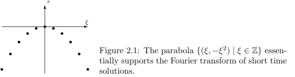
Assume that u(t, x) = χ(t)W (t)u 0 (x) where χ ∈ C 0
∞(−2, 2), χ ≡ 1 in [−1, 1], so u is a solution on [−1, 1]. Then,
Fu(τ, ξ) = χ(τ b + ξ 2 )F x u 0 (ξ)
Now, because χ b is a Schwartz function, we notice that Fu is highly localized
near the discrete parabola τ = −ξ 2 and decays in τ-direction faster than any
polynomial.
ξ τ
- 6
r r r r
r r r r
r r r
Figure 2.1: The parabola {(ξ, −ξ 2 ) | ξ ∈ Z } essen- tially supports the Fourier transform of short time solutions.
Definitions and basic properties of the spaces
The above observation motivates the following definition, which is essentially due to Bourgain [Bou93], see also [Gin96, GTV97, CKS + 04, Gr¨ u00].
Definition 2.2.1. Let s, b ∈ R . The Bourgain space X s,b associated to the Schr¨ odinger operator ∂ t − i∂ x 2 is defined as the completion of the space S( R × T ) with respect to the norm
kf k X
s,b:=
X
ξ∈Z
Z
R
hξi 2s hτ + ξ 2 i 2b |Ff (τ, ξ)| 2 dτ
1/2
(2.10)
X s,b
−is defined similarly by replacing hτ + ξ 2 i with hτ − ξ 2 i.
Moreover, Y s,b is defined as the completion of the space S( R × T ) with respect to
kf k Y
s,b:=
X
ξ∈Z
Z
R
hτ + ξ 2 i b hξi s |Ff (τ, ξ)| dτ 2
1/2
(2.11)
and the space Z s := X s,
12
∩ Y s,0 with norm kuk Z
s:= kuk X
s,1 2
+ kuk Y
s,0(2.12)
For T > 0 we define the restriction norm space Z s T := {u| [−T ,T] | u ∈ Z s } with norm
kuk Z
Ts
= inf{k uk e Z
s| u = u| e [−T ,T] , u e ∈ Z s }
We observe that the spaces X s,b and X s,b
−are isometrically isomorphic via complex conjugation kuk X
s,b= kuk X
−s,b
.
Moreover, for a function u ∈ S( R × T ) and v(t) = W (−t)u(t) we have kJ t b J x s vk 2 L
2= X
ξ∈Z
Z
hτi 2b hξi 2s |F v(τ, ξ)| 2 dτ
and
Fv(τ, ξ) = Fu(τ − ξ 2 , ξ) which shows
kJ t b J x s vk L
2= kuk X
s,bTherefore, X s,b is isometrically isomorphic to L 2 and (X s,b )
0is isometrically isomorphic to X
−s,−b. Every element of X s,b and Y s,b can be identified with a distribution in S
0( R × T ).
Lemma 2.2.2. Let s ∈ R , T > 0. S T ( T ) is a dense subset of Z s T .
Proof. Let u ∈ Z s T . There exists u e ∈ Z s such that u = u| e [−T ,T] . Because S( R × T ) ⊂ Z s is dense we find a sequence u e n ∈ S( R × T ) such that e u n → e u.
With u n = u e n | [−T ,T] it follows ku − u n k Z
Ts
≤ k˜ u − u ˜ n k Z
s→ 0 because (˜ u − u ˜ n )| [−T ,T] = u − u n .
Linear estimates
The following proposition contains the well-known and frequently used em- bedding estimates of Sobolev type.
Proposition 2.2.3.
If 2 ≤ p < ∞, b ≥ 1 2 − 1
p : kuk L
pt
H
s≤ckuk X
s,b(2.13) If 2 ≤ p, q < ∞, b ≥ 1
2 − 1
p , s ≥ 1 2 − 1
q : kuk L
pt
L
qx≤ckuk X
s,b(2.14) If 1 < p ≤ 2 , b ≤ 1
2 − 1
p : kuk X
s,b≤ckuk L
pt
H
s(2.15) We may replace X s,b by X s,b
−. Moreover,
kuk C(
R,H
s(
T)) ≤ckuk Z
s, s ∈ R (2.16) kuk Y
s,b1
≤ckuk X
s,b2
, b 2 > b 1 + 1
2 (2.17)
Proof. We consider v = W (−·)J x s u for u ∈ S( R × T ). Then, by Minkowski’s and Sobolev’s inequality
kuk L
pt
H
xs= kvk L
pt
L
2x≤ kvk L
2x
L
pt≤ ckJ t b vk L
2x
L
2t= ckuk X
s,band the claim (2.13) follows. Combining this with another application of Sobolev’s inequality in the space variable kv(t)k L
qx≤ ckJ x s v(t)k L
2x
gives (2.14). Estimate (2.15) follows by duality from (2.13). The estimates for X s,b
−follow from the invariance of L p t H x s and L p t L q x under complex conjuga- tion. To prove (2.16) it suffices to prove an estimate for the sup norm for u ∈ S( R × T ) by density. We write for t ∈ R
F x u(t, ξ) = c Z
R
e itτ F u(τ, ξ) dτ
by the Fourier inversion formula. This yields ku(t)k H
s= c
Z
R
e itτ hξi s F u(τ, ξ) dτ L
2ξ≤ ckhξi s Fu(τ, ξ)k L
2ξ
L
1τNow we take the supremum with respect to t. The last estimate follows from the Cauchy-Schwarz inequality in τ:
kuk 2 Y
s,b1
= X
ξ∈
ZZ
R
hτ + ξ 2 i b
1hξi s |Ff (τ, ξ)| dτ 2
≤ X
ξ∈
ZZ
R
hτ + ξ 2 i 2b
1−2b2dτ Z
R
hτ + ξ 2 i 2b
2hξi 2s |Ff (τ, ξ)| 2 dτ
Since by assumption 2b 1 − 2b 2 < −1, there exists c > 0, such that for all ξ Z
R
hτ + ξ 2 i 2b
1−2b2dτ ≤ c which finishes the proof.
We review the L 4 estimate from Theorem 2.1.1 as well as an L 6 estimate in the framework of X s,b due to J. Bourgain [Bou93], but in versions of A.
Gr¨ unrock [Gr¨ u00] which are global in time.
Proposition 2.2.4. For −b
0, b > 3 8 there exists c > 0, such that
kuk L
4(
R×T) ≤ ckuk X
0,b(2.18)
and its dual version
kuk X
0,b0≤ ckuk
L
43(
R×T) (2.19) hold true. Moreover, for b > 1 2 and any ε > 0 there exists c > 0, such that
kuk L
6(
R×T) ≤ ckuk X
ε,b(2.20) and its dual version hold true. Finally, for all ε > 0 and 2 ≤ p < 6 there exists c > 0 such that
kuk L
p(
R×T) ≤ ckuk X
ε,1 2(2.21) In all estimates we may replace X s,b by X s,b
−.
Proof. The estimates (2.18), (2.19) and (2.20) can be found as Lemma 2.1 and Lemma 2.2 in [Gr¨ u00]. To prove (2.21) we fix ε > 0 and 2 ≤ p < 6 and interpolate (see e.g. [Gr¨ u02] Lemma 1.4) between (2.20)
kuk L
6(
R×T) ≤ ckuk X
δ1,1 2+δ2
for small enough δ 1 , δ 2 > 0 and the trivial statement kuk L
2(
R×T) ≤ kuk X
0,0and obtain (2.21). That the estimates hold both for X s,b and X s,b
−results from the invariance of L p spaces under complex conjugation.
We summarize the behavior of the X s,b , Y s,0 norms under multiplication with cutoffs in time. Let χ ∈ C 0
∞((−2, 2)) denote a symmetric function with χ ≡ 1 in [−1, 1] and χ T (t) = χ(t/T). For the following lemma see e.g. J.
Ginibre - Y. Tsutsumi - G. Velo [GTV97], Lemma 2.5.
Lemma 2.2.5. Let s ∈ R and 0 < T ≤ 1. There exists c > 0, such that kχ T uk Y
s,0≤ ckuk Y
s,0Moreover, for 0 ≤ b 1 < b 2 < 1 2 or − 1 2 < b 1 < b 2 ≤ 0 there exists c > 0, such that
kχ T uk X
s,b1≤ cT b
2−b1kuk X
s,b2and for any δ > 0 there exists c > 0, such that kχ T uk X
s,1 2
≤ cT
−δkuk X
s,1 2