Liquidity Risk in Limit Order Book Markets

Book Markets

Inauguraldissertation

zur Erlangung des Doktorgrades

der Wirtschafts– und Sozialwissenschaftlichen Fakult¨at der Universit¨at zu K¨oln

2006

vorgelegt von

Dipl.-Kfm. Daniel Mayston

aus K¨oln

Korreferent: Prof. Dr. Heinrich Schradin

Abgabetermin der Arbeit:

02. Mai 2006

List of Figures V

List of Tables VIII

List of Abbreviations IX

List of Symbols XI

1 Introduction 1

1.1 Key Issues and Relevance . . . . 2

1.2 Contribution to the Literature . . . . 6

1.3 Main Results and Procedure . . . . 10

2 Liquidity in Limit Order Book Markets 13 2.1 Market Microstructure . . . . 13

2.1.1 Price Formation with Market Frictions . . . . 14

2.1.2 Elements of a Limit Order Book Market . . . . 18

2.2 Static Models of the Limit Order Book . . . . 21

2.2.1 Model Assumptions . . . . 21

2.2.2 Equilibrium Outcome . . . . 23

2.2.3 Implications . . . . 26

2.3 Dynamic Models of the Limit Order Book . . . . 30

2.3.1 Model Assumptions . . . . 31

2.3.2 Equilibrium Outcome . . . . 33

2.3.3 Implications . . . . 36

2.4 Conclusion . . . . 39

I

3 Market Structure and Data 43

3.1 Market Structure . . . . 43

3.1.1 Xetra Market Model . . . . 43

3.1.2 Order Types and Matching Rules . . . . 46

3.2 Data Set . . . . 49

3.2.1 Order Book Reconstruction . . . . 49

3.2.2 Descriptive Statistics . . . . 53

4 Resiliency of the Limit Order Book 61 4.1 Introduction to Resiliency . . . . 62

4.2 Construction of Liquidity Measures . . . . 69

4.3 Framework and Hypotheses . . . . 71

4.4 Dynamics of the Limit Order Book . . . . 75

4.4.1 Base Estimation of Resiliency . . . . 75

4.4.2 Order Book Tick and Time Horizon . . . . 78

4.5 Interaction of Resiliency and Microstructural Factors . . . . 81

4.5.1 Construction of Microstructure Proxies . . . . 81

4.5.2 Impact of Microstructure Proxies on Resiliency . . . . 85

4.6 Resiliency in the Cross-Section . . . . 89

4.7 Relationship with other Liquidity Measures . . . . 94

4.8 Conclusion . . . . 96

5 Commonality Across Limit Order Books 101 5.1 Introduction . . . 101

5.2 Commonality at Best Prices . . . 105

5.3 Commonality Beyond Best Prices . . . 110

5.3.1 Construction of Liquidity Measures . . . 110

5.3.2 Market Model Results . . . 113

5.3.3 Principal Components Results . . . 119

5.4 Time Variation of Commonality . . . 122

5.4.1 Time of Day . . . 123

5.4.2 Market Momentum . . . 125

5.5 Conclusion . . . 127

6 Pricing Effects of Liquidity 131

6.1 Introduction . . . 131

6.2 Liquidity Measures and Pricing Factors . . . 136

6.3 Methodology . . . 139

6.3.1 Fama-French Factors . . . 140

6.3.2 Estimation Procedure . . . 143

6.3.3 Potential Errors and Biases . . . 147

6.4 Asset Pricing Test Results . . . 148

6.4.1 Correlation Structure of Pricing Factors . . . 148

6.4.2 Pricing of Liquidity and Liquidity Risk . . . 151

6.5 Robustness Checks . . . 156

6.6 Conclusion . . . 159

7 Conclusion 163 7.1 Main Results . . . 164

7.2 Further Research . . . 167

A Additional Tables 171

B Principal Component Analysis 177

C Order Book Reconstruction 181

Bibliography 189

1.1 Stock and Bond Market Crashes . . . . 2

1.2 Rise and Fall of $1 Invested with LTCM . . . . 5

2.1 Density and Probability Function of Market Orders . . . . 23

2.2 Order Book Schedule and Profit Opportunities . . . . 27

3.1 Variation in the Liquidity of the Sample Stocks . . . . 54

3.2 Histogram of Market Order Ticks . . . . 57

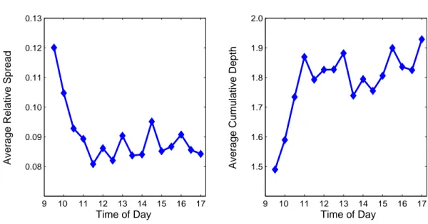
3.3 Time-of-day Effects . . . . 58

5.1 Commonality for Increasing Depth of the Limit Order Book . . . 121

V

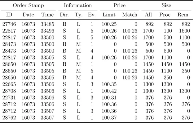
3.1 Example of Allianz’s Trading Protocol . . . . 51

3.2 Summary Statistics of the Data Set – Aggregation . . . . 53

3.3 Average Order Submissions . . . . 56

4.1 Resiliency of Order Book Liquidity . . . . 77

4.2 Resiliency at Different Ticks . . . . 79

4.3 Resiliency at Different Frequencies . . . . 80

4.4 Time Series Impact on Depth Resiliency . . . . 86

4.5 Correlation of Cross-Sectional Factors and Resiliency . . . . 91

4.6 Cross-Sectional Impact on Mean Reversion . . . . 92

4.7 Correlation of Resiliency Measures . . . . 95

5.1 Market Model for Spreads and Depth – Individual Stocks . . . . 107

5.2 Market Model for Spreads and Depth at the Best Limit Prices . . 109

5.3 Market Model for the Extended Depth Measure – Individual Stocks114 5.4 Market Model for Depth at 2.0 % Price Impact . . . 115

5.5 Market Model for the Slope of the Price-Quantity Schedule – In- dividual Stocks . . . 117

5.6 Market Model for the Slope of the Price Impact Function . . . 118

5.7 Market Model for Increasing Depth of the Limit Order Book . . . 120

5.8 PCA Results for the Extended Depth Measures . . . 123

5.9 Impact of the Time of Day . . . 124

5.10 Impact of Market Momemtum . . . 126

6.1 Asset Pricing Inputs . . . 149

6.2 Correlation Structure . . . 150

6.3 Fama-MacBeth Asset Pricing Test . . . 152

VII

6.4 Pooled Asset Pricing Test . . . 153 6.5 Asset Pricing Tests with Different Liquidity Measures . . . 157 A.1 Descriptive Statistics of Spread and Depth Measures at the Best

Limit Prices in the Limit Order Book . . . 172 A.2 Descriptive Statistics for the Depth of the Order Book at 2% Price

Impact and for the Slope of the Order Book . . . 173 A.3 PCA Results for the Spread and the Slope Measures . . . 174 A.4 Impact of the Time of Day: Slope of the Price-Quantity Schedule 174 A.5 Impact of Market Momemtum: Slope of the Price-Quantity Sched-

ule . . . 174

A.6 Relationship between Commonality and Market Return . . . 175

BE Book equity

CAPM Capital Asset Pricing Model CET Central European time DAX Deutscher Aktienindex

ECN Electronic communications network EEX European Energy Exchange

Euribor European Interbank Offered Rate Fibor Frankfurt Interbank Offered Rate

FOK Fill or kill

FSE Frankfurt Stock Exchange

GARCH Generalized Autoregressive Conditional Heteroscedasticity GLS Generalized Least Squares

IOC Immediate or cancel

LR Litzenberger Ramaswamy

LSE London Stock Exchange

MDAX MidCap DAX

ME Market equity

NASDAQ National Association of Securities Dealers Automated Quotations NSC National Security Council

NYSE New York Stock Exchange OLS Ordinary Least Squares PCA Principal component analysis PIN Probability of Informed Trading

SETS Stocks Exchange Trading System (in London) SUR Seemingly unrelated regressions

TecDAX Technology DAX

IX

Symbols in Chapter 2

A, B Ask and bid side subscripts

E Subscript for buy or sell executions (+E, −E) I, P Subscripts for patient and impatient traders

Q

Quantity of limit orders in the book at price l (cumulated) T Time until order execution

U Utility

X True security value

Y Future asset payoff

b Marginal rate of substitution

c Consumption

d Innovation of new information f Index of the patience of traders g Number of spreads in equilibrium h Index of equilibrium spreads

i Firm or stock index

j Index of tick difference between market and limit orders k Number of prices on the ask and bid side (+k, −k) l Index of prices on the ask and bid side (+l, −l)

m Market order volume

n Equilibrium spread

p Price

q Quantity of limit orders with time and price priority

s Bid-ask spread

t Time index

XI

α Price impact of market orders

β Time preference

δ Waiting cost per unit of time

γ Order processing cost

λ Class parameter (for Poisson distribution)

µ Drift component

π Profits

∆

Spread improvement from spread n

to n

Φ Conditioning variables

Θ

Proportion of traders f in the population

Symbols in Chapter 4

A, B Ask and bid side subscripts

AR Order arrival rate

BF Beta Factor

DEP Depth

END End of the trading day IP Informed trader profits L

, L

Stock and market liquidity MC Market capitalization

MO Market order volume

MQ Midprice

nCA Number of cancellations nLO Number of limit orders nMO Number of market orders

OI Order imbalance

P AT Proportion of Patient Traders

SP R Bid-ask spread

T RV Trading volume

UNXV Unexpected volatility

V OL Return volatility

h Conditional volatility

i Firm index

k Index of ticks in the order book (starting at k = 0) l Index of prices in the limit order book (starting at l = 0)

n Number of shares

P Price

r Return

t Time index

α, β, δ, γ Regression coefficients

² Error term

κ Mean reversion parameter

µ Conditional mean of the return ϕ Mean reversion coefficient

∆z Stochastic increment

Θ Long-run mean of liquidity

Symbols in Chapter 5

A, B Ask and bid side subscripts

DEP

Depth at the best bid and ask price L

, L

Stock and market liquidity

M Market subscript

MQ Midprice

P C Principal component

P I Price impact (relative half-spreads)

RS Relative spread

V OL Conditional volatility (squared returns) d Index of the trading day

h Index of the time of day

i Firm index

l Index of prices in the limit order book

n Number of shares

p Price

r Return

t Time index

w Index of rolling ten-day windows x Volume in the limit order book α, β, δ, η, Ψ, ξ Regression coefficients

ε Error term

µ

Time-specific mean

σ

Time-specific standard deviation λ Linear price impact coefficient ρ Quadratic price impact coefficient

Symbols in Chapter 6

BE Book equity

BM Book-to-market factor

C Variance covariance matrix

DEP

Depth at the best bid and ask price DEP

Depth at the k-th tick (cumulated)

HS Half spread

L Liquidity

LLEV Level of liquidity LRES Resiliency factor LSY S Commonality factor M Subscript for the market

ME Market equity

R Excess return

R Monthly return

SIZE Size factor

SP R Bid-ask spread

T Index of test years

V OL Conditional volatility (= squared return)

W Weighting matrix

i Firm index

j Index of pricing coefficients

k Tick index

l Index of prices in the limit order book

p Portfolio index

r

Stock return

r

Risk-free rate of return

r

Market return

s Superscript of stacked vectors and matrices

t Time index

α, β, δ, γ, ξ Regression coefficients β ˆ

Pre-ranking stock beta β ˆ

Portfolio beta

λ Linear price impact coefficient ϕ Mean reversion coefficient

ε Error term

Symbols in the Appendix

C Variance covariance matrix

X Data matrix

Z Standardized X data matrix

i Index of columns in the data matrix j Index of eigenvectors and eigenvalues

x Column in X

z Column in Z

λ Eigenvalue

Λ Diagonal matrix of sorted eigenvalues

γ Eigenvector

Γ Matrix of sorted eigenvectors

Operators and Functions

E Expectation

h(·) Price impact function I(·) Indicator function

int+ Next higher integer value

max Maximum

min Minimum

P r Probability

∆ First difference

σ Standard deviation

Σ Sum

Introduction

The liquidity of a financial security characterizes the speed and ease with which any quantity can be purchased or sold. A liquid asset can be traded quickly and without large price effects. From this point of view, liquidity is desirable for any investor who wishes to buy or sell a security. While liquidity is widely accepted as a component of transaction costs, the risk that arises from illiquidity has re- ceived very little attention in the literature of finance. Most valuation models like the standard CAPM or the Black Scholes option pricing formula even assume frictionless markets with perfectly liquid assets. However, this assumption can be very dangerous. For example, in the 1987 stock market crash and the 1998 bond market failure (see Figure 1.1) liquidity drained from the market dramati- cally, which made it difficult to trade at all. The fall of the Long-Term Capital Management (LTCM) hedge fund, which was strongly exposed to liquidity risk in bond markets, highlights the impact that liquidity risk can have on portfolios.

1

Figure 1.1: Stock and Bond Market Crashes

10−1996 10−1997 10−1998 10−1999 1.0

1.2 1.4 1.6 1.8 2.0 2.2 2.4 2.6 2.8

Panel B

Time Yield Spread (in %)

10−1985 10−1986 10−1987 10−1988 250

300 350 400 450 500

Panel A

Time S&P 100 Total Return Index (in index points)

Figure 1.1 shows the stock and bond market crashes in 1987 and 1998. Panel A plots the value of the S&P100 Total Return Index (in index points) which fell by almost 50% in the autumn of 1987. Panel B plots the yield spread of Moody’s BAA bond index over US government bonds with a constant 10 year maturity (in %). As a result of Russia’s default, the spread increased dramatically.

Against this background I investigate the properties, magnitude and importance of liquidity risk in today’s electronic limit order book markets.

1.1 Key Issues and Relevance

Nowadays all large stock exchanges like New York, London or Frankfurt and all large electronic communication networks (ECNs) such as Island or Instinet are organized as electronic trading facilities. While some trading venues also have market maker features, they all operate on the basis of an open limit order book.

Therefore I focus on an investor’s liquidity risk in the context of electronic limit

order book markets.

To understand the importance of liquidity risk for investors, imagine that an investor who has a stock portfolio suddenly needs to liquidate some positions to meet unexpected cash requirements. If the securities are illiquid at the time, their liquidation will be very costly. Therefore the investor will have to sell more than intended originally to meet his liabilities. This scenario shows that liquidity risk typically constitutes the danger that prices deteriorate heavily in response to trades. In such situations, securities can only be traded at unfavorable prices if at all. Motivated by the demonstrated importance of liquidity risk, I address the following three aspects of liquidity risk in my thesis:

1. How fast does a limit order book refill after liquidity has been taken away?

2. How strongly does liquidity risk spill over across different stocks?

3. To what extent does liquidity risk enter stock prices as a priced factor?

The first question is usually referred to as resiliency. It describes the extent to which new liquidity flows back to the market after the order book has been cleared. The second question addresses the co-movement of liquidity over time, generally referred to as commonality in liquidity. The third question investigates the link between liquidity risk and asset pricing to establish whether liquid assets realize higher prices than their less liquid counterparts. Together, the resiliency, commonality and pricing dimension give a comprehensive picture of liquidity risk in limit order book markets.

To illustrate the economic relevance of liquidity risk, let us have a brief look

at the LTCM case. After a strong decline in liquidity due to the Russian debt cri- sis, LTCM’s portfolio value dropped dramatically (see Figure 1.2). In turn, this triggered off margin calls that had to be met. The fund was forced liquidate large parts of the portfolio in an environment in which it was very expensive to sell off assets. Firstly, the markets for the individual securities were not resilient, which meant that new liquidity did not flow back into the market. The unwinding of large positions was accompanied by strong adverse price movements. Secondly, LTCM found itself amidst a market-wide liquidity crisis. The strong commonality of liquidity prohibited any protection through diversification effects of liquidity risk across instruments. The combination of low resiliency and market-wide illiq- uidity forced LTCM to its knees so strongly that a group of financials institutions led by the Federal Reserve Bank of New York bailed the hedge fund out to avoid complete bankruptcy. The downfall of the LTCM is an acute illustration that investors are well advised to integrate liquidity risk into their risk management.

Before the downfall investors earned well from investing in LTCM which reflects that the market compensates investors for taking on liquidity risk. However, high liquidity risk also implies a higher probability of losses – something that occurred very dramatically in the case of LTCM.

The relevance of liquidity risk at the market-wide level comes from the fact

that liquidity serves as the lifeblood of financial markets. It enables the transla-

tion of information into order flow and prices and thereby promotes the stability

of the trading environment. A sudden drop of liquidity in a certain segment or

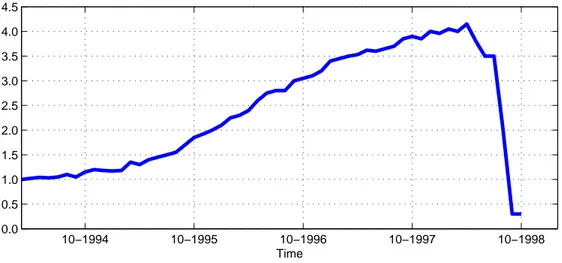
Figure 1.2: Rise and Fall of $1 Invested with LTCM

10−1994 10−1995 10−1996 10−1997 10−1998

0.0 0.5 1.0 1.5 2.0 2.5 3.0 3.5 4.0 4.5

Time

Figure 1.2 shows the gross value of one dollar invested with LTCM from March 1994 to October 1998. LTCM’s funds had a value of $ 4.8 billion in April 1998 of which more than $ 4 billion got wiped out in just a few months because liquidity dried out. The figure follows Lowenstein (2000, p. XV) who gives a detailed account of the rise and fall of the infamous hedge fund.

geographic region can potentially spill over to further segments and countries to

lead market instability on a larger scale. Past crises like in Russia or Indonesia

show that the liquidity of whole regions and markets can dry out and lead to very

destabilizing effects. Therefore, the less resilient and the more systematic liquid-

ity risk is across stocks, the larger the potential for market-wide disruptions. A

deeper understanding of liquidity risk will be very desirable for legislators, regula-

tors, exchanges and financial institutions to enhance the stability and smoothness

of trading in financial markets.

1.2 Contribution to the Literature

The initial interest in the microstructure of security markets and the liquidity of financial assets is often traced back to Demsetz (1968) and Garman (1976).

From then on, the literature has produced an abundance of models of liquidity in security markets. While too numerous to list exhaustively, the most promi- nent approaches include the inventory models of Stoll (1978) and Ho and Stoll (1981), the asymmetric information models of Glosten and Milgrom (1985) and Easely and O’Hara (1987) and the models of strategic trading as in Kyle (1985).

Their theoretical extensions and empirical tests also make up a large body of the liquidity literature. While these approaches address the emergence of liquidity, their extension to liquidity risk – models and tests in which liquidity is stochastic – has only just begun.

The first pillar of liquidity risk that I consider is the resiliency of liquidity.

According to Garbade (1982) a market is resilient if price changes that result

from high order volumes quickly attract new limit orders which, in turn, pull

the price back again. In empirical applications, Holthausen, Leftwich and May-

ers (1987) and Chordia, Roll and Subrahmanyam (2005) study the resiliency of

prices, yet they do not consider liquidity or use liquidity measures, either. Coppe-

jans, Domowitz, Madhavan (2003) and Gomber, Schweickert and Theissen (2004)

analyze the dynamic properties of the limit order book, yet they only focus on the

level of liquidity or half-life measures. Degryse, Jong, Ravenswaaij and Wuyts

(2005) capture resiliency indirectly by the aggressiveness of orders, yet they do not model the refreshment process explicitly. Large (2005) sets up a model of the probability that prices return to pre-trade levels, yet does not distinguish the refreshment process that takes place in the limit order book. In contrast, I extend the literature by directly implementing the Garbade (1982) definition of resiliency. I set up a mean reversion model of liquidity that captures the change in current liquidity in response to past liquidity. Furthermore, I interact the liq- uidity changes with microstructural determinants to examine their impact on the resiliency mechanism of the limit order book.

The second pillar of liquidity risk in my thesis is the stochastic covariation of liquidity across assets. Chordia, Roll and Subrahmanyam (2000) introduced the idea of market-wide liquidity in an empirical study of US quote data. They provide evidence that market liquidity has a significant impact on individual stock liquidity. Brockman and Chung (2002) apply this approach to intraday data from Hong Kong’s order-driven stock market with very similar results. Halka and Huberman (2001) document correlation in the liquidity of different stock portfolios. Hasbrouck and Seppi (2001) on the other hand find little evidence of commonality once deterministic time-of-day effects have been removed. The mixed results and low levels of commonality do not make the current literature very persuasive.

An obvious shortcoming is the confinement to very narrowly

1

The theoretical literature has developed several mechanisms through which the liquidity

supply of different stocks is linked. In these models, the correlation of liquidity preferences, in-

termediary behavior or informational shocks create contagion effects in the liquidity of different

stocks (see Allen and Gale (2000), Kyle and Xiong (2001), Gromb and Vayanos (2002), Fer-

defined measures of liquidity that do not do justice to liquidity risk in limit order markets. Therefore I advance the study of commonality by modeling the liquidity of a limit order book. The section is most closely related to the work of Bauer (2004) and Domowitz, Hansch and Wang (2005). Bauer (2004) performs a principal component analysis of the liquidity in the limit order book across stocks. Domowitz, Hansch and Wang (2005) investigate the influence of order flow and order type correlations on liquidity commonality. The most important difference is that I focus on how commonality in liquidity depends on how deep I look into the limit order book.

The third pillar of liquidity risk that I examine is its impact on expected returns. The first empirical studies examined the relation between the level of liquidity and expected stock returns (see Amihud and Mendelson (1986), Amihud and Mendelson (1989), Eleswarapu (1997), Brennan and Subrahmanyam (1996), Brennan, Chordia and Subrahmanyam (1998) or Amihud (2002)). The next generation of studies focused on the pricing of liquidity risk as opposed to the level alone. They include P´astor and Stambaugh (2003), Gibson and Mougeot (2004) and Acharya and Pedersen (2005). Together these studies provide positive evidence that the level and risk of liquidity get priced. They all consider liquidity movements over long horizons (mostly monthly frequencies). However, liquidity adjustments in limit order book markets are phenomenona that take place and can

nando (2003), Watanabe (2003) and Brunnermeier and Pedersen (2005)). In empirical studies,

Coughenour and Saad (2004) relate commonality in liquidity to common market maker behav-

ior. Domowitz, Hansch and Wang (2005) argue that the correlation of order type choice is the

reason for the correlation of liquidity.

only be observed acurately within hours or even within minutes. Furthermore, most studies do not differentiate between level and risk effects in liquidity. I therefore extend the literature to the pricing effects of liquidity measures that are based on limit order book data. In addition, I separate level and risk effects of liquidity and estimate their impact on returns simultaneously.

In all I bring together the diverse aspects of stochastic liquidity in an attempt to give a comprehensive view of liquidity risk. All of the above issues are applied to limit order book data from a purely quote-driven limit order book market. I use three months of Frankfurt Stock Exchange’s (FSE) electronic protocol which keeps record of all events that took place in their Xetra trading system. With the help of some substantial computer programming that implemented the trading rules of the Xetra system I was able to reconstruct the limit order book from the raw data for any point in time.

As the blue-chip segment of FSE has no additional liquidity supply by specialists and does not face any notable compe- tition from regional exchanges, the order book data enables a clinic view of the liquidity risk of financial securities in electronic limit order book markets.

2

I thank Deutsche Boerse for the electronic trading protocols and initial order book. The

data was supplied and initially prepared in SAS. The subsequent reconstruction programming

took place Gauss. I gratefully acknowledge the support of Helena Beltran-Lopez (Universit´e

Catholique de Louvain), Joachim Grammig and Stefan Frey (Universitaet Tuebingen) who

shared large parts of the programming sequences. The later data construction and econometric

programs were written in Matlab and Eviews. They are disclosed in part in Appendix C and

available upon request.

1.3 Main Results and Procedure

In all, the study of the resiliency of the liquidity supply, the commonality in liquidity and the pricing effects of liquidity risk yield the following results:

• The refill mechanism of the limit order books is strong. The findings suggest that in general resiliency is high. Empty order books are refilled promptly, which restores the normal level of liquidity reasonably fast. Re- siliency is stronger if trading is high, yet if volatility is high, liquidity only increases for investors who wish to buy whereas sales become more difficult.

Informed trading has a weak impact: evidently, liquidity suppliers cannot anticipate the information content of trades in anonymous limit order book markets as they cannot identify the traders behind individual trades.

• The liquidity co-movement in the order book is substantial. Com- prehensive measures of limit order book liquidity as opposed to measures at the best bid and ask price exhibit substantial co-movement: systematic movements across stocks make up about 20% of their overall movement for measures beyond best prices, while the systematic component for measures at the best price is only 2%. These figures underline that market-wide liq- uidity movements are too large to be neglected. Furthermore, commonality is strongly time-varying: while commonality is lower in rising markets, it increases considerably in falling markets.

• Liquidity levels and liquidity risk are priced factors. Both liquidity

levels and liquidity risk get incorporated into stock returns. The higher the level of stock liquidity is, the lower the expected return that an investor will receive from buying that stock. Likewise, the higher the liquidity risk of the stock is, the higher the return paid on the investment. The main implication of these results is that, evidently, investors pay attention to the tradability of stocks.

I proceed as follows: in Chapter 2, I present the basic microstructure theory of securities markets and model the liquidity supply in a limit order book market.

In Chapter 3, I give some details on the market structure, the data that I use in

the empirical sections and some descriptive statistics. In Chapter 4, I examine

the resiliency of the limit order book. Chapter 5 addresses systematic liquidity

risk by focusing on the common movement of liquidity over time. Chapter 6 deals

with the pricing dimension of liquidity levels and liquidity risk. It incorporates

liquidity factors into a Fama-MacBeth framework to study their impact on stock

returns. Chapter 7 concludes.

Liquidity in Limit Order Book Markets

The first section of this chapter gives an overview over the microstructure of financial markets. In the second section I present a static of model of the limit order book, while the third section develops a dynamic model of the limit order book. In the fourth section I conclude how my further empirical research builds on the theoretical literature.

2.1 Market Microstructure

Short-run price dynamics are an important force that drives the liquidity of assets and markets. To understand this process fully, the following section explains price formation on security markets. It shows how short-term price dynamics are embedded in a more long-run valuation process and how short-lived deviations from information efficiency are related to liquidity. Finally I apply these notions to the limit order book.

13

2.1.1 Price Formation with Market Frictions

One of the most prominent fields of modern finance is investment theory. Invest- ment models deal with the equilibrium value of financial assets. They are mostly set in a world in which markets are frictionless and efficient. In such markets, asset prices reflect all available information and thus correspond to their expected true values at any point in time. However, a second implication of frictionless markets is that assets are perfectly liquid. Unfortunately, that is not the case in the real world. This discrepancy is what the literature of market microstructure addresses.

Market microstructure owes its name to Garman (1976) who defines a mar- ket’s microstructure as the interaction of individual exchange actions along time that, in aggregation, make up the market. Loosely speaking, we can think of market microstructure theory as the field that deals with the actual mechanics of financial markets. In particular, it explicitly introduces market frictions. A cen- tral feature is that most microstructure models are characterized by a multitude of prices: agents who offer to trade propose bid prices for sales and ask prices for buys. Market participants who trade against these offers realize so-called trans- action prices. Price data in the media and press usually reports midquotes, the midpoint between the best bid and ask price.

A useful way of distinguishing the investment and microstructure view is by

their time horizons. The investment view considers long-run price dynamics. It

focuses on the asset’s value in the long run which it derives from fundamental

factors about the company. In contrast, the microstructural view considers short- run price dynamics which involve elements of the trading process itself such as the order size, trading activity or market mechanism. In a general sense, mi- crostructural price dynamics are short-run price disturbances around a long-term value process – Hasbrouck (2004) uses the term overlay component.

To illustrate the link between market efficiency and microstructure prices, let us use a slightly more formal representation. Asset pricing theory states that, for a market to be efficient, prices have to be martingales.

The martingale property implies that returns are serially uncorrelated and that prices reflect expectations at all points in time. In a consumption-based asset pricing model, Cochrane (2001) shows how under what conditions prices are martingales. Let c

denote an agent’s consumption in t and let u denote utility from period consumption and let U denote overall utility. An agent’s overall utility then depends on current and future consumption,

U (c

, c

) = u(c

) + β · u(c

), (2.1)

where β is a time preference parameter. If p

denotes an asset’s price, Y

is its future payoff value. The future payoff corresponds to the sum of the price in t + 1 and dividends d, Y

= p

+ d

. If agents maximize utility, the price of the

3

The view of microstructure as a temporary noise component over a more fundamental value process might explain why it is often considered as a second order effect and why microstructure risk was neglected for a long time.

4

A martingale is a stochastic process for which, conditional on today’s information, today’s

price is the best prediction for tomorrow’s price. The random walk model is a popular version

of such a martingale process.

asset is

p

= E

[β u

(c

)

u

(c

) Y

]. (2.2)

An important assumption is that for short time horizons time preference is negligible, β = 1, and there are no dividends, d

= 0. Denoting the marginal rate of substitution as b

:=

, we can under these assumptions set Y

= p

and write the expected future price as

p

= E

[b

p

]. (2.3)

Under the risk-neutral probability measure b

= 1 and E

[p

] = p

. Thus, under a fairly simple set of assumptions, prices in frictionless markets are mar- tingales.

However, when we have several prices (for example for buy and sell orders), the price process is not a martingale any longer. Hasbrouck (2004) shows that for bid and ask prices, Equation 2.3 becomes

p

≤ E

[b

Y

] ≤ p

(2.4)

and that the bid-ask spread prevents returns from being serially uncorrelated. In other words, prices are not equal to expectations at all points in time and, sub- sequently, the market is not informationally efficient. Roll (1984), Stoll (1989), George, Kaul, Nimalendran (1991), Huang and Stoll (1997) and Madhavan and Sofianos (1997) present empirical evidence for short-run return predictability that

5

A large part of the central predictions of asset pricing theory about risk-neutral valuation

goes back to the work of Ross (1976) and Ross (1978). Harrison and Kreps (1979) extended

this to a more formalized theory embedded in a martingale grounding.

arises from microstructure phenomena. This result seems to imply that differing bid and ask prices lead to return predictability and therefore are not consistent with the notion of market efficiency which requires that prices are not predictable.

However, most models in the microstructure literature reconcile market efficiency and microstructural frictions by including an unobservable true value of an asset.

Market participants do not observe the true value, but they receive signals Φ

which they use to form expectations of the true value, E

[Y

|Φ

]. These expec- tations are martingales again. Short-run prices can deviate from expectations, but in the long run expectations ensure that prices are efficient.

The decomposition of microstructure prices into information efficient and non- efficient components leads to another important concept of the microstructure studies: liquidity. The fact that expected values and actual transaction prices need not be the same means that some traders pay more or receive less than the asset is really worth. These costs can vary from stock to stock. Liquidity summarizes differences in prices of the same asset that arise from short-run di- vergences of transaction prices from the expected true value of the asset. In very general terms, assets are considered liquid if reasonable quantities can be traded at prices p

and p

that are not too far from the true value, Y

. However, as O’Hara (1995) and many others point out, this is a very blurry concept. What is a reasonable quantity? When is a price too far from the true value?

While the above models of price dynamics and liquidity serve as a good frame-

work, the actual price process, asset liquidity and subsequent trading costs de-

pend on further issues such as the institutional environment of trading. The most common trading mechanisms nowadays are auction markets. Since the introduc- tion of electronic trading platforms, traders are able to trade continuously when the exchange is open. This is a so-called continuous double auction system. It can be either quote-driven – a market maker supplies liquidity – or order-driven – limit order traders are the only source of liquidity. In practice, markets will often have hybrid structures which combine different elements and systems.

2.1.2 Elements of a Limit Order Book Market

In practice, nearly all markets operate on the basis of an electronic limit order book. Most markets have some distinct features with regard to priority of order execution, competition or transparency. For example, NYSE operates a hybrid system of a limit order book combined with specialists. Paris Bourse and LSE only disclose a fixed number of orders in the book. FSE on the other hand displays each single price in the order book and has no market makers. However, all limit order markets share a set of basic construction elements and rules. Firstly, they all build on the archetypical order forms of limit and markets orders:

• Market orders carry no price limit and are executed immediately against orders in the order book. In the rare case that the book is not liquid enough, they are executed partially and the remaining order lot is executed at the next possible point in time.

• Limit orders carry a pre-specified limit for execution. They are added to

the limit order book and are executed against new incoming market orders as soon as possible. If they are larger than the market order, they are executed partially and the non-executed lot remains in the book.

The most important difference is that market orders have execution certainty, while the execution of limit orders is uncertain. Handa and Schwartz (1996) point out that submitting a limit order has similarities with an option. For example, an investor who places a buy order writes a free put option to the market. Let us assume that the investor places a buy limit order at 100 Euros. If the share price falls below 100 Euros, any trader in the market can hit the limit order at 100 Euros and the option will be executed. This implies that the writer of the option buys the stock above the market price. The lower the market price is, the higher are the losses that result from the limit order. On the other hand, if the market price rises, no trader will execute against the limit order because the stock can be sold at a higher price. Therefore, the profits from the limit order are zero if the stock price rises above 100 Euros. In all, the payoff is negative if the market price falls below the limit price and zero if the market price rises above the limit price. This payoff is identical to a put option. As market participants decide whether to execute against the option, limit order placement is equivalent to a short position in the put. By the same analogy, an investor who places a sell limit order writes a free call option to the market.

The option characteristic of limit orders shows that limit orders supply liq-

uidity by enabling market participants to buy or sell at the prices in the order

book. Limit order traders take over the role that the market maker has in a dealer market. However, some important differences remain between the monop- olistic market maker model and a limit order market: firstly, limit order traders compete amongst each other for the supply of profitable liquidity. Secondly, they know neither the size of incoming market orders nor the identity of the trader.

Therefore, limit order traders have less power to infer the information content of trades than a market maker has in dealer market where he alone sets the quotes.

The differences between market maker quotes and limit orders have implica-

tions for the objectives with which limit orders are used. Traditionally, liquidity

supply only takes place through dealer quotes who make profits by quoting higher

sell prices than buy prices. Traders buy or sell securities because they have either

superior information or exogenous cash requirements. In limit order markets, the

use of limit orders is not confined to liquidity suppliers who submit trades on

both sides of the order book to capitalize the spread. For example, a trader who

has no need for immediacy might submit a limit order instead of a market order

to ensure a good price. On the other hand, not every market order requires su-

perior information or cash demands. A liquidity supplier might spot a stale limit

order and pick it off quickly by means of an immediate market order. In other

words, the choice of a liquidity-supplying limit order depends more strongly on

whether the trader can afford uncertainty of execution – in which case a limit

order is more likely – or whether the trader’s strategy requires immediacy – in

which case a limit order is less likely. Consequently, the notion of limit order

traders as liquidity-supplying dealers is not sufficient. In the following section I develop a formal framework of profit-maximizing limit order placement.

2.2 Static Models of the Limit Order Book

An early model of order placement was developed by Ho and Stoll (1983) where dealers compete for the next incoming order to hit their quotes. Glosten (1994) is the seminal paper on the theory of the limit order book market. Rock (1996) and Seppi (1997) extend the model to include discretized prices and a time priority rule for orders with the same limit price. Sand˚ as (2001) and Frey and Grammig (2005) relax some assumptions of the theoretical model and provide empirical evidence. In the following sections I summarize the Sand˚ as (2001) model. I do not extend the theoretical framework. Instead, the aim is to use this model to show why it is profitable to submit limit orders, why limit orders are submitted at different prices and how this leads to an equilibrium limit order book.

2.2.1 Model Assumptions

The market consists of two types of agents: liquidity suppliers and traders. Liq- uidity suppliers submit limit orders to the order book. They are risk-neutral and profit-maximizing. Traders submit market orders that consume liquidity. They trade either because they have private information or because they wish to satisfy liquidity requirements.

The agents trade a risky asset whose true value at time t is denoted by X

.

This fundamental value of the asset is conditional on all publicly available infor- mation. The law of motion is given by

X

= X

+ d

, (2.5)

where d

is a random innovation. The increment d

contains both new information of trades and new non-trade information in t.

Trading occurs over periods indexed by t. In each period, liquidity suppliers can submit new limit orders until no liquidity supplier wishes to supply a new order anymore. Then a trader arrives and submits a market order that consumes some of the liquidity in the order book. Finally, the new true value of the asset is announced and the procedure starts again.

Let the price vector {p

, p

, ..., p

}

denote the ask prices in the order book where a positive index indicates the ask side. It is ordered from the best price, p

, to the k − th best price p

. Let {Q

, Q

, ..., Q

}

denote the volumes that correspond to the prices of the same index. Likewise, {p

, p

, ..., p

}

and {Q

, Q

, ..., Q

}

represent bid side prices and quantities. The incoming market order volume is denoted by m

where positive quantities, m > 0, are buy orders and negative volumes correspond to sell orders, m < 0. Market orders arrive at the ask side and the bid side with equal probability. Their volume is exponentially distributed with parameter λ. The distribution of m is:

f(m) = (

2λ

e

if m > 0 (buy order)

1

2λ

e

if m <= 0 (sell order). (2.6)

Figure 2.1: Density and Probability Function of Market Orders

0 10 20 30

0.01 0.02 0.03 0.04 0.05

Market Order Volume

Density

Panel A

0 10 20 30

0.10 0.20 0.30 0.40 0.50

Market Order Volume

Probability

Panel B

Figure 2.1 shows the density function (Panel A) and probability function (Panel B) of the market order volume specified in Equation 2.6. The figure assumes λ = 5.

Fig. 2.1 illustrates the density and probability function of the market order vol- ume. Furthermore, each order incurs an order processing cost γ that is quantity invariant and equal for buy and sell orders.

2.2.2 Equilibrium Outcome

Limit order traders have no knowledge about the value of the random innovation

d

, yet they know that market order traders might be informed. Market order

volume is informative about the future value of the asset. The relation between

market order quantity and the change in the fundamental value of X is defined

by a non-decreasing price impact function, h(m). Limit order suppliers update

their beliefs about the future value of the asset subsequent to the volume of the

market order:

E[X

|X

, m] = X

+ h(m) (2.7) The specification of h(·) is assumed linear in the size of the incoming market order m. This leads to the following revision of beliefs:

h(m) = αm (2.8)

A market buy order leads to an increase in revised beliefs and a sell order leads to lower expectations of the asset value. All other things being equal, a larger value of α corresponds to stronger price impacts and a higher revision in beliefs.

On the other hand, if α = 0 the price impact function is horizontal. Then beliefs are not revised at all and the expectation of the future value is not influenced by the size of the incoming market order.

Let us turn to the liquidity supplier’s decision problem whether it is profitable to submit a limit order to the order book. If a limit order that has a price of p

is executed, it generates an expected profit that depends on the size of the subsequent market order:

p

− E[X

|X

, m] − γ = p

− X

− αm − γ (2.9)

The above equation shows that the expected profit depends on the size of the market order: large market orders are a signal of private information on the part of the trader and lower the expected profits of limit order suppliers.

Most importantly however, the execution of a newly submitted limit order is

uncertain. Let q denote the cumulative quantity of all limit orders that have price and time priority. Any infinitesimally small new limit order only gets executed if the incoming market order volume is at least as high as q, m ≥ q. Let I(m ≥ q) denote an indicator function that yields I = 1 for order execution and zero otherwise. At the best price level p

, the expected profit of a liquidity supplier conditional on the execution of the limit order is:

E[p

− X − αm − γ | I = 1] = Z

q

(p

− X

− αm − γ)f (m)dm

= Z

q

(p

− X

− αm − γ) 1

2λ e

dm

= −e

(X

+ γ + α(q + λ) − p

) (2.10)

A limit order trader is indifferent to adding another order to the book at p

if the expected profit is zero. Thus, equating the above profit to zero yields the equilibrium quantity Q

:

Q

= max

½ p

− γ − X

α − λ; 0

¾

(2.11)

The zero profit condition can be extended to the quantity that will be offered at the next best price, p

, in the same way. Order execution is now dependent on m ≥ q + Q

which implies

E [p

− X

− αm − γ | I = 1] = Z

Q+1+q

(p

− X

− αm − γ)f (m)dm (2.12)

and yields the following equilibrium quantity Q

:

Q

= max

½ p

− γ − X

α − Q

− λ; 0

¾

(2.13)

Let l be an index of the prices in the order book (with l = 1, 2, ..., k) and let π denote marginal profits for the case that the limit order gets executed (I = 1).

In the general case, we obtain the following marginal profits for the order book:

E[π

] = e

£

(p

− X

) − α(q + Q

+ λ) − γ ¤

(ask) E[π

] = e

£

(p

− X

) − α(q + Q

− λ) + γ ¤

(bid) (2.14)

The corresponding equilibrium quantities are as follows:

Q

= max

½ p

− X

− γ

α − Q

− λ; 0

¾

(ask) Q

= max

½ X

− p

− γ

α − Q

− λ; 0

¾

(bid) (2.15)

The above equations summarize the status of the limit order book when it is in equilibrium and limit order traders have exploited all profit opportunities that yield a positive expected payoff.

2.2.3 Implications

In this section I highlight the intuition of Equation 2.14 and Equation 2.15 by providing a numerical example. Then I discuss the implications that the model has for the later sections of my thesis.

Figure 2.2 compares the price schedule and the expected payoffs to limit orders

Figure 2.2: Order Book Schedule and Profit Opportunities

0 10 20 30

1 2 3 4 5

Panel A

Market Order Volume Tick

0 10 20 30

1 2 3 4 5

Panel C

Market Order Volume Tick

0 10 20 30

0.2 0.4 0.6

Market Order Volume Panel B

Per Unit Profit

0 10 20 30

0.2 0.4 0.6

Market Order Volume Panel D

Per Unit Profit

Figure 2.2 shows the price schedule and profit opportunities of two limit order books. Panel A and B (blue graphs) correspond to an order book that is in equilibrium, while Panel C and D (red graphs) belong to a book with unexploited profit opportunities. The figures are numerical examples of Equation 2.14 and Equation 2.15 computed for X

= 100, α = 0.1, γ = 0 and λ = 5. The y-axis is in ticks where the first tick is the first possible ask price p

> X

.

traders for two different order books. Panel A and B show a limit order book and payoff for the parameter constellation X

= 100, α = 0.1, γ = 0 and λ = 5.

The book is in the equilibrium state implied by the Equations 2.14 and 2.15. In contrast, Panel C and D show the snapshot of a hypothetical limit order book which is not in equilibrium.

The most striking difference between the two order books is that the submitted

limit order quantities of the non-equilibrium order book are smaller. Panels A and C show the cumulative quantity in the book against their respective prices.

In equilibrium, the marginal break-even quantity at the first tick is 5 and at the second tick it is 10. However, the bottom order book offers only 3 shares at the first tick and only 5 shares at the second tick. Subsequently, it is still profitable to offer 2 more shares at the first tick and 5 more at the second tick.

The unexploited profit opportunities are highlighted in Panels B and D. If we compare the two panels we see that the graph in Panel B always falls to zero before it jumps back up again, while the jumps of the graph in Panel D occur for non-zero values. This underlines the fact that in the non-equilibrium book, marginal profits are still positive.

The equilibrium properties of the Sand˚ as (2001) model help us understand why limit order traders submit liquidity to the limit order book. In particular, we can derive implications that we use in the later sections for the empirical study of the limit order book. The model formalizes the following behavior and incentives of limit and market order traders:

1. Profitability of a Limit Order: Liquidity suppliers submit buy limit

orders at prices which are below their expectation of the future price (and

vice versa for sell limit orders). These limit orders get executed against

market orders and generate a profit for limit order traders. This implies

that, ceteris paribus, a higher amount of market order trading offers higher

profit opportunities for liquidity suppliers.

2. Position in the Limit Order Queue: There are profit opportunities along the whole price-quantity schedule of the limit order book. Limit orders near the best tick have higher execution probability and lower con- ditional profits, while limit orders further away have lower execution proba- bility but higher conditional profits. This implies that limit order flows can take place deeper in the book even if there is no change at the best price.

3. Transaction Costs of Market Orders: The equilibrium limit order book shows that large market orders get executed against several different limit order prices. The larger the market order, the larger the marginal costs that it incurs. Large market orders take away depth from the limit order book and shift the price-quantity schedule. This implies that liquidity beyond best prices becomes relevant for large orders.

4. Information Signals: Limit order traders take the size of trades as an informative signal of the true value of the asset which they take into ac- count in their future liquidity supply. They interpret large orders as highly informative and revise their beliefs particularly strongly. This implies that for limit order flows in any period we have to distinguish whether they took place in an information-intensive or low-information environment.

The model implications might only highlight simple mechanics of limit order

book markets, but they are a good starting point to compare the empirical fea-

tures of the limit order book against. Yet before we proceed any further, let us

cast a brief look at the weaknesses of the model. Firstly, when an order book is in equilibrium, the model does not allow the submission of new liquidity at the best prices. New limit orders only replace liquidity at the furthest tick.

A second weakness is that market orders are assumed to be exogenous. In practice, however, the dynamics of the limit order book are far more complex.

2.3 Dynamic Models of the Limit Order Book

In the following section I present a dynamic model of a limit order book market.

The theoretical literature includes models by Parlour (1998), Foucault (1999), Parlour and Seppi (2003)), Goettler, Parlour and Rajan (2004) and Foucault, Kadan and Kandel (2005). I present a simplified version of Foucault, Kadan and Kandel (2005) who endogenize the decision between limit and market order placement.

While the previous model provided implications why limit order traders trade and where they submit their limit orders, I present the following model to obtain hypotheses for the dynamic properties of limit order flow.

6

However, Hasbrouck (2004) points out that this problem is overcome when uncertainty is introduced, albeit at the cost of simple analytic solutions.

7

In contrast, Parlour (1998) models how the order placement decision depends on the depth

of the limit order book at the best quotes. Foucault (1999) addresses the risk that limit order

strategies lose against agents who have better information. Parlour and Seppi (2003) set up a

dynamic model of different exchanges that compete against each other for order flow. Goettler,

Parlour and Rajan (2004) model limit order trading as a stochastic game that takes place

sequentially. I present the Foucault, Kadan and Kandel (2005) framework because it is based

on the immediacy of market orders versus the delayed execution of limit orders. This framework

is well-suited to derive hypotheses for the time series behavior of liquidity flows as I will be

doing in the following sections.

2.3.1 Model Assumptions

The market is organized as a limit order book in which market participants trade one single security. The highest sell price of the security is p

and the lowest buy price is p

(with p

> p

> 0). The best ask price is denoted by p

and the best bid price by p

.

The model investigates the dynamics of the bid- ask spread, s := p

− p

, within the maximum price range, p

− p

. At the endpoints of the price interval traders offer to sell and buy an unlimited amount of shares.

Market participants arrive at the market following a Poisson process with parameter λ > 0. The model has an infinite horizon and the times between trade arrivals are exponentially distributed with an expectation of

. Market participants are risk-neutral. Upon their arrival they submit either a market order, which is executed immediately, or a limit order, which is executed later, but at a better price. Furthermore, each agent bears waiting costs δ (per unit of time) for the time until order execution. Traders either belong to the class of impatient traders or patient traders: impatient traders value fast trade execution and have high waiting costs of δ

, while patient traders have low waiting costs of δ

(with δ

> δ

). The proportion of patient traders to impatient traders in the population is Θ

; the proportion of impatient traders is Θ

= 1 − Θ

.

The trading mechanism of the market is a centralized limit order book in

8

For simplicity I assume a unit tick size. The results are qualitatively identical if a tick size

variable is included, yet they make the model unnecessarily complicated as it is not my aim to

study tick size effects.

which all limit orders are executed according to price priority. To facilitate the analysis of the equilibrium outcome, Foucault, Kadan and Kandel (2005) make the following assumptions:

• Traders arrive only once, submit a market or limit order of size 1 and exit the market. Orders that have been submitted cannot be cancelled or revised.

• Limit orders always improve the current best price and reduce the spread by at least one tick. They cannot queue at the same price.

• A buy order is always followed by a sell order and sell orders are always followed by buy orders. The probability that the first order is a buy is 0.5.

I denote the execution price of buy and sell orders by p

and p

. A buyer either submits a market order for which he pays the lowest ask price, p

, or submits a limit order on the bid side. The limit order enters the order book at a new best bid price, p

. Likewise, a seller either trades at the best bid price or enters a new best ask price. Hence, execution prices can be written as

p

= p

− j (2.16)

p

= p

+ j (2.17)

where j denotes the number of ticks from the best price in the limit order book

against which the order could be executed (with j ∈ {0, ..., s − 1}). For a market

order j = 0, the time to execution is zero and therefore the waiting costs are zero,