Traveling Solitary Waves in the Periodic Nonlinear Schrödinger Equation with Finite Band Potentials

Periodic Nonlinear Schr¨ odinger Equation with Finite Band

Potentials

Tom´ aˇs Dohnal

Preprint 2013-05 Mai 2013

Fakult¨ at f¨ ur Mathematik

Technische Universit¨ at Dortmund Vogelpothsweg 87

44227 Dortmund tu-dortmund.de/MathPreprints

SCHR ¨ODINGER EQUATION WITH FINITE BAND POTENTIALS

Tom´aˇs Dohnal ^∗

Abstract. The paper studies asymptotics of moving gap solitons in nonlinear periodic structures of finite contrast (“deep grating”) within the one dimensional periodic nonlinear Schr¨odinger equation (PNLS). Periodic structures described by a finite band potential feature transversal crossings of band functions in the linear band structure and a periodic perturbation of the potential yields new small gaps. An approximation of gap solitons in such a gap is given by slowly varying envelopes which satisfy a system of generalized Coupled Mode Equations (gCME) and by Bloch waves at the crossing point. The eigenspace at the crossing point is two dimensional and it is necessary to select Bloch waves belonging to the two band functions. This is achieved by an optimization algorithm. Traveling solitary wave solutions of the gCME then result in nearly solitary wave solutions of PNLS moving at anO(1) velocity across the periodic structure. A number of numerical tests are performed to confirm the asymptotics.

Key words. moving gap soliton, periodic structure with finite contrast, finite band poten- tial, nonlinear Schr¨odinger equation, Gross-Pitaevskii equation, coupled mode equations, envelope approximation, Lam´e’s equation

AMS subject classifications. 35Q55, 35C20, 37L60, 33E05, 41A60

1. Introduction. Coherent pulses traveling across nonlinear periodic structures like, e.g., optical pulses in photonic crystals, are of interest from a phenomenological as well as applied point of view. A special case of pulses in periodic structures are gap solitons, which are localized coherent waves with their frequency (or propagation constant) inside a spectral gap of the corresponding linear spatial spectral problem.

In certain cases gap solitons exist in families parametrized by velocity so that tuning of the velocity at one fixed frequency becomes possible.

In the vicinity of spectral edges gap solitons can be approximated by asymptotic slowly varying envelope approximations. The approximation consists of slowly varying envelopes multiplying Bloch waves belonging to the spectral edge.

In periodic structures with afinite (rather than infinitesimal)contrast a spectral edge is defined by one or more extrema of the band structure so that the correspond- ing Bloch waves have zero group velocity. Finite contrast structures are sometimes referred to as “deep grating” structures [5]. The scaling of the envelopes in the generic case of locally parabolic band structure extrema is

√εA(√ εx, εt),

where 1 ≫ε > 0 is the asymptotic parameter, see [4] and Sec. 2.4.1 of [14] for 1D examples and [7, 8] for 2D examples including rigorous justification of the asymp- totics. The authors of [4] consider the 1D nonlinear wave equation with periodic coefficients while in Sec. 2.4.1 of [14] and in [7,8] the periodic nonlinear Schr¨odinger equation is studied. The scaling of the envelopes and the linear part of the effective equations for the envelopes are, however, determined only by the local shape of the band structure. In both cases the effective equations are either scalar or coupled cubically nonlinear Schr¨odinger equations in the variables (X, T) := (√εx, εt) with constant coefficients. Localized solitary wave solutions of the effective equations with

∗Technische Universit¨at Dortmund, Fakult¨at f¨ur Mathematik, Vogelpothsweg 87, D-44227 Dort- mund, Germany; Email: tomas.dohnal@math.tu-dortmund.de; Date: May 15, 2013

1

velocity v in the (X, T)-variables produce gap soliton approximations with only the infinitesimal velocity√εv in the original (x, t)-variables due to the slower scaling of time than space. The approximation is valid on time intervals of lengthO(ε⁻¹).

Insmall (infinitesimal)contrast structures the asymptotic situation for gap soli- tons is, however, different. Note that periodicity with infinitesimal contrast (here denoted by ε) can open spectral gaps only in 1D problems due to the overlapping of band functions in higher dimensions. In 1D infinitesimal structures gaps open from points where band functions intersect in a transversal manner so that the Fourier waves at ε = 0 at the intersection points have nonzero group velocity±cg. These Fourier waves then play the role of carrier waves in the asymptotics for gap solitons.

The nonzero group velocity also results in equal scaling of time and space in the corresponding envelopesA1,2, namely

√εA1,2(εx, εt),

and the effective model for the envelopes A1,2(X, T), where (X, T) := (εx, εt), is a system of two first order equations, so called Coupled Mode Equations (CMEs)

i(∂TA1+cgA1) +κA2+α(|A1|²+ 2|A2|²)A1= 0

i(∂TA2−cgA2) +κA1+α(|A2|²+ 2|A1|²)A2= 0 (1.1) withκ, α∈R. The derivation and justification of (1.1) for the case of a 1D nonlinear wave equation is in [18, 10] and for the 1D periodic nonlinear Schr¨odinger equation in [15]. Choosing a moving solitary wave solution [3] of (1.1), the resulting gap soliton approximations haveO(1) velocity due to the equal scaling of time and space in A1,2(εx, εt). The approximation is, once again, valid on time intervals of length O(ε⁻¹).

Besides the above asymptotic approximations on long but finite time intervals one can also seek exact moving solitary waves. Moving breathers have been considered in [16] for the 1D periodic nonlinear Schr¨odinger equation with a small contrast. The resulting breathers travel at anO(1) velocity but could be shown to be localized only on large but finite spatial intervals.

In this paper we consider the asymptoptics on large but finite time intervals and show that an analogous asymptotic situation to that of the infinitesimal contrast can arise also in 1D structures with finite contrast. As we explain, periodic perturbations of so called finite band potentials are a suitable example. Such perturbations lead to the opening of gaps from transversal crossings of band functions. In these gaps one can approximate gap solitons via a slowly varying envelope ansatz. The effective equations are shown to be a generalization of the classical CMEs (1.1) from the infinitesimal contrast case. Families of localized solutions parametrized by velocity can be constructed by a homotopy continuation from explicitly known solutions of (1.1).

The resulting gap soliton approximations travel at a wide range of O(1)-velocities across a periodic structure of finite contrast. The analysis is performed for the 1D Gross-Pitaevskii equation / periodic nonlinear Schr¨odinger equation (PNLS)

i∂tu+∂_x²u−V(x)u−σ|u|²u= 0, (1.2) whereσ∈Rand

V(x) =VFB(x) +εW(x)

with a (real) finite band potential VFB of periodd > 0 and a piecewise continuous reald-periodic perturbation W. Nevertheless, the analysis carries over, for example, to the nonlinear wave equation ∂_t²u−∂²_xu+V(x)u+σu³ = 0 with u real without significant modifications.

A difficulty in setting up the asymptotic ansatz is the selection of Bloch waves with the right group velocity at a crossing point of band functions. This is equiv- alent to constructing Bloch wave families smooth in k across the crossing points.

The eigenspace at the crossing points is two dimensional and we propose a simple optimization algorithm for selecting the right linear combination of a given basis.

The rest of the paper is structured as follows. In Sec. 2 the linear spectral problem (−∂_x²+V(x))ψ=λψ corresponding to the PNLS is reviewed including the relevant results of Bloch theory. An example of a finite band potential and its band structure is then given. In Sec. 3 the problem of selecting Bloch waves smooth in k is discussed and an optimization algorithm for this selection is introduced. Sec.

4 provides a formal asymptotic analysis of gap solitons and the derivation of the generalized CMEs as effective equations for the slowly varying envelopes. In Sec. 5 solutions of the generalized CMEs are constructed via homotopy from solutions of CMEs. Finally, in Sec. 6 numerical tests verify the expected convergence of the asymptotic approximation error with respect toεon time scales ofO(ε⁻¹).

2. Review of Bloch waves and finite band potentials.

2.1. Spectral Problem. The linear spectral problem corresponding to (1.2) is

Lψ=λψ, (2.1)

where L:=−∂_x²+V(x). The spectrum ofL is purely continuous (Theorem XIII.90 in [17]) and consists of intervals (bands) possibly separated by gaps. In detail

σ(L) = [

n∈N

[s2n−1, s2n],

where sn∈Rand s2n−1 < s2n ≤s2n+1, N:={1,2,3, . . .}. The spectrum as well as the corresponding solutionsψcan be determined from the Floquet-Bloch problem for the Hill’s equation (2.1). Texts on Floquet-Bloch theory for the Hill’s equation with periodic coefficients include [12,9, 17]. The Floquet-Bloch problem is the eigenvalue problem

Lψ(x, k) =ω(k)ψ(x, k), x∈[0, d)

ψ(d, k) =e^ikdψ(0, k) (2.2)

with k ∈ (−π/d, π/d]. For each k ∈ (−π/d, π/d] problem (2.2) has a countable set of eigenvalues (ωn(k))n∈N. We number the eigenvalues according to size. The family ωn : k 7→ ωn(k),n ∈ N is usually referred to as the band structure and we call the individual ωn(k) the band functions. The quasi-periodic solutions ψn(x, k) corresponding toωn(k) are called Bloch waves and have the form

ψn(x, k) =pn(x, k)e^ikx, pn(x+d, k) =pn(x, k). (2.3) We normalize kψn(·, k)k^L2(0,2d) = 1. Note that due to the form (2.3) we have kψn(·, k)k²L²(0,d)= 1/2. The spectrum ofL can be determined via

σ(L) = [

n∈N k∈(−π/d,π/d]

ωn(k).

Complex conjugation of (2.2) produces the symmetry

ωn(−k) =ωn(k) (2.4)

for allk∈(−π/d, π/d), and for simple eigenvaluesωn(k) we also have

ψn(x,−k) =ψn(x, k). (2.5)

As a second order equation, (2.1) has only two linearly independent solutions. The even symmetry ofωn(k) thus implies that double eigenvaluesωn(k) can occur only at k=k0∈ {0, π/d}. This multiplicity happens if two band functionsωn(k) andωn+1(k) touch. For a touching point atk0= 0 there are two linearly independentd−periodic Bloch functions and for k0 = π/d there are two linearly independent 2d−periodic Bloch functions, cf. Theorem 2.1 in [12].

2.2. Finite Band Potentials. As mentioned in the introduction, we wish to study potentials V given by periodic perturbations of finite band potentials. A clas- sical example of a finite band potential is

VFB(x;m, η) =m(m+ 1)η sn²(x;η), (2.6) where sn is the Jacobi elliptic function, m ∈R and η ∈(0,1). Equation (2.1) with V = VFB is ussually called Lam´e’s equation. The function sn is odd and has the period 2R1

0

√_(1−t2dt)(1−ηt²). Therefore, the period ofVFB(·;m, η) is d=

Z 1

0

dt

p(1−t²)(1−ηt²).

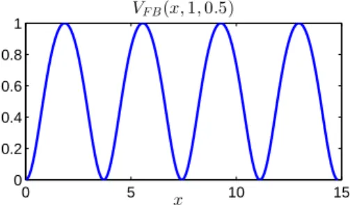
It is known that Lam´e’s equation has exactly m finite spectral gaps (plus the semi- infinite gap (−∞, s1)) if and only ifm∈N, see [13]. In our computations we choose m= 1 and η= 1/2. Forη = 1/2 an approximate value of the period is

d≈3.708149365

as provided by [2]. In Fig. 2.1 the function VFB(x; 1,1/2) is plotted. Note that all

0 5 10 15

0 0.2 0.4 0.6 0.8 1

x VF B(x,1,0.5)

Fig. 2.1. The finite band potentialV_FB(x; 1,1/2).

finite band potentials are analytic, cf. Theorem XIII.91 (d) in [17].

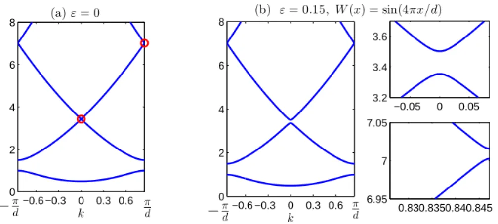
The band structure of (2.2) for V(x) = VFB(x; 1,1/2) is shown in Fig. 2.2 (a), where the sole spectral gap is clearly visible. As the numerical results suggest, under the periodic perturbation εsin(4πx/d) new gaps open from the first two touching points of band functions. These points are circled in Fig. 2.2(a) and the new gaps bifurcating from them forε >0 are magnified in (b). In these computations problem (2.2) was discretized via the fourth order centered finite difference scheme withdx= d/1200.

−0.6 −0.3 0 0.3 0.6 0

2 4 6 8

k (a)ε= 0

−

π d

π

d ^{−0.6 −0.3 0 0.3 0.6}

0 2 4 6 8

k

(b) ε= 0.15, W(x) = sin(4πx/d)

−

π d

π d

−0.05 0 0.05 3.2

3.4 3.6

0.830.8350.840.845 6.95

7 7.05

Fig. 2.2. The band structure of (2.2)for V(x) =V_FB(x; 1,1/2) +εsin(4πx/d) with (a) ε= 0 and (b)ε= 0.15. In (a) gap bifurcation points are circled. In (b) two regions where gap opening occurs are magnified.

3. Smoothness of Bloch Waves in k. For the asymptotics of gap solitons in gaps bifurcated from touching points of band functions we need to be able to define the group velocity at these points and to find a Bloch wave with this group velocity. The group velocity requires at least differentiability of the band functions. By standard eigenvalue perturbation theory [11] eigenvalues ωn(k) are analytic in k in regions where they are simple, i.e. away from touching points k0. Clearly, ωn(k), which are numbered according to size, are generally not differentiable at touching points, see e.g. ω2(k) and ω3(k) in Fig. 3.1 (a), which is the exampleV =VFB(x,1,1/2).

As shown after Theorem XIII.89 of [17], for the 1D problem (2.2) with a piecewise continuous V(x) a relabeling is possible so that the resulting band functions are analytic everywhere. For a given touching point (k, ω) = (k0, ω0) we denote these analytic functions ω+(k) and ω−(k), where ±ω±^′ (k) ≥ 0. For the touching point k0= 0, ω0≈3.428 of the above example the functions ω±(k) are plotted in Fig. 3.1 (b). For a touching point withk0=π/dthe derivatives ofω±(k) atk=k0are defined after the 2π/d-periodic extension ofω±(k).

The Bloch wavesψ+(x, k) corresponding toω+(k) have nonnegative group veloc- ity and due to symmetry (2.4) the Bloch wavesψ−(x, k) corresponding toω−(k) have the opposite group velocity, i.e.

ω^′₊(k) =−ω^′−(−k) for allk∈(−π/d, π/d). (3.1) Note that the derivatives ofω±(k) can be expressed as an integral of Bloch waves:

ω^′±(k) =−2i Z 2d

0

∂xψ±(x, k)ψ±(x, k)dx (3.2) as follows by the differentiation ofLψ±(x, k) =ω±(k)ψ±(x, k) in k. Symmetry (2.5) translates to

ψ+(x, k) =ψ−(x,−k) for allk∈(−π/d, π/d)\ {k0}. (3.3) For our gap soliton asymptotics we need to determine the Bloch wavesψ±(x, k0), which will play the role of carrier waves. In general it is unknown whether Bloch waves

−0.6 −0.3 0 0.3 0.6 0

1 2 3 4 5 6 7 8

−

π d (a)

ω₂ ω2

ω1

ω₃ ω₃

−0.6 −0.3 0 0.3 0.6 0

1 2 3 4 5 6 7 8

−

π d (b)

ω1

ω₊

ω+

ω₋ ω₋

Fig. 3.1. Band structure of (2.2) for V(x) = VFB(x; 1,1/2) with eigenvalues labeled according to size in (a) and according tok−smoothness in (b).

can be chosen smooth with respect to k throughout touching points. In Theorem XIII.89 of [17] it is shown that for piecewise continuousV(x) continuity with respect tokcan be achieved at the touching points. It seems that literature offers no stronger regularity results. For the purposes of our gap soliton asymptotics, we propose the following algorithm to selectψ±(x, k0).

3.1. Choice of the Carrier Waves ψ±(x, k0). At the intersection of the band functions ω±(k) at (k, ω) = (k0, ω0) there are two linearly independent solutions v1

and v2 of (2.2) with the (quasi-)periodic extension of v1 being even and that of v2

being odd inx[9]. Ask0∈ {0, π/d}, the solutions are 2d−periodic and can be chosen real. We normalizekv1,2k^L2(0,2d)= 1.

The Bloch waves φ1(x) :=ψ+(x, k0) and φ2(x) :=ψ−(x, k0) are specific linear combinations ofv1 andv2. We write

φ1=av1+bv2, φ2=cv1+dv2. (3.4) Due to the continuity in k symmetry (3.3) has to hold also atk =k0, i.e. we have φ2=φ1 so that

c= ¯a, d= ¯b

and onlya, b∈Cneed to be determined. We define (a, b) as the solution of

δlim→0kψ+(·, k0−δ)−(av1+bv2)kL²(0,d)= 0.

For the purposes of the numerical implementation we fix a small δ > 0 (typically δ= _2d^π10⁻³) and minimize

J(a, b) :=kψ^δ₊−(av1+bv2)k²L²(0,d),

where ψ^δ₊(x) :=ψ+(x, k0−δ). This is a four dimensional optimization problem (in the real and imaginary parts ofa andb) but it can be reduced to an effectively one dimensional problem via the following two constraints.

Firstly, we require orthogonality ofφ1 andφ2. 0 =

Z 2d

0

φ1φ2dx= Z 2d

0

φ²₁dx= Z 2d

0

(av1+bv2)²dx=a²+b²,

where the second equality follows from φ2 =φ1 and the last equality from the nor- malization ofv1andv2and their opposite spatial symmetry such thatv1v2is an odd function acrossx=d. Consequently result we have

b=sia with s∈ {−1,1}, (3.5)

and it remains to determinea∈Cands∈ {−1,1}.

Secondly, we use the normalization constraintkφ1kL²(0,2d)= 1 so that 1 =kφ1k²L²(0,2d)=

Z 2d

0

(av1+siav2)(¯av1−si¯av2)dx

=|a|² Z 2d

0

(v²₁+v₂²)dx= 2|a|² and

a= 1

√2e^iρ, ρ∈R.

As a result we need to minimize with respectρ∈Rands∈ {−1,1} the function J˜(ρ, s) :=kψ₊^δ − 1

√2e^iρ(v1+siv2)k²L²(0,d)

= Z d

0

1

2(v₁²+v²₂) +|ψ₊^δ|²−√

2Re(ψ₊^δe^−iρ(v1−siv2))dx

=1−√

2Re(ψ₊^δe^−iρ(v1−siv2))dx

=1−√ 2

"

cos(ρ) Z d

0

Re(ψ₊^δ(v1−siv2))dx+ sin(ρ) Z d

0

Im(ψ^δ₊(v1−siv2))dx

# ,

where in the one but last equality the normalization of v1,2 as well as the property kψ₊^δk²L²(0,d)= 1/2, cf. Sec. 2.1, have been used. The derivative of ˜J with respect to ρvanishes at those valuesρ=ρ∗, for which

tan(ρ∗) = Rd

0 Im(ψ₊^δ(v1−siv2))dx Rd

0 Re(ψ₊^δ(v1−siv2))dx.

The choice of the optimals∈ {−1,1} can be done by simply comparing ˜J(ρ∗, s) for the two values of s. Indeed, the numerics show that one choice of sleads to a near zero value of ˜J while the other choice leads to a value close to 1.

For purposes of the asymptotics in Sec. 4 we multiply the familiesψ+ and ψ−

(includingφ1 andφ2) by complex phase factors to ensure Z 2d

0

W(x)φ1φ2dx∈R, (3.6)

cf. the coefficientκin (4.3). The phase factors can be determined explicitly. Forφ1,2

as defined in (3.4) we have Z 2d

0

W(x)φ1φ2dx= Z 2d

0

W(x)φ²₁dx= Z 2d

0

W(x)(a²v²₁+b²v²₂+ 2abv1v2)

= 2ab Z 2d

0

W(x)v1v2dx= 2sia² Z 2d

0

W(x)v1v2dx, due tob=siaandR2d

0 W(x)v²₁dx=R2d

0 W(x)v₂²dx. Definingϕ:= arg sia²R2d

0 W(x) v1v2dx), we, therefore, set

ψ˜+(x, k) :=e^−iϕ/2ψ+(x, k), ψ˜−(x, k) :=e^iϕ/2ψ−(x, k), φ˜1(x) :=e^−iϕ/2φ1(x), φ˜2(x) :=e^iϕ/2φ2(x)

and drop the tildes, so that now (3.6) holds. Note that the orthogonality, conjugation symmetry and normalization ofφ1andφ2 are preserved under the phase shift.

In order to test the algorithm of constructingφ1=ψ+(x, k0) andφ2=ψ−(x, k0), we compare the value

cg:=ω₊^′ (k0) =−2i Z 2d

0

∂xφ1(x)φ1(x)dx (3.7) as given by (3.2) with a finite difference approximation c^FD_g of ω₊^′ (k0) computed using the fourth order centered finite difference formula with dk = _5∗^π₂nd for n = 0,1,2, . . . ,6. The integral in cg was approximated using the trapezoidal rule with dx=d/1200. Fig. 3.2shows a clear convergence ofc^FD_g tocg asdkdecreases.

10⁻² 10⁻¹

10⁻⁸ 10⁻⁶ 10⁻⁴

dk

|cg−c^{F D}_g |

Fig. 3.2.Convergence ofc^FDg tocg in (3.7)with respect to thek-discretization parameter dk.

4. Asymptotics of gap solitons in narrow gaps. A genericd−periodic per- turbationεW of ad−periodic finite band potentialVFB in

V =VFB+εW

generates forε >0 infinitely many gaps in the spectrumσ(−∂_x²+V), see Theorem 4.6.1 in [9]. Let us assume that one such new gap opens. As explained in Sec. 2, the opening occurs at the intersection of spectral bandsω+(k) andω−(k) at k=k0∈ {0, π/d}.

Letφ1 andφ2 be the Bloch waves constructed in Sec. 3.1. They are 2d−periodic and normalized to satisfykφ1,2k^L2(0,2d)= 1.

Analogously to [5] we propose now the following slowly varying envelope ansatz for gap solitons in the new infinitesimally small spectral gap

u(x, t)∼ε^1/2

2

X

j=1

Aj(X, T)φj(x)e^−iω0t+ε^3/2u1(x, X, T)e^−iω0t (4.1) X:=εx, T :=εt

for ε→ 0 with u1 being 2d−periodic in x. Note that the ansatz (4.1) is analogous to the case of gap solitons in periodic structures with infinitesimally small contrast, where the carrier Bloch wavesφ1,2are replaced by plane waves [10,18]. Substituting (4.1) in (1.2) and collecting equal powers ofεproduces atO(√ε) the linear problems

(L−ω0)φ1= 0, and (L−ω0)φ2= 0, which are satisfied by the definition ofφ1,2.

AtO(ε^3/2) we obtain

(L−ω0)u1= (iφ1∂T+ 2∂xφ1∂X)A1+ (iφ2∂T + 2∂xφ2∂X)A2 (4.2)

−W(x) (A1φ1+A2φ2)−σ |A1|²A1|φ1|²φ1+|A2|²A2|φ2|²φ2

+2|A1|²A2|φ1|²φ2+ 2|A2|²A1|φ2|²φ1+A²₁A2φ²₁φ2+A²₂A1φ²₂φ1 .

By Fredholm alternative a 2d−periodic solution (with respect to x) of (4.2) exists only if the right hand side is L²(0,2d)−orthogonal toφ1 and φ2. The resulting two solvability conditions are thegeneralized Coupled Mode Equations (gCMEs)

i (∂T +cg∂X)A1+κA2+κsA1+α(|A1|²+ 2|A2|²)A1

+β(2|A1|²+|A2|²)A2+βA²₁A2+γA²₂A1= 0, i (∂T −cg∂X)A2+κA1+κsA2+α(|A2|²+ 2|A1|²)A2

+β(2|A2|²+|A1|²)A1+βA²₂A1+γA²₁A2= 0,

(4.3)

where

cg=ω^′₊(k0) =−2i Z 2d

0

φ^′₁(x)φ1(x)dx= 2i Z 2d

0

φ^′₂(x)φ2(x)dx∈R, κ=−

Z 2d

0

W(x)φ2φ1dx=− Z 2d

0

W(x)φ1φ2dx∈R, κs=−

Z 2d

0

W(x)|φ1|²dx=− Z 2d

0

W(x)|φ2|²dx∈R, α=−σ

Z 2d

0 |φ1|⁴dx=−σ Z 2d

0 |φ2|⁴dx=−σ Z 2d

0 |φ1|²|φ2|²dx∈R, β =−σ

Z 2d

0 |φ1|²φ2φ1dx=−σ Z 2d

0 |φ2|²φ2φ1dx∈C, γ=−σ

Z 2d

0

φ²₂φ1

2dx∈C.

The identities incg, α, κsandβfollow fromφ2=φ1. The fact thatκ∈Rfollows from (3.6) andcg∈Rcan be seen via integration by parts. In fact, our choicecg=ω₊^′ (k0) ensurescg>0.

Remark 4.1. A system of the same type as (4.3) appears in [5] but no explanation of which periodic structures lead to this effective model is given.

Remark 4.2. Note that for odd functions W, i.e. W(x) =−W(−x) for all x∈R, we getκs= 0 due to the following calculation.

Z 2d

0

W(x)|φ1|²dx= Z 2d

0

W(x)(|a|²v₁²+|b|²v₂²)dx+ Z 2d

0

W(x)(ab+ba)v1v2dx The first integral on the right hand side is zero due to the evenness ofv²₁ andv₂²about x=d and the second integral vanishes due to(3.5).

In fact, one can assume without loss of generality that κs= 0because the terms κsA±can be removed by the simple gauge transformationA±(X, T)→A±(X, T)e^iκsT. Remark 4.3. The above formal asymptotics predict that the correction term u1 is a sum of terms of the form B(εx, εt)f(x), where B is any of the (X, T)-dependent coefficients on the right hand side of (4.2), i.e. ∂TA1, ∂XA1, A2, A1,|A1|²A1 etc.

Therefore, assuming boundedness ofA1,2 and its first derivatives, we formally get kε^3/2u1(·, ε·, T)k^L2(R)=O(ε). (4.4) 5. Construction of Solutions to the Generalized Coupled Mode Equa- tions. Explicit solutions of (4.3) are not known. System (4.3) is, however, a gen- eralization of the classical CMEs (1.1) for envelopes of pulses in the nonlinear wave equation with a periodic structure of infinitesimal contrast [3, 10]. gCMEs (4.3) re- duce to (1.1) if we set κs = β = γ = 0. System (1.1) has the following explicitly known family of solitary waves, see [3,10,6],

A⁽⁰⁾₁ =νae^iη s |κ|

2|α|sin(δ)∆⁻¹e^iνζsech(θ−iνδ/2), A⁽⁰⁾₂ =−ae^iη

s |κ|

2|α|sin(δ)∆e^iνζsech(θ+ iνδ/2),

(5.1)

where

ν= sign(κα), a=

r2(1−v²)

3−v² , ∆ = 1−v

1 +v 1/4

, e^iη =

−e^2θ+e^−iνδ e^2θ+e^iνδ

2v 3−v2

θ=µκsin(δ) X

cg −vT

, ζ=µκcos(δ) v

cg

X−T

, µ= (1−v²)^−1/2 with the parameters of velocityv∈(−1,1) and “detuning”δ∈[0, π].

For δ =π/2 we get ζ = 0 and both A⁽⁰⁾₁ and A⁽⁰⁾₂ depend only on the moving frame variable ˜θ=θ(δ=π/2) =µκ

X cg −vT

. For this case we carry out a numerical homotopy continuation of solutions (5.1) to solutions of (4.3) withκs, βandγnonzero.

In the moving frame variable ˜θsystem (4.3) reads

ia+∂θ˜A1+κA2+κsA1+α(|A1|²+ 2|A2|²)A1

+β(2|A1|²+|A2|²)A2+βA²₁A2+γA²₂A1= 0, ia−∂θ˜A2+κA1+κsA2+α(|A2|²+ 2|A1|²)A2

+β(2|A2|²+|A1|²)A1+βA²₂A1+γA²₁A2= 0,

(5.2)

wherea+=µκ(1−v) anda−=−µκ(1 +v).

We solve (5.2) numerically in the Fourier space via the Petviashvili iteration [1] starting at κs = β = γ = 0 with the solution given by (5.1) and continuing up to the desired values of κs, β and γ. We use a single continuation parameter.

The computational domain the the ˜θ-variable is chosen large enough to support the localized profiles ofA1,2.

The coefficients in (4.3) are computed by numerically evaluating the correspond- ing integrals of Bloch functions using the trapezoidal rule with dx = d/1200. The Bloch functions are computed by the fourth order centered finite difference scheme with the same value ofdx.

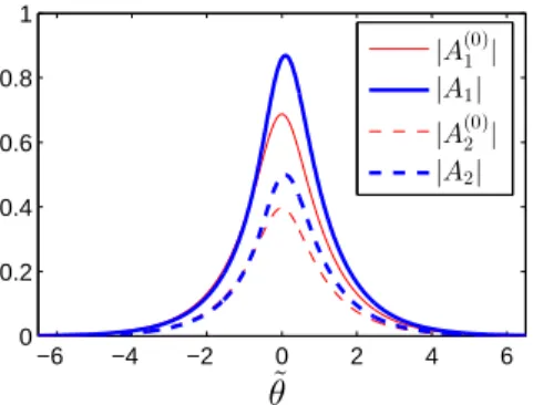
In Fig. 5.1 an example of a solution A1,2 of (4.3) is plotted together with the solution A⁽⁰⁾_1,2 in (5.1), from which the homotopy continuation was started. Note that while |A⁽⁰⁾_1,2| are even in ˜θ, the profiles |A1,2| are not symmetric. This lack of symmetry is caused by Im(β)6= 0 and Im(γ)6= 0. As easily checked, when Im(β) = 0 and Im(γ) = 0, then (4.3) has the symmetryA1,2(˜θ)→A1,2(−θ). While if Im(β)˜ 6= 0 or Im(γ)6= 0, this symmetry is lost.

−6 −4 −2 0 2 4 6

0 0.2 0.4 0.6 0.8 1

θ ˜

|A⁽⁰⁾₁ |

|A1|

|A⁽⁰⁾2 |

|A2|

Fig. 5.1.The solutions|A1,2|of (4.3)withcg= 1, κ= 0.5, κs= 0, α= 1, β= 0.3(1 + i) and γ = 0.2(1 + i), and the solutions |A⁽⁰⁾_1,2| in (5.1) with cg = 1, κ = 0.5, α = 1 and δ=π/2, v= 0.5, from whichA1,2 were computed by homotopy continuation.

6. Numerical Results on Moving Gap Solitons. We compare the asymp- totic approximation

√εu0(x, t) :=√ ε

2

X

j=1

Aj(εx, εt)φj(x)e^−iω0t

and a numerical approximation of (1.2) with the initial conditionu(x,0) =√εu0(x,0).

The integration of (1.2) is performed by the second order split step method (Strang splitting), where the PNLS (1.2) is split according to∂tu=Lu+N(u) withL= i∂_x² andN(u) =−iV(x)u−iσ|u|². The linear problem∂tu=Luis then solved in Fourier space via fft and the nonlinear problem∂tu=N(u) is solved exactly [19]. We use a large computational domain such that the solution tails at the boundary stay below 10⁻⁵ in (relative) amplitude. For the spatial discretization we usedx= 0.1 and for time steppingdt= 0.01.

In both examples below we study gap solitons in the gap bifurcating from the intersection of band functions ω±(k) at (k0, ω0) ≈ (0,3.428) for potentials V(x) = VFB(x; 1,1/2) +εW(x), see Fig. 2.2.

6.1. Odd PerturbationW(x). In this example we choose the odd perturbation W(x) = sin(4πx/d)

so thatκs= 0 in (4.3).

Numerically obtained values of the CME coefficients are cg≈3.3666546, κ≈0.4934402,

α≈0.1357055, β≈i 6.4865707∗10⁻⁷, γ ≈7.2199824∗10⁻⁶. (6.1) In Fig. 6.1the convergence of theL²-errorku(·, t)−√εu0(·, t)k^L2 at t=ε⁻¹ is shown. The four values of the velocity parameterv∈ {0,0.5,0.9,0.99}in the moving frame variable ˜θ are tested. In all cases the observed convergence rate is close toε¹ as predicted by the formal asymptotics (4.4). Note that the relative error is of the same asymptotic order as the absolute error due to the fact that the error consists of terms of the form√εf(εx)g(x) and becausek√εf(ε·)k^L2(R)=kfk^L2(R)for allε >0.

10⁻² 10⁻¹

10⁻²

ε v= 0 ku(·, ε⁻¹)−

√εu0(·, ε⁻¹)kL²

Cε^0.99

10⁻² 10⁻¹

10⁻²

ε v= 0.5 ku(·, ε⁻¹)−√εu0(·, ε⁻¹)kL²

Cε^0.97

10⁻² 10⁻¹

10⁻² 10⁻¹

ε v= 0.9 ku(·, ε⁻¹)−√εu0(·, ε⁻¹)kL²

Cε^0.99

10⁻² 10⁻¹

10⁻¹

ε v= 0.99

ku(·, ε⁻¹)−√εu0(·, ε⁻¹)kL²

Cε^0.96

Fig. 6.1.Convergence of theL²-error att=ε⁻¹, i.e. ofku(·, ε⁻¹)−√

εu0(·, ε⁻¹)kL², for the choice ofV_FB(x; 1,1/2) given in (2.6) andW(x) = sin ^4πx_d

,k0= 0, ω0 ≈3.428. Four velocity parameters inA1,2 are tested: v= 0,0.5,0.9,and0.99. The slopes of the full lines are obtained by interpolations of all the computed error values except for v = 0.99, where only the four smallest values are interpolated.

Although the values ofβ andγ in (6.1) are very small, a numerical test confirms that they are nonzero. Indeed, settingβ=γ= 0 in the computation of the envelopes A1,2 and studying once again ku(·, ε⁻¹)−√εu0(·, ε⁻¹)k^L2 with the new initial data u(x,0) =√εu0(x,0) produces a slower convergence rate, approximatelyε^0.69, see Fig.

6.2.

10⁻² 10⁻¹ 10⁻²

ε v= 0 ku(·, ε⁻¹)−

√εu0(·, ε⁻¹)kL²

Cε^0.69

Fig. 6.2. The error convergence as in Fig. 6.1 for the case v = 0 but ignoringβ and γ (setting β =γ = 0) in the gCMEs (4.3). Clearly, a slower convergence and larger error values are produced.

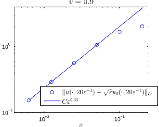
In order to test the behavior at very large times, the numerical error analysis has been performed for v = 0.9 also at t = 20ε⁻¹ with the resulting convergence rate O(ε^0.93), see Fig. 6.3.

10⁻² 10⁻¹

10⁻¹ 10⁰

ε v= 0.9

ku(·,20ε⁻¹)−

√εu0(·,20ε⁻¹)kL²

Cε^0.93

Fig. 6.3. The error convergence for the same setting as in Fig. 6.1 andv= 0.9at the large timet= 20ε⁻¹.

Fig. 6.4shows the modulus of the numerical solutionuas well as of the asymptotic approximation√ε|u0|att= 0 and a timet=O(ε⁻¹) for the four velocity parameters v from Fig6.1. For negative values ofv the modulus profiles are identical. Note that mainly for small values of v the large width of the pulses compared to the period of V makes it difficult to visually distinguish individual oscillations inuandu0.

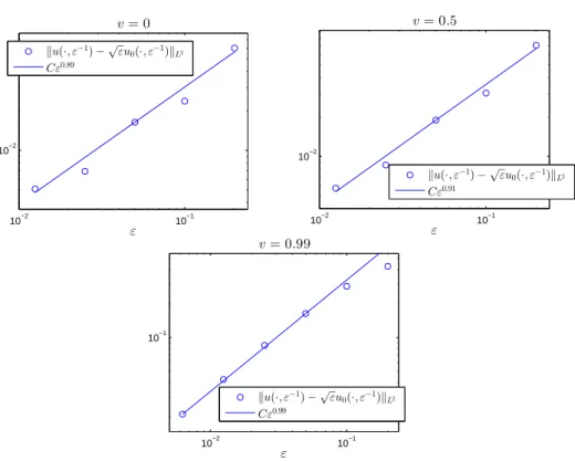
6.2. Even Perturbation W(x). As a second example we choose W(x) = cos(4πx/d)

and study, once again, gap solitons in the gap bifurcating from the intersection of band functions at (k0, ω0)≈(0,3.428). We obtain

cg≈3.3666546, κ≈0.4934402, κs≈0.0048743,

α≈0.1357055, β≈ −6.4865469∗10⁻⁴, γ≈ −7.2277824∗10⁻⁶.

−500 0 500 0

0.05 0.1 0.15 0.2 0.25 0.3 0.35

x (a)v= 0, ε= 0.05

t= 0, t=ε⁻¹

|u|

−3000 −2000 −1000 0 1000 2000

0 0.05 0.1 0.15 0.2

x (b)v= 0.5, ε= 0.025

t= 0 t= 40ε⁻¹

√ε|u0|

|u|

−20000 −1500 −1000 −500 0 500 0.02

0.04 0.06 0.08 0.1 0.12 0.14

x (c)v= 0.9, ε= 0.025

t= 0 t= 10ε⁻¹

√ε|u0|

|u|

−300 −200 −100 0 100 200 300 0

0.01 0.02 0.03 0.04 0.05 0.06 0.07

x

(d)v= 0.99, ε= 0.025

t= 0 t= 2ε⁻¹

√ε|u0|

|u|

Fig. 6.4.The numerical solution|u|and the asymptotic solution√

ε|u0|att= 0and at a timet=O(ε⁻¹) for the same setting as in Fig. 6.1. In (a) the approximation √ε|u0|at t= 0as well as att=ε⁻¹ are optically indistinguishable from|u(x, ε⁻¹)|.

An analogous convergence test to that in Sec. 6.1produces convergence rates between O(ε^0.9) andO(ε¹), see Fig. 6.5.

7. Conclusions. Using a formal asymptotic analysis and numerical tests of con- vergence of the approximation error with respect to the asymptotic parameter, it is shown that periodically perturbed finite band potentials of finite contrast in one di- mension support a family of approximate moving gap solitons. The frequency param- eter of the gap solitons lies in a narrow gap generated by the periodic perturbation (of amplitude 0< ε ≪1). The gaps open from transversal crossings of band func- tions and the Bloch waves at a bifurcation point thus carry a nonzero group velocity.

The problem of selection of the Bloch waves out of the two dimensional eigenspace is solved by an optimization algorithm.

While existing results on gap solitons in finite contrast structures produce only gap solitons with infinitesimal velocity, the new gap solitons propagate at anO(1) velocity across the periodic structure. The convergence tests confirm theε¹-convergence rate of the L²-error on time scales of O(ε⁻¹) as expected from the formal asymptotics.

Rigorous estimates of the approximation error will be the subject of a future paper.

REFERENCES

[1] M. J. Ablowitz and Z. H. Musslimani. Spectral renormalization method for computing self- localized solutions to nonlinear systems.Opt. Lett., 30(16):2140–2142, 2005.

[2] M. Abramowitz and I. Stegun.Handbook of Mathematical Functions: With Formulas, Graphs, and Mathematical Tables. Applied mathematics series. Dover, 1964.

10⁻² 10⁻¹ 10⁻²

ε v= 0 ku(·, ε⁻¹)−√

εu0(·, ε⁻¹)kL²

Cε^0.89

10⁻² 10⁻¹

10⁻²

ε v= 0.5

ku(·, ε⁻¹)−√

εu0(·, ε⁻¹)kL²

Cε^0.91

10⁻² 10⁻¹

10⁻¹

ε v= 0.99

ku(·, ε⁻¹)−

√εu0(·, ε⁻¹)kL²

Cε^0.99

Fig. 6.5. Convergence of the L²-error at t=ε⁻¹, i.e. ofku(·, ε⁻¹)−√εu0(·, ε⁻¹)kL², for the choice of VFB(x; 1,1/2) given in (2.6) and W(x) = cos ^4πx_d

, k0 = 0, ω0 ≈3.428.

Three gap soliton velocities are tested: v= 0,0.5, and0.99. The slopes of the full lines are obtained by interpolations of all the computed error values except forv= 0.99, where only the four smallest values are interpolated.

[3] A. B. Aceves and S. Wabnitz. Self induced transparency solitons in nonlinear refractive media.

Phys. Lett. A, 141:37–42, 1989.

[4] K. Busch, G. Schneider, L. Tkeshelashvili, and H. Uecker. Justification of the nonlinear Schr¨odinger equation in spatially periodic media. Z. Angew. Math. Phys., 57:905–939, 2006.

[5] C. M. de Sterke, D. G. Salinas, and J. E. Sipe. Coupled-mode theory for light propagation through deep nonlinear gratings. Phys. Rev. E, 54:1969–1989, 1996.

[6] T. Dohnal and T. Hagstrom. Perfectly matched layers in photonics computations: 1d and 2d nonlinear coupled mode equations.J. Comput. Phys., 223(2):690–710, 2007.

[7] T. Dohnal, D. E. Pelinovsky, and G. Schneider. Coupled-mode equations and gap solitons in a two-dimensional nonlinear elliptic problem with a separable periodic potential.J. Nonlin.

Sci., 19:95–131, 2009.

[8] T. Dohnal and H. Uecker. Coupled mode equations and gap solitons for the 2d Gross-Pitaevskii equation with a non-separable periodic potential.Physica D, 238(9-10):860–879, 2009.

[9] M. Eastham. Spectral Theory of Periodic Differential Equations. Scottish Academic Press, Edinburgh London, 1973.

[10] R. H. Goodman, M. I. Weinstein, and P. J. Holmes. Nonlinear propagation of light in one- dimensional periodic structures. J. Nonlin. Sci., 11(2):123–168, 2001.

[11] T. Kat¯o. Perturbation theory for linear operators. Grundlehren der mathematischen Wis- senschaften. Springer, Berlin, 1995.

[12] W. Magnus and S. Winkler. Hill’s Equation. Interscience, New York, 1966.

[13] R. S. Maier. Lam´e polynomials, hyperelliptic reductions and Lam´e band structure.Phil. Trans.

R. Soc. A, 366:1115–1153, 2008.

[14] D. Pelinovsky. Localization in Periodic Potentials: From Schr¨odinger Operators to the Gross- Pitaevskii Equation. London Mathematical Society Lecture Note Series. Cambridge Uni-

versity Press, 2011.

[15] D. E. Pelinovsky and G. Schneider. Justification of the coupled-mode approximation for a nonlinear elliptic problem with a periodic potential.Appl. Anal., 86:1017–1036, 2007.

[16] D. E. Pelinovsky and G. Schneider. Moving gap solitons in periodic potentials. Math. Meth.

Appl. Sci., 31:1099–1476, 2008.

[17] M. Reed and B. Simon. Methods of Modern Mathematical Physics. IV. Analysis of Operators.

Academic Press, New York, 1978.

[18] G. Schneider and H. Uecker. Nonlinear coupled mode dynamics in hyperbolic and parabolic periodically structured spatially extended systems.Asymptot. Anal., 28(2):163–180, 2001.

[19] J. A. C. Weideman and B. M. Herbst. Split-step methods for the solution of the nonlinear Schr¨odinger equation. SIAM J. Num. Anal., 23(3):485–507, 1986.

2013-05 Tom´ aˇ s Dohnal

Traveling Solitary Waves in the Periodic Nonlinear Schr¨ odinger Equation with Finite Band Potentials

2013-04 Karl Friedrich Siburg, Pavel Stoimenov, and Gregor N.F. Weiß

Forecasting Portfolio-Value-at-Risk with Nonparametric Lower Tail Dependence Estimates 2013-03 Martin Heida

ON THERMODYNAMICS OF FLUID INTERFACES 2013-02 Martin Heida

EXISTENCE OF SOLUTIONS FOR TWO TYPES OF GENERALIZED VERSIONS OF THE CAHN-HILLIARD EQUATION

2013-01 T. Dohnal, A. Lamacz, B. Schweizer

Dispersive effective equations for waves in heterogeneous media on large time scales 2012-19 Martin Heida

On gradient flows of nonconvex functionals in Hilbert spaces with Riemannian metric and application to Cahn-Hilliard equations 2012-18 R.V. Kohn, J. Lu, B. Schweizer, and M.I. Weinstein

A variational perspective on cloaking by anomalous localized resonance 2012-17 Margit R¨ osler and Michael Voit

Olshanski spherical functions for infinite dimensional motion groups of fixed rank 2012-16 Selim Esedo¯ glu, Andreas R¨ atz, Matthias R¨ oger

Colliding Interfaces in Old and New Diffuse-interface Approximations of Willmore-flow 2012-15 Patrick Henning, Mario Ohlberger and Ben Schweizer

An adaptive multiscale finite element method

2012-14 Andreas Knauf, Frank Schulz, Karl Friedrich Siburg Positive topological entropy for multi-bump magnetic fields 2012-13 Margit R¨ osler, Tom Koornwinder, and Michael Voit

Limit transition between hypergeometric functions of type BC and Type A 2012-12 Alexander Schnurr

Generalization of the Blumenthal-Getoor Index to the Class of Homogeneous Diffusions with Jumps and some Applications

2012-11 Wilfried Hazod

Remarks on pseudo stable laws on contractible groups 2012-10 Waldemar Grundmann

Limit theorems for radial random walks on Euclidean spaces of high dimensions 2012-09 Martin Heida

A two-scale model of two-phase flow in porous media ranging from porespace to the macro scale

2012-08 Martin Heida

On the derivation of thermodynamically consistent boundary

conditions for the Cahn-Hilliard-Navier-Stokes system

Uniform oscillatory behavior of spherical functions of GL

/U

at the identity and a central limit theorem

2012-06 Agnes Lamacz and Ben Schweizer

Effective Maxwell equations in a geometry with flat rings of arbitrary shape 2012-05 Frank Klinker and G¨ unter Skoruppa

Ein optimiertes Gl¨ attungsverfahren motiviert durch eine technische Fragestellung 2012-04 Patrick Henning, Mario Ohlberger, and Ben Schweizer

Homogenization of the degenerate two-phase flow equations 2012-03 Andreas R¨ atz

A new diffuse-interface model for step flow in epitaxial growth 2012-02 Andreas R¨ atz and Ben Schweizer

Hysteresis models and gravity fingering in porous media 2012-01 Wilfried Hazod

Intrinsic topologies on H-contraction groups with applications to semistability 2011-14 Guy Bouchitt´ e and Ben Schweizer

Plasmonic waves allow perfect transmission through sub-wavelength metallic gratings 2011-13 Waldemar Grundmann

Moment functions and Central Limit Theorem for Jacobi hypergroups on [0, ∞[

2011-12 J. Koch, A. R¨ atz, and B. Schweizer

Two-phase flow equations with a dynamic capillary pressure 2011-11 Michael Voit

Central limit theorems for hyperbolic spaces and Jacobi processes on [0, ∞[

2011-10 Ben Schweizer

The Richards equation with hysteresis and degenerate capillary pressure 2011-09 Andreas R¨ atz and Matthias R¨ oger

Turing instabilities in a mathematical model for signaling networks 2011-08 Matthias R¨ oger and Reiner Sch¨ atzle

Control of the isoperimetric deficit by the Willmore deficit 2011-07 Frank Klinker

Generalized duality for k-forms

2011-06 Sebastian Aland, Andreas R¨ atz, Matthias R¨ oger, and Axel Voigt Buckling instability of viral capsides - a continuum approach

2011-05 Wilfried Hazod

The concentration function problem for locally compact groups revisited: Non-dissipating space-time random walks, τ-decomposable laws and their continuous time analogues 2011-04 Wilfried Hazod, Katrin Kosfeld

Multiple decomposability of probabilities on contractible locally compact groups 2011-03 Alexandra Monzner* and Frol Zapolsky†

A comparison of symplectic homogenization and Calabi quasi-states