Threshold Resummation Studies for Polarized and Unpolarized High-pT

Polarized and Unpolarized High-

Hadron Production at COMPASS

Dissertation

zur Erlangung des

Doktorgrades der Naturwissenschaften (Dr. rer. nat)

der Fakult¨at f¨ur Physik der

Universit¨at Regensburg

vorgelegt von

Claudia Uebler

aus Vilshofen

im Jahr 2019

Das Promotionsgesuch wurde am 22. Januar 2019 eingereicht.

Pr¨ufungsausschuss:

Vorsitzender: Prof. Dr. C. Sch¨uller 1. Gutachter: Prof. Dr. A. Sch¨afer 2. Gutachter: Prof. Dr. W. Vogelsang Weiterer Pr¨ufer: Prof. Dr. K. Richter

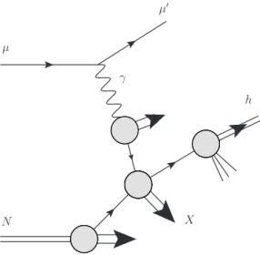
duction in longitudinally polarized lepton-nucleon scattering µN →µ⁰hX at COMPASS.

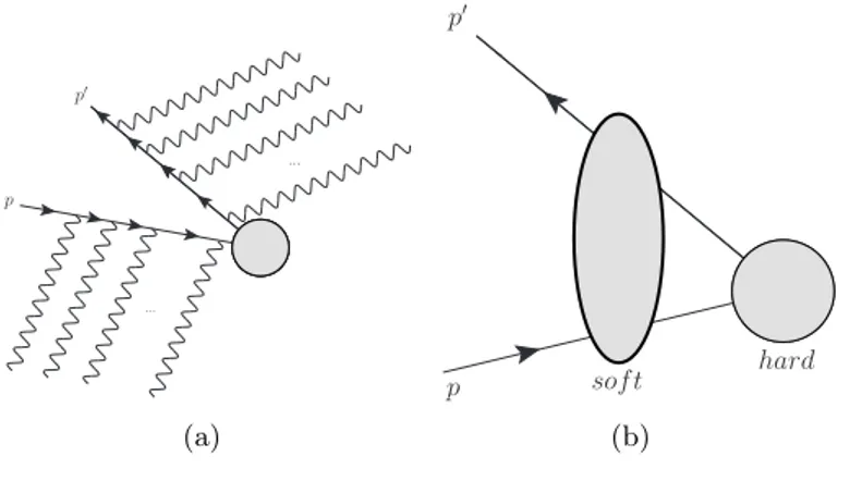
The goal is to address threshold resummation effects to double-longitudinal spin asymme- tries at COMPASS kinematics. At these kinematics, nearly all available energy is used for the production of the high-p_T parton and its recoiling counterpart. In that case, the phase space for additional radiation of partons becomes small, resulting in large logarithmic QCD corrections at every order in perturbation theory. These logarithmic contributions spoil the perturbative expansion, and thus have to be resummed. Using threshold resumma- tion techniques in Mellin momentum N space, we are able to deal with those logarithmic corrections up to all perturbative orders inα_s at a certain logarithmic level. In our calcu- lations we choose next-to-leading logarithmic accuracy. Further, we develop a framework to include subleading 1/N-suppressed logarithms into future calculations.

In our phenomenological results for COMPASS we present a detailed study of the im- pact of next-to-leading logarithmic threshold resummation on the spin-dependent cross section and on the corresponding double-longitudinal spin asymmetryA_LLfor the high-p_T photoproduction process µN → µ⁰hX. We include resummation for the direct, as well as for the resolved-photon contribution. In a comparison of the spin-averaged with the spin-dependent cross sections we find out that the latter receives smaller corrections from resummation than the spin-averaged one, indicating that threshold corrections do not can- cel in the double-spin asymmetry and rather tend to decrease it, yielding an overall better agreement between experiment and theory.

Finally, we reveal that the parton-to-hadron fragmentation functions have a strong impact on the size and shape of the predicted spin asymmetries.

1. Introduction 1 2. Foundations of Perturbative Quantum Chromodynamics 7

2.1. Lagrangian of Quantum Chromodynamics . . . 7

2.2. The Group SU(3) . . . 9

2.3. Asymptotic Freedom and the Running Coupling . . . 9

2.4. Regularization and Renormalization . . . 12

3. Parton Distribution and Fragmentation Functions 15 3.1. Factorization Theorem . . . 15

3.2. Parton Distribution and Fragmentation Functions . . . 17

3.3. Parton Structure of the Photon . . . 21

4. Foundations of Threshold Resummation 25 4.1. Exponentiation for (Non-)Abelian Gauge Theories . . . 26

4.1.1. Exponentiation of Soft Photons . . . 26

4.1.2. Exponentiation of Soft Gluons . . . 28

4.2. Phase Space Factorization in Mellin Moment Space . . . 33

4.3. Threshold Resummation in Mellin Space . . . 34

4.4. Threshold Corrections for Single-Particle Inclusive Cross Section . . . 36

4.4.1. Refactorization . . . 37

4.4.2. Radiative Factors . . . 40

5. Threshold Resummation for Single-Inclusive Hadron Production 45 5.1. Theoretical Framework . . . 46

5.2. Transformation to Mellin Moment Space . . . 51

5.3. NLL-Resummed Hard-Scattering Function . . . 52

5.3.1. Exponents at NLL . . . 55

5.3.2. Hard- and Soft-Matrices . . . 57

5.4. NLO Calculation . . . 60

5.5. Extraction of the Coefficients . . . 63

5.6. Inverse Mellin Transform and Matching Procedure . . . 63

5.7. Double-Spin Asymmetry . . . 64

6. Subleading Contributions 67 6.1. Formalism to Calculate Subleading Mellin-Contributions . . . 67

6.2. Subleading Logarithms for NLO Cross Sections . . . 71

6.3. Subleading Logarithms for Threshold Resummation . . . 80

i

7. Phenomenological Results for COMPASS 85

7.1. Polarized and Unpolarized Resummed Cross Sections . . . 87

7.1.1. Polarized Unidentified Hadron Production from a Deuteron . . . 87

7.1.2. Pion and Kaon Production . . . 94

7.2. Double-Spin Asymmetry . . . 96

8. Conclusion and Outlook 103 A. Feynman Rules 107 B. Hard, Soft and Γ-Matrices 111 B.1. Soft Matrices . . . 111

B.2. Anomalous Dimension Matrices . . . 112

B.3. Hard Matrices . . . 113

C. Coefficients 117

Bibliography 119

Introduction 1

In the last 100 years knowledge of the proton structure has grown a lot. The story of the proton and with that its discovery starts with Rutherford’s proof that the hydrogen nucleus is present in other nuclei [1]. Then, 1922 the idea ofspin was introduced through the Stern-Gerlach experiment [2, 3] to construe the observations. That the proton is a spin-1/2 fermion was concluded five years later [4]. A series of experiments started to deepen the knowledge of the proton structure, and with that Hofstadter and McAllister made first measurements of the RMS radius for the charge and magnetic moment of pro- tons in 1955 [5]. Then, in the 1960s, Ne’eman [6] and Gell-Mann [7] classified hadrons through the Eightfold Way, a SU(3) flavor symmetry. A quark model was introduced by Gell-Mann and Zweig [8] stating that hadrons were consisting of three quark types, named up, down and strange quarks, to which one referred properties as spin and electric charge. The experimental breakthrough followed in 1968, when a deep inelastic scatter- ing (DIS) experiment at the Stanford Linear Accelerator Center (SLAC) discovered that protons and neutrons are indeed built up by smaller constituents called partons. All the developments of experimental and theoretical work in the 1960’s and 1970’s led finally to the theory of Quantum Chromodynamics (QCD) as we know it today. With that, one is able to describe the dynamics of quark and gluon constituents in the hadrons. QCD, as a non-abelian quantum field theory, describes the strong interaction using the concept of color charged quarks and gluons. It is part of the standard model and exhibits the crucial properties of asymptotic freedom and confinement, whereby quarks are bound strongly in the hadrons at larger distances and behave asymptotically free at short distances. How- ever, there are still open questions left.

A lot of effort has been applied to find answers to the question of how the gluon and quark spins and orbital angular momenta combine to generate the nucleon spin of 1/2. The familiar assumption that protons are made up of twouand onedquark constituents gen-

1

erate a naively expectation that the quarks carry about a third of the proton momentum.

However, the proton structure and momentum distribution is another one, as protons con- tain additional gluons and low-momenta quarks and antiquarks called sea quarks. Lattice QCD even states that the proton mass is largely determined by the binding energy of the gluons. How the total proton spin is distributed among its quark, antiquark and gluon constituents, among the polarizations and angular momenta, is still an outstanding ques- tion. Measurements from the EMC experiment [9] in the 1980s mark the starting point of the so-called “proton spin crisis”, where a series of experiments provided increasingly precise results, revealing the surprising discovery that only about 30% of the nucleon spin is built up from the polarization of quarks and anti-quarks combined. While lattice cal- culations [10] give rise to the assumption that the missing 70% is not provided by the quark orbital angular momentum alone, RHIC [11, 12], a polarized proton-proton collider, even indicates that the gluon polarization contributes significantly to the total spin. The proton helicity sum rule [13–15] reads

1 2 = 1

2∆Σ + ∆G+L^q_z+L^g_z, (1.1)

where 1/2∆Σ = 1/2R1 0 dx

∆u+ ∆¯u+ ∆d+ ∆ ¯d+ ∆s+ ∆¯s

(x) denotes the quark spin contribution andL^qz+L^gz labels the total orbital angular momenta of quarks and gluons.

Further, integrating the gluon distribution ∆g(x) over all momentum fractions x (and summing over flavors), we obtain the gluon spin contribution ∆G = R1

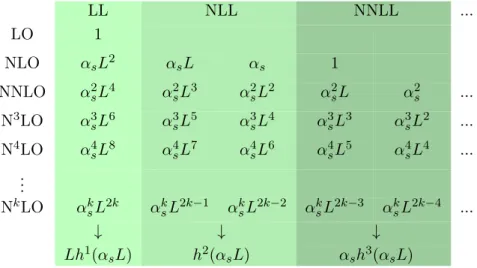
0 dx∆g(x). This highlights that ∆g is a key ingredient for solving the proton spin puzzle. One of the main tools to gain information about the gluon distribution are thespin asymmetries, which are directly sensitive to ∆g. The COMPASS experiment [16, 17], short for Common Muon and Proton Apparatus for Structure and Spectroscopy, at the Super Proton Synchrotron SPS, considers semi-inclusive hadron production of the type

µN →µ⁰hX . (1.2)

COMPASS has already presented results for the spin-averaged cross section a while ago [18]

and more recently also data for the corresponding double-longitudinal spin asymmetry ALL [19, 20]. In these reactions the hard scale is set by the transverse momentum of the produced hadron which is for COMPASS kinematics much smaller than for ∆g(x, Q²) determinations by, e.g. inclusive jet and di-jet production at RHIC, see [12]. Both sets of experiments are complementary as one needs a large kinematic reach to analyze the evolution of polarized parton distributions. High precision is needed, as the systematic theoretical uncertainties of the analyses has to be much smaller than the experimental uncertainties. If the theoretical framework is adequate for describing the photoproduc- tion γN → hX in the kinematic regime relevant at COMPASS, analyzing the data may give reliable information on ∆g. Hard photoproduction processes are well understood,

in particular the connection between direct and resolved photon contributions [21]. The quasi-real photon can interact on the one hand as pointlike particle couplingdirectly with a parton from the nucleon, on the other hand it can beresolved into its partonic content and it can couple through quantum fluctuations containing quarks, antiquarks and gluons.

However, threshold resummation, which is required at COMPASS kinematics [22], is an additional feature which is less standard. For large enough transverse momentum of the observed hadron, perturbative methods and in particular threshold resummation tech- niques can be applied. The theoretical calculations start at orderO(ααs), which is thus what we mean with Leading Order (LO), with the electromagnetic and strong coupling constantsα andα_s, while next-to-leading order (NLO) meansO(αα²_s). NLO QCD correc- tions without resummation are presented for the double-spin asymmetry in Refs. [23–25].

However, for COMPASS kinematics whereat one is close to kinematic threshold, large QCD corrections appear. The reason is that nearly all available energy is used for the production of the high-pT parton and its recoiling counterpart. Then, the phase space for additional radiation of partons becomes small, and after the incomplete cancelation of infrared divergences between real and virtual diagrams large logarithmic corrections can be observed at every order in perturbation theory [26, 27], starting at NLO. Atn-th order logarithmic corrections up to

αⁿ_s

ln²ⁿ⁻¹(1−z) 1−z

+

, (1.3)

appear and are accompanied by lower, subleading powers of logarithms. Here,zlabels the threshold region, hence when z→1 no further energy is left for additional radiation.

In every higher order of perturbation theory two additional powers of these logarithms emerge and spoil the perturbative expansion [28]. Thus, these threshold logarithms can- not be neglected and require to be resummed to all orders of perturbation theory [29–36].

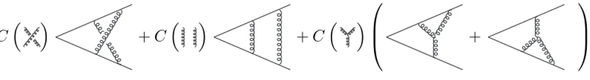
Using the techniques of threshold resummation we include logarithms in our following calculations up to next-to-leading logarithmic (NLL) accuracy, containing the three lead- ing “towers”αⁿ_s

ln²ⁿ⁻¹(1−z)/(1−z)

+ at leading-logarithmic (LL) accuracy, as well as α^k_s

ln²ⁿ⁻²(1−z)/(1−z)

+, and further αⁿ_s

ln²ⁿ⁻³(1−z)/(1−z)

+ at NLL.

With this technique at hand we want to study the semi-inclusive photoproduction process µN →µ⁰hX with hadron production at high transverse momentum p_T for both cases, di- rect and resolved photons, calculating spin-dependent threshold resummed cross sections involving longitudinally polarized nucleons and photons. This denotes an extension to the calculations of Ref. [22], where the unpolarized cross sections have been calculated using threshold resummation methods. There, one could find that the resummed cross section shows a markedly better agreement with the experimental results than the next-to-leading order one.

Although resolved subprocesses show an equivalent structure to hadronic scatteringpp→ hX which has been already investigated even for the spin-dependent case, see Ref. [27],

we will use a different framework. Ref. [27] integrates over all rapidities of the produced hadron, and therefore the cross section takes, after a transformation into Mellin moment space, the form of a complete convolution with parton distribution functions. Contrary to that we will perform in the following threshold resummation at arbitrary fixed rapid- ity, using techniques developed in [22, 37]. This implies that only the resummed cross section convoluted with the fragmentation function is transformed into Mellin-N space, however, the parton distribution functions stay in physical space. Our main goal is then the study of the double-longitudinal spin asymmetry ALL at COMPASS kinematics, and in this instance the investigation of the relevance of higher-order QCD threshold correc- tions. For that we compare our theoretical calculations with the experimental results of COMPASS [19, 20]. Note that there have been assumptions that higher-order perturba- tive corrections cancel in the ratios of spin-dependent and spin-averaged cross sections, i.e. for spin asymmetries,

A_LL = d∆σ

dσ . (1.4)

However, as we will see, this assumption is incorrect and higher-order threshold correc- tions cannot be neglected for the calculation ofALL.

The thesis is organized as follows. In Chap. 2 we give a short overview of the principles of perturbative Quantum Chromodynamics. However, we refer to some standard textbooks or reviews for more details. Then, as factorization is a main ingredient for our following calculation, we will investigate in Chap. 3 the underlying ideas and illuminate further parton distribution and fragmentation functions. With that we will also shed light on the parton structure of the photon which will be needed for the resolved photon contri- butions. After this we are ready to review the foundations of threshold resummation in Chap. 4. We will start with an exponentiation formula for (non-)abelian gauge theories, focusing first on photons and then on gluons. This is followed by an introduction into the Mellin moment space, which is necessary for threshold resummation. We want then proceed with an explicit derivation of the radiative resummation exponents. For that, refactorization will be the underlying technique. These exponents will be needed in Chap.

5, when we arrive at the threshold resummation for single-inclusive hadron production at COMPASS. In this chapter, the theoretical framework is given, and besides the formula of the resummed hard-scattering function at next-to-leading logarithmic order, we will also consider the fixed-order case. With the help of a matching procedure we will then include full NLO results in our theoretical results, to provide highest available precision. While we are restricting ourselves for our phenomenological studies at next-to-leading logarithmic level neglecting 1/N-suppressed logarithms, we investigate in Chap. 6 a framework, how to compute those subleading contributions and provide them explicitly for the fixed-order calculation. Further we show which terms in the threshold resummed calculation could generate lnN/N terms. Our phenomenological results for COMPASS will then be shown

in Chap. 7 and our double-longitudinal spin asymmetries will be compared with the ex- perimental data. We will compare our results for different fragmentation function sets and consider protons and deuterons as targets. Studying the role of higher-order QCD corrections at kinematic threshold and comparing the unpolarized with the polarized cal- culated cross sections, we find important conclusions concerning the double-longitudinal spin asymmetry. Finally, in Chap. 8 we finish the thesis with a conclusion and an outlook.

In addition to that, an appendix is available with further details.

Note that parts of our studies are already published and can be found in our papers [38]

and [39], however, the detailed calculations and many details are provided in the following.

Emilie du Chˆ´ atelet

Foundations of Perturbative Quantum 2

Chromodynamics

In this chapter we want to introduce the main basics of perturbative Quantum Chromo- dynamics (QCD), serving as a starting point for the calculations in the following chapters.

As this overview will be rather short, we point to some standard text books [40–43] or to Ref. [44] for further details. In the following we want to give a brief review of the Lagrangian of QCD, which is essential to derive the Feynman rules given in the Appendix A.

2.1. Lagrangian of Quantum Chromodynamics

Quantum Chromodynamics (QCD) is a non-abelian gauge theory describing the strong force which is one of the four fundamental forces. It is part of the Standard Model and describes the interaction between quarks and gluons, which carry color. The gauge invariant Lagrangian,

L=

Nf

X

f

Ψ¯_f,a iγ^µ∂µδ_ab−gγ^µt^C_abA^C_µ −m_fδ_ab

Ψ_f,b−1

4F_µν^AF^Aµν+Lgf+LF P (2.1)

=

Nf

X

f

Ψ¯_f i /D−m_f

Ψ_f −1

4F_µν^AF^Aµν

| {z }

Lcl

+Lgf+LF P,

is invariant under Lorentz transformations and describes how quarks interact with each other by exchanging gluons, the latter of which are massless gauge bosons building up an octet in the adjoint representation of SU(3). It consists of the classical Lagrangian Lcl, a

7

gauge-fixing partLgf and aFaddeev-Popov ghost part L^{F P}. InLcl, Ψ_f,a denotes the field spinors for quarks with flavor f, mass m_f and colora, with arunning from 1 toN_c= 3.

Further the covariant derivative is

Dµ=∂µ−igt^CA^C_µ. (2.2)

Repeated indices are understood to be summed over and the Dirac matricesγµ satisfy the Dirac algebra, an anti-commutation relation reading

{γ^µ, γ^ν}= 2g^µν. (2.3)

The field strength tensor,

F_µν^A =∂µA^A_ν −∂νA^A_µ −gfABCA^B_µA^C_ν, (2.4) is constructed from the gluon fields A^A_µ, where A runs from 1 to N_c²−1 = 8. The term

−¹₄F_µν^AF^Aµν describes their self-interaction as gluons carry color themselves, and differs from the field strength tensor of QED by the last term gf_ABCA^B_µA^C_ν, which gives rise to the three- and four-gluon interaction. The fABC are the structure constants of the SU(3) group andgis the strong coupling constant. Withf_ABC and the eight independent generators t^A of the SU(3) group, which correspond to 3×3 hermitian matrices, the Lie algebra is defined through the commutation relation

t^A, t^B

=if_ABCt^C. (2.5)

Gluon emission from a quark can be identified with the color factorC_F ≡(N_c²−1)/(2N_c) = 4/3, which is given by the relationt^A_abt^A_bc=CFδac. Further, gluon emission from a gluon is associated with the color factorC_A=N_c= 3, which can be found inf^ABCf^BCD =C_Aδ_AD, and finally we have the color factorT_R= 1/2 when a gluon splits into a quark-antiquark pair given int^A_abt^B_ab=TRδAB. What is still missing is on the one side the gauge-fixing term Lgf, and on the other side the ghost-field term LF P. The necessity for Faddeev–Popov ghosts follows from the quantization of the classical Lagrangian. For the specific gauge

∂µA^Aµ = 0, the gauge fixing term is given by Lgf =−1

2ξ(∂µA^Aµ)(∂νA^Aν). (2.6) Here, the parameter ξ can be chosen freely without changing the physical results, which are independent of the gauge used in a calculation. A common choice is the Feynman (or Feynman-t’Hooft) gauge, where the gauge parameter isξ= 1. These additional ghost fields χ^A have to be introduced to solve an overcounting issue in the quantization of the

theory. Their Lagrangian reads for the gauge∂µA^Aµ = 0:

LF P =gf_ABCχ¯^A∂^µ(A^C_µχ^B)−χ¯^A∂^µ∂µχ^A. (2.7) Note that Faddeev-Popov ghost fields do not describe physical particles and have their own Feynman rules.

2.2. The Group SU(3)

Let us now go on to classify Quantum Chromodynamics in a bit more mathematical way.

It is a SU(3) gauge theory and part of the SU(3)×SU(2)×U(1) Standard Model, where SU(2)×U(1) represents the unification of the weak interaction and the electromagnetic interaction. In the former leptons interact via three massive gauge bosons (W^± and Z⁰) whereas the electromagnetic force is mediated by massless photons. In the case of the group SU(3) = SU(3)_color of QCD, one findsN_c²−1 = 8 massless gauge bosons, the gluons which appear in different so called colors. In contrast to the photon in QED which is a neutral spin-1 particle carrying no electrical charge, the gluons themselves carry color charge and can thus interact with each other. The gluons are described by eight vectorsA^A_µ in the adjoint representation of SU(3) and are therefore said to make up an octet. Quarks are described through spinors in the fundamental representation and build up a triplet.

The independent color states of the gluons are superpositions of different color-anticolor states and read:

(r¯b+b¯r)/√

2, −i(r¯b−b¯r)/√

2, (r¯g+g¯r)/√

2, −i(r¯g−g¯r)/√

2, (b¯g+g¯b)/√

2, −i(b¯g−g¯g)/√

2, (r¯r+b¯b)/√

2, (rr¯+b¯b−2g¯g)/√

6. (2.8)

The eight generators of SU(3) are related to the Gell-Mann matrices, a set of hermitian, traceless matrices collected in [43]:

t^A= λ^A

2 . (2.9)

The consequences of the gluon self-interaction will be discussed in the next section.

2.3. Asymptotic Freedom and the Running Coupling

Free partons that means quarks and gluons, have never been observed experimentally.

Unlike in QED where the elementary particles described by the Lagrangian can be observed directly, quarks and gluons are always bound in color singlet states referred to as hadrons.

QCD α

(M

) = 0.1181 ± 0.0011

pp –> jets

e.w. precision fits (N³LO)

0.1 0.2 0.3

α

(Q

)

1 10 100

Q [GeV]

Heavy Quarkonia (NLO)

e⁺e^– jets & shapes (res. NNLO)

DIS jets ^(NLO)

April 2016

τ decays (N³LO)

1000

(NLO

pp –> tt(NNLO)

(–) )

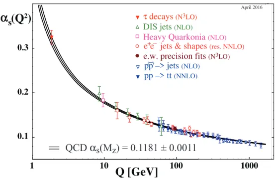
Fig. 2.1.: The coupling constantαs(Q) at an energy scaleQfrom different measurements. The used perturbative order is declared in the brackets, with NLO standing for next-to-leading order, and res. NNLO standing for next-to NLO matched with resummed next-to-leading logarithms. The figure is taken from Ref. [44].

In the following this feature will be discussed a bit more detailed following Refs. [44–46].

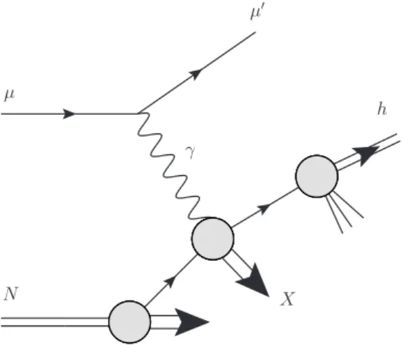
The self-interaction of gluons yields a gluon vacuum polarization, resulting inasymptotic freedom. This means that partons, which areconfined inside the “colorless” hadron, are treated to be asymptotically free in the asymptotic limit, so that perturbative methods are applicable. There, the coupling constantgorαs= _4π^g2, as one of the most fundamental parameters of this theory, decreases as the distance between two fields decreases, or in other words, decreases with increasing momentum transfer, see Fig. (2.1), taken from Ref. [44]. More precisely, the coupling constant can be written as a running coupling in terms of theβ-function, satisfying the renormalization group equation (RGE):

µr

dαs(µr)

dµ_r =β(αs(µr)) =− b0α²_s+b1α³_s+b2α⁴_s+...

, (2.10)

with the first three coefficients of theβ-function collected in [45], b0 = 11CA

12π −N_fT_R

3π = 33−2N_f 12π , b₁ = 1

24π² 17C_A² −10T_RC_AN_f −6T_RC_FN_f

= 153−19N_f 24π² , b₂ = 77139−15099N_f + 325N_f²

3456π³ . (2.11)

While the coefficientsb₀ andb₁ are independent of the renormalization scheme, all higher- order terms have a scheme-dependence. We adopt the MS scheme, where terms containing γE and ln(4π) are subtracted, which appear together with the (1/)-poles in dimensional regularization [40]. Note that the negative sign in theβ-function in Eq. (2.10) reflects the origin for asymptotic freedom: in hard processes, where the momentum transfer is large, the strong coupling becomes weak. This remains true as long asN_f <17, whenb₀changes its sign. Having a prediction forα_s(µ_r) at a given scale µ_r, one is able to determine the value of αs(µ) at any other scale. The behaviour described by Eq. (2.10) is an essential feature of the theory which makes it possible to use perturbation theory for the calculation of high energetic QCD processes. The main idea behind this is an expansion of physical observables in terms of the strong coupling which becomes small at high energies such that higher order terms can be neglected. Solving the differential equation in (2.10) exactly and analytically can only be done by neglecting all terms in theβ-function except b0 and b₁. This yields:

α_s(µ²) = 1

b₀ln(µ²/Λ_QCD). (2.12)

Here, ΛQCD is an integration constant which can be thought of as marking the transition between perturbative and non-perturbative scales. In particular at µ= Λ_QCD Eq. (2.12) diverges, marking the breakdown of perturbation theory. Approximate analytical solutions can be found even at 5-loop order, including b₅. A 3-loop solution, truncating all terms higher thanb₃ is reviewed in [44],

α_s' 1 b₀L

1−b₁

b²₀ lnL

L +b²₁(ln²L−lnL−1) +b₀b₂ b⁴₀L²

−b³₁ ln³L− ⁵₂ln²L−2 lnL+¹₂

+ 3b0b1b2lnL− ¹₂b²₀b3

b⁶₀L³

! +O

1 L⁵

, (2.13) with L ≡ ln(µ²/Λ_QCD). Then, we can also express the coupling at a given scale k² in

µ ν k+q

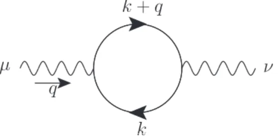
k q

Fig. 2.2.: Virtual electron-positron pair production from the vacuum polarization of a photon.

terms of the coupling at scaleµ², reading at first loop order:

αs(k²) = αs(µ²) 1 +b0αs(µ²) ln

k² µ²



1−b1

b₀

αs(µ²) 1 +b0αs(µ²) ln

k² µ²

ln

1 +b0αs(µ²) ln k²

µ²



. (2.14)

2.4. Regularization and Renormalization

In the next section we want to introduce theoretical methods for higher-order calcula- tions, in which unphysical divergent expressions appear. We distinguish between so called infrared divergences (IR) appearing in the low-momentum range, whenk→0, andultravi- olet divergences in the high-momentum region, when k→ ∞. Further, there are collinear singularities generated by collinear emissions. At this point we will briefly discuss how these divergent contributions can be handled consistently and refer to Refs. [40–43, 47] for more details.

Once an emitted parton has momentumk→0, infrared or soft singularities appear. Those divergences cancel when all contributions or diagrams of a given process or observable are summed up, in particular they cancel against bremsstrahlung diagrams where additional final photons or gluons with soft momentum are emitted. As soft radiation cannot be observed, the cross section for soft emissions is typically added to the one without soft radiation such that these soft singularities cancel, resulting in a divergence free, infrared safe, cross section.

Collinear singularities arising from the collinear emission of partons off initial or final-state partons are factorized into the bare parton distribution or fragmentation functions. We will come later in Chap. 3 to this point.

Further, there are ultraviolet divergences, arising for example in the vacuum polarization of a photon, see Fig. (2.2). A virtual electron-positron pair is produced, so that

iΠ^µν₂ (q)∝

Z d⁴k (2π)⁴

1

(k²−m²)((k+q)²−m²). (2.15)

The internal loop momentum is not fixed and can be of arbitrary size. Therefore one integrates over the momentum and divergences appear in the upper ultraviolet integration limit. These ultraviolet divergences can be removed order by order by a modification of bare parameters calledrenormalization. However, before we can treat those contributions with the right procedure, we first have to isolate them. This method is calledregulariza- tion. Introducing a regulator, we may regularize the divergences by a modification of the momentum integrals yielding a finite result. This result reproduces the original divergences in a certain limit. Afterwards we can perform renormalization, absorbing the divergent part into the definitions of the respective parameters. We claim a regularization method to respect Lorentz invariance and gauge symmetry, hence, a possible regularization scheme isdimensional regularization, introduced by [48] and [49]. The main idea here is to extend the usual four-dimensional space-time integral over loop momenta R

d⁴k/(2π)⁴, which is divergent, into a D= 4− dimensional integralR

d^Dk/(2π)^D with a small parameter. The latter integral is then finite, as the original exponent in the integrand is larger than our new chosen spacetime dimensionD= 4−, and thus the integral will be analytically continued. Besides the finite result we receive for a pole ¹, so that the integral can be separated into a finite and a pole part. This pole corresponds to a logarithmic divergence and comes always together with ln(4π)−γ_E, whereγ_E is the Euler-Mascheroni constant.

By choosing a renormalization scheme, these poles are subtracted by absorbing them into redefined quantities in the Lagrangian, followed by taking the limit D → 4. Keeping the dimension of the integrals unchanged, a new momentum scaleµr arises to absorb the dimensional changes.

Note that some other regularization schemes like the Pauli-Villars-, Cut-off-, or the Lattice- Regularization are only named here, so for further details, we recommend [40]. As thebare quantities appearing in the non-renormalized Lagrangian, like mass, charge or normaliza- tion of the fields do not correspond to physical observables, a redefinition is necessary, such that a finite number of renormalization constants can cancel against all appearing divergences after inserting them into the Lagrangian. The redefined fields and parameters read then:

Ψ_f,bare →Z₂^1/2Ψ_f, A^A_bare,µ →Z₃^1/2A^A_µ, χ^A_bare →Z˜₃^1/2χ^A,

g_bare →Z_gg , m_f,bare →Z_mm_f,

ξ_bare →Z₃ξ . (2.16)

TheZ₂, Z₃,Z˜₃, Z_g and Z_m denote the renormalization constants for the gluon, quark and ghost fields, further for the coupling constant, the mass and the gauge fixing parameter.

Note that the subtraction of terms is not restricted on infinities only, so that there exist different renormalization schemes to absorb also finite contributions besides the UV pole.

A common renormalization scheme is themodified minimal subtraction (MS) scheme [50], where the-poles are removed with the accompanying constants −γ_E+ ln(4π),

1

−γ_E+ ln(4π). (2.17)

This renormalization scheme will be used throughout this work. Note that the renor- malized quantities and the renormalization constants Z_i depend on µ_r, an introduced renormalization scale. Including all orders of perturbation theory would yield a vanish- ing of µ_r, so that the considered result would be a scale-independent physical observable.

However, as we are only able to calculate perturbative predictions at a certain order, we have to handle and investigate the renormalization scale dependence, to which we will come later in our phenomenological studies.

Finally, we want to make clear that despite the emergence of ultraviolet infinities Quan- tum Field Theory does not lose its predictive power. Note that it is only a low energy limit of a full theory including gravitational effects, which come into play at the Planck scale E_pl ≈ 10¹⁹ GeV. Thus, to include physics at or beyond the Planck scale we need an unification of gravity with the strong, weak and electromagnetic forces [40], however, as long as we consider physics at laboratory kinematics we should be allowed to neglect infinities coming from the high momentum range.

Parton Distribution and Fragmentation 3

Functions

In the following chapter we want to give a short overview of a main ingredient that enables us to apply perturbative methods to the calculation of the lepton-nucleon scattering cross section in this work. How to calculate high energy cross sections is reviewed in [51–55], where it is shown that the calculation of a hadronic cross section has to cope with a combination of both, short-distance and long-distance behaviour. In momentum space, long-distance contributions correspond to those with low momentum transfer. Therefore, a cross section of a certain hadronic process is not directly computable in perturbative QCD, but has to be split up into the perturbative short-distance terms and the non-perturbative long-distance parts. While we will see in Chap. 4 how to calculate the perturbative partonic cross section with the help of threshold resummation, we dedicate ourselves in the following section to the examination ofparton distribution functions (PDFs) and the fragmentation functions (FFs). For that purpose we first need to introduce a factorization theorem.

3.1. Factorization Theorem

Factorization is a main ingredient for the calculations of this work, as well as for a lot of other computations in Quantum Chromodynamics. With this tool at hand, we are able to separate long-distance terms from short-distance terms and to apply perturba- tive methods. Furthermore we have to deal with collinear singularities stemming from collinear emission of massless partons coming from external state partons. These singular- ities are removed from the partonic cross section by absorbing them into thebare parton distribution or fragmentation functions. Note that all those PDFs and FFs extracted from experimental data are already “renormalized” quantities which include these large collinear contributions. Following Refs. [51–55], a factorized finite hadronic cross section

15

dσdepending on a hard momentum scaleQcan be generally written as a convolution (⊗) of its partonic cross sectiondˆσ^bare with the bare partonic distribution and fragmentation functions,f^bare and D^bare, of a parton in the initial or final-state hadron:

dσ(Q) =f^bare⊗dˆσ^bare(Q, µr, )⊗D^bare. (3.1) The partonic counterpart to the hadronic cross section depends on a renormalization scale µ_r, and reveals collinear divergences, labeled by . All further dependences are neglected in the discussion here, like the fraction of the hadron’s momentum carried by the parton.

Assuming that further ultraviolet and infrared singularities are already subtracted, we want to absorb all collinear singularities coming from the partonic cross section into the bare PDFs f^bare and FFsD^bare to obtain the renormalized but scale-dependent common parton distribution and fragmentation functions f and D. As the collinear singularities arise from parton emission off the initial and final lines, we separate those contributions at the initial and final factorization scales µ_{f i} and µ_{f f} from the partonic cross section introducing the functionsdˆσ,dˆσ⁰, so that we get:

dσ(Q) =f^bare⊗dˆσ(µ_{f i}, )⊗dˆσ(Q, µ_r, µ_{f i}, µ_{f f})⊗dˆσ⁰(µ_{f f}, )⊗D^bare. (3.2) We use the modified minimal subtraction (MS) factorization scheme, introduced in Eq.

(2.17), where the-poles are subtracted together with some finite constants [50], 1

−γE+ ln(4π). (3.3)

With this procedure partonic cross sections dˆσ become finite. Although the physical measurable cross section dσ is in principle independent from the arbitrary introduced factorization scales, a dependence on µ_{f i} and µ_{f f} remains in perturbation theory if we truncate the perturbative series at a certain order in α_s. The next step is to absorb the collinear singularities into the bare functions f^bare and D^bare, which result in PDFs and FFs with dependences on the factorization scales:

f(µ_{f i}) =f^bare⊗dˆσ(µ_{f i}, ), (3.4) D(µ_{f f}) =D^bare⊗dˆσ⁰(µ_{f f}, ). (3.5) Finally, we arrive at the common factorized expression

dσ(Q) =f(µ_{f i})⊗dˆσ(Q, µ_r, µ_{f i}, µ_{f f})⊗D(µ_{f f}), (3.6)

serving as a starting point for the calculation of various processes. In the case of polarized deep inelastic scatteringlN →l⁰hX, the cross section can then be factorized into

p³_Td∆σ dpTdη ∝X

abc

∆f<sub>a/`</sub>(x`, µf i)⊗∆f_b/N(xn, µf i)⊗dˆσab→cX(ˆs, µr, µf i, µf f)⊗D_h/c(z, µf f) , (3.7) withx`,xnandzbeing the momentum fractions carried by the considered parton coming from the lepton and nucleon or fragmenting into the observed hadron. How the convolution looks like in detail and which further inner arguments the partonic cross section has, will be discussed in Chap. 5.

3.2. Parton Distribution and Fragmentation Functions

As we have seen in the previous section how to compose a hadronic cross section using the factorization theorem, we want to focus ourselves in the following section on the parton distribution and fragmentation functions. The parton distribution function f_a/h(x_h, µ = µ_{f i}) describes a parton a in a hadron h carrying a momentum fraction x_h. Further, a fragmentation function D_h/c(z, µ=µf f) describes the hadronization of a parton c into a hadronh, where the fractionz of the parton’s momentum is carried by the hadron. They are specific to the considered hadron and universal, meaning that they are independent from the underlying hard-scattering process. Moreover, they depend on the initial or final factorization scalesµ_{f i} and µ_{f f}.

Further, the helicity parton distribution function of a quark or a gluon is defined by the difference of a parton with positive and a parton with negative helicity in a nucleon with positive helicity [56]:

∆f(x, µ)≡f⁺(x, µ)−f⁻(x, µ). (3.8) Once we have obtained the parton distribution functions at an initial scaleµ0, we are able to make use of the DGLAP evolution equations to determine them at a different scaleµ.

These evolution equations are a set of differential equations deduced independently on the one hand by Dokshitzer [57], Gribov and Lipatov [58], and on the other hand by Altarelli and Parisi [59]:

µ d dµ

∆f_q/h(x, µ)

∆f_g/h(x, µ)

!

= αs

2π Z 1

x

dy y

∆Pqq(^x_y) ∆Pqg(^x_y)

∆Pgq(^x_y) ∆Pgg(^x_y)

! ∆f_q/h(y, µ)

∆f_g/h(y, µ)

!

. (3.9) The DGLAP equations are shown here for polarized splitting functions ∆P_ij and parton distribution functions ∆f_a/h, however, the structure of the equation is also valid for the unpolarized case. The splitting functions (∆)Pij describe the transition of a parton j to a parton i and can be calculated perturbatively as a series in the strong coupling and

depending on a momentum fractionξ = ^x_y with 0≤ξ≤1:

∆Pij

x y

=P_ij⁽⁰⁾ x

y

+αs

π P_ij⁽¹⁾ x

y

+... . (3.10)

At LO, Eq. (3.9) describes for example the variation of a quark density to be the sum of on the one hand the quark density at a higher energy scaleyconvoluted with the probability of finding a quark in a quark with the momentum fraction ^x_y and on the other side the gluon density at that scaley convoluted with the probability of finding a quark in a gluon with the momentum fraction ^x_y. This works analogously for gluons.

Due to the rare amount of experimental data compared to the unpolarized ones, polarized parton densities exhibit a lack of precision and positivity [60] is implemented for further restriction:

|∆f(x, µ)| ≤f(x, µ). (3.11)

This constraint is only exact at LO, however, may be used beyond leading order if one keeps in mind that this is no longer a strict upper limit. This is due to the case that beyond leading order, PDFs can no longer be interpreted as physical probabilities.

The integral of the gluon helicity ∆g(x) over all gluon momentum fractions x, ∆G ≡ R1

0 dx∆g(x), is interpreted to be the gluon spin contribution to the proton and is a main part of the proton helicity sum rule [61],

1 2 = 1

2∆Σ + ∆G+L^q_z+L^g_z. (3.12) Hence, ∆g(x) of the proton is a fundamental ingredient to describe the inner structure of the nucleon. Here, ∆Σ denotes the quark-antiquark spin combination andL^qz and L^gz are the quark and gluon orbital angular momentum contributions. The helicity distribution of quarks or gluons can be probed in high-energy scattering processes like the deep inelastic scattering (DIS) of a lepton off a polarized nucleon [62]. It was found that only a small amount of the proton spin is carried by quarks and antiquarks, so that it is crucial to gain more information about the gluon spin. The spin structure of the nucleon can be examined through the measurement on semi-inclusive double-spin asymmetriesA_LLin deep inelastic scatterings,

A_LL≡ d∆σ

dσ = dσ⁺⁺−dσ⁺⁻

dσ⁺⁺+dσ⁺⁻, (3.13)

to which we will come in Chap. 7.

Fits of available data for a set of distribution functions are shown in Fig. 3.1, taken from Refs. [56, 62]. Here, Ref. [56] has used DIS and semi-inclusive DIS (SIDIS) [63–67] data and data from proton-proton collisions available at the BNL Relativistic Heavy Ion Col- lider (RHIC) [68, 69], while Ref. [62] uses additionally new data from the RHIC’s 2009 run

(a) (b)

Fig. 3.1.: Parton distribution functionsxf(x) for ¯ud, and ¯¯ squarks and gluons forQ²= 10 GeV² from (a) the DSSV2008 set [56] and (b) the updated gluon helicity distributions ∆g(x) of DSSV2014 [62]. The plots are taken from Refs. [56, 62].

[70, 71]. The figure shows the DSSV2008 [56] set in (a) and the updated gluon helicity distribution ∆g(x) of DSSV2014 [62] in (b). As the distributions show a sharp peak for very small x, the plots presentxf(x) for all flavors.

Furthermore, we mention that since the proton is a bound state of uud quarks and ad- ditional quark-antiquark pairs, the parton distribution functions have to be normalized probabilities of finding various parton constituents [40]. For that we introduce the follow- ing sum rules:

Z 1 0

dx[f_u(x)−f_u¯(x)] = 2, (3.14) Z 1

0

dx [f_d(x)−fd¯(x)] = 1. (3.15) In addition, the momentum has to be conserved, meaning that the total amount of the parton’s momenta has to match the total momentum of the hadron, so that

Z 1 0

dx x[fu(x) +fd(x) +fs(x) +fu¯(x) +fd¯(x) +fs¯(x) +fg(x)] = 1. (3.16) As we have seen in Sec. 3.1, for a factorization of a semi-inclusive deep inelastic scat- tering process we need, beside a hard partonic cross section and the parton distribution functions, a precise knowledge of how quarks and gluons hadronize into identified hadrons.

This hadronization is described by the universal parton-to-hadron fragmentation functions

Fig. 3.2.: Updated fragmentation functionszD_K+/c(z, Q²) atQ²= 10 GeV²for positively charged kaons [75]. The updated FFs for the individual partons are compared with those of the previous DSS07 sets [76]. The plot is taken from Ref. [75].

(FFs) [72, 73]. A general review over fragmentation functions is given in [74].

The momentum sum rule [73] is an important constraint on FFs and describes the fragmen- tation of each parton in the final state into a hadronh. Since there are no free partons and each parton in the final state is confined and assumed to fragment into a hadron, summing over all produced hadronsh and integrating over the momentum fraction zgives:

Z 1 0

dz zX

h

D_h/c(z, µ) = 1. (3.17)

Analogously to the evolution of parton densities, if once the fragmentation functions are known at a certain initial scale µ₀, the evolution at other scales is fixed through the DGLAP equations [57–59]:

µ d dµ

∆D_h/q(z, µ)

∆D_h/g(z, µ)

!

= αs

2π Z 1

z

dy y

∆Pqq(^z_y) ∆Pgq(^z_y)

∆Pqg(^z_y) ∆Pgg(^z_y)

! ∆D_h/q(y, µ)

∆D_h/g(y, µ)

!

. (3.18) Note that now the matrix for the time-like splitting function is ∆P_ji. It differs from the space-like splitting functions ∆Pij which is relevant for the PDFs in Eq. (3.9). However, the ∆P_ji have a perturbative expansion as before in Eq. (3.10). Again, the explicit form of the fragmentation functions has to be fitted to experimental data. In Fig. 3.2 the updated fragmentation functions zD_K⁺_/c(z, Q²) from the DSS17 set of [75] are shown for positively charged kaons. They are compared with the previous kaon fragmentation

functions of [76] (DSS07) at Q² = 10 GeV². The main differences between DSS17 and DSS07 are coming from new data from Refs. [77–79]. There exists also an update [80] for the pion fragmentation function of the DSS07 set taking new data from Refs. [81, 82] into account. These are also the sets we will use in Chap. 7 for the calculation of the direct and resolved photon contributions of the photoproduction process µN → µ⁰hX at the COMPASS experiment [18, 19]. Note that besides the extraction of PDFs and FFs from experimental data, remarkable successes have been achieved by lattice calculations [83].

Another ingredient which is still missing are photonic distributions, so that we can handle the parton structure of the photon. We will come to this subject in the next section.

3.3. Parton Structure of the Photon

Photoproduction processes have leptons serving as a source for quasi-real photons which are radiated according to the Weizs¨acker-Williams spectrum [84]. The photons can then interact either directly as elementary particles or as resolved-photons through their par- tonic structure, so that partonic constituents then interact with the partons coming from the scattering target. When the lepton beam is longitudinally polarized, the resulting photon will also carry that polarization and for the resolved case, the spin-dependent par- ton distributions ∆f^γ(x, Q²) of the photon enter the theoretical framework. Therefore the focus of this section is on the spin-dependent parton densities ∆f^γ(x, Q²) of the longitu- dinally polarized photon according to Refs. [85–91].

Considering the physical cross section, we have to take both photonic contributions into account,

d∆σ=d∆σ_dir+d∆σ_res. (3.19)

Keep in mind that the polarized cross section is defined as the difference between the two independent helicity combinations of the initial particles,

∆σ= 1

2(σ++−σ+−), (3.20)

which is used to get directly access to the parton structure of the longitudinally polarized photons. While the parton distribution functions for direct photons are trivial and read

∆f_γ/γ =δ(1−x_γ) , (3.21)

those for the resolved ones are more complicated. In the following, two models [86] will be reviewed, namely the maximal and the minimal scenario. However, note that these polarized photonic PDFs are not yet well investigated and are unmeasured so far. They

are defined by

∆fγ(x, µ)≡f_γ+⁺ (x, µ)−f_γ−⁻ (x, µ), (3.22) where f_γ+⁺ (f_γ+⁻ ) denotes the density of a parton with positive (negative) helicity in a photon with helicity ’+’. We start with a general investigation of the polarized photonic distributions.

Analogously to the unpolarized ones, the ∆f_γ, withf =q,q, g¯ satisfy the inhomogeneous evolution equations [85, 87, 92],

µd∆q_γ(x, µ) dlnµ =α_s

π {∆k_q(x, µ) + [∆P_qq⊗∆q_γ+ ∆P_qg⊗∆g_γ]}, µd∆g_γ(x, µ)

dlnµ =α_s

π {∆k_g(x, µ) + ∆P_gq⊗[∆q_γ+ ∆¯q_γ] + ∆P_gg⊗∆g_γ}, (3.23) with the standard notation for the convolution of the parton-to-parton splitting functions

∆Pij with the parton distributions,

∆Pij ⊗∆fγ= Z 1

x

dy

y ∆Pij(x

y, µ)∆fγ(x, µ). (3.24) Here, ∆k_i describe the photon-to-parton splitting functions, and together with the ∆P_ij they can be calculated perturbatively and read at NLO [85, 92]:

∆k_i(x, µ) =α_em

2π ∆k_i(x)⁽⁰⁾+α_emα_s(µ)

(2π)² ∆k_i(x)⁽¹⁾,

∆P_ij(x, µ) =α_s(µ)

2π ∆P_ij(x)⁽⁰⁾+

α_s(µ) 2π

2

∆P_ij(x)⁽¹⁾. (3.25) Taken as a whole, the ∆f_γ are of order O(α_em/α_s). Considering the inhomogeneous evolution equations in Eq. (3.23), we find inhomogeneous contributions describing the pointlike photon-to-parton splitting. They determine the perturbative pointlike solution (∆)f_γ^pl, vanishing at Q² = µ². Finally, one finds for the structure of (∆)f_γ the typical decomposition, namely [87, 93]:

∆fγ(x, Q²) =∆f_γ^pl(x, Q²) + ∆f_γ^had(x, Q²),

f_γ^γ(x, Q²) =f_γ^pl(x, Q²) +f_γ^had(x, Q²). (3.26) Additionally to the pointlike part, we have (∆)f_γ^had denoting the hadronic part, depending on the hadronic input and evolving with the homogeneous evolution equations in Eq. (3.9).

The stated distribution has to be obtained non-perturbatively, for example extracted from experimental data. Due to the lack of data we depend on models and assumptions.

Hence, the pionic parton distribution functions are necessary to describe the unpolarized hadronic components of the photon, since we are using the vector meson dominance (VMD)

model. In that model it is stated that the photon tends to fluctuate into other states with identical quantum numbers, so that the hadronic ansatz is to writef_γ(x, Q²) as a coherent superposition of the lightest vector mesons [90, 91]. Because only the pion PDFs are well known, the ansatz [87]

fγ(x, µ) =κ4παem

f_ρ² fπ(x, µ), (3.27)

is usually used, with f_π(x, µ) being the valencelike input, f_ρ²/(4π) '2.2 and 1/ κ /2.

The exact value ofκhas to be determined from experiment and corresponds to ambiguities appearing when including the ω,ρ and φmeson. More details can be found in [87].

When constructing a certain model for the polarized photonic PDFs, we can make use of several theoretical constraints [86]. Positivity [60] of the helicity dependent cross sections, see the r.h.s. of Eq. (3.20), yields directly |∆σ| ≤ σ, so that we have for the photonic density at a given input scale (see, Eq. (3.11)):

|∆fγ(x, µ)| ≤fγ(x, µ). (3.28) Further we havecurrent conservation, demanding

∆q^had_γ,n=1 = 0, (3.29)

i.e., the first moment of the photonic quark densities vanishes at the input scale. To deal with the theoretical uncertainties in the polarized photon structure functions due to the unknown hadronic input, we will consider two extreme models to obtain a conservative prediction. For the first case, the maximal scenario, we saturate Eq. (3.28) using the unpolarized GRV photon densities,

∆f_γ^had(x, µ²) =f_γ^had(x, µ²), (3.30) opposing to the other extreme input, theminimal scenario is used, which reads:

∆f_γ^had(x, µ²) = 0. (3.31)

The chosen input scale is low. Furthermore, for higher scales the polarized and unpolarized densities evolve in a different way.

Eq. (3.29) is only satisfied by the last scenario for the hadronic input, the minimal one. As we are only interested here in the region of x > 0.01, the maximal input could satisfy Eq. (3.29), too, for suitable contributions from smaller x which do not affect the evolutions at larger x. [86]. To summarize, those two extreme hadronic input functions give different sets for the photonic parton distribution functions, see Refs. [88, 89] and [87], and are used in our following resolved calculations. Fig. 3.3 shows the difference between

-0.1 0 0.1 0.2 0.3 0.4

10^-2 10^-1 1

x∆u^γ/α

Fig. 2

Q² = 10 GeV²

NLO (DIS_γ ) LO

'max.' input

'min.' input

x

x∆g^γ/α

x

'max.' input

'min.' input

0 0.2 0.4 0.6 0.8 1

10^-2 10^-1 1

Fig. 3.3.: Comparison of the spin-dependent partonic sets of an u-quark (left) and a gluon (right) in the photon received in [92] for the maximal and minimal scenario. The figures are taken from Ref. [92].

the maximal and the minimal saturated polarized photon densities for an u-quark and a gluon, byx∆u_γ/α_em andx∆g_γ/α_em, at LO and NLO [92]. We will adopt the maximal set of distributions in case of the polarized cross section, however, it was shown in Ref. [25]

that the minimal set of [88, 89] will lead to rather similar results. This is so, because the processγN →hX mostly probes the high-x region where the inhomogeneous term in the photon evolution equations tends to dominate and the photonic PDFs become relatively insensitive to the boundary condition applied for evolution.

Altogether detailed knowledge of the hadronic structure of the photon can only be obtained from experimental data, however, until there are exact experimental photonic quark and gluon densities available, those models have to satisfy our needs.

In the next chapter we want to apply our detailed knowledge of factorization and partonic distribution functions, as well as fragmentation functions, and consider a single-particle inclusive cross section to derive threshold resummation functions. For that we will start with an exponentiation formula in QED and QCD and proceed with an examination of the Mellin momentum space, before we consider the radiative exponents.

Mae Jemison

Foundations of Threshold Resummation 4

This chapter serves as a pedagogical introduction into threshold resummation. We want to show the foundation for our future calculation, the basic concepts and the underlying ideas for the reorganization of threshold corrections. Soft gluon emission, where the gluons carry a total energy (1−z)ˆs, withz≡Q²/ˆscompared to the mass of the final-state partons Q², yield large logarithmic QCD corrections from the incomplete cancelation of infrared divergences between real and virtual diagrams. In kinematical regions, where nearly all of the available energy is used for the production of the final-state partons, only little phase space is left for additional radiation. In thisthreshold region, hence when the total available center-of-mass energy ˆsis only slightly larger thanQ², hencez→1, logarithmic corrections become large and spoil the perturbative expansion [28]. These logarithms start at next-to-leading order and can be observed at every higher order in perturbation theory [26, 27], so that we have atn-th order contributions up to

αⁿ_s

ln²ⁿ⁻¹(1−z) 1−z

+

, (4.1)

in form of plus distributions, to which we will come later. Subleading terms go down by one or more powers of ln(1−z). Taking theMellin moments, these distributions turn into powers of logarithms in the Mellin variableN up toα^k_sln^2kN, which are taken into account by threshold resummation. Note that the threshold region z → 1 corresponds to large N. Thus, logarithmic threshold corrections cannot be neglected and require an involved treatment. Threshold resummation to all orders of perturbation theory [29–36] provides an expedient. In the following, we implement threshold resummation at a certain level, callednext-to-leading logarithmic(NLL) order. In that case, the three leading “towers” are included that means,αⁿ_s

ln²ⁿ⁻¹(1−z)/(1−z)

+at leading-logarithmic (LL) accuracy, as well asα^k_s

ln²ⁿ⁻²(1−z)/(1−z)

+, andαⁿ_s

ln²ⁿ⁻³(1−z)/(1−z)

+ at NLL.

25