Exercise 11: The state observer and the LQG
11.1 The Linear Quadratic Gaussian (LQG)
In the previous section we assumed that all the state variables of the system were given. In non academic cases, however, this is not the case: one knows just the output y(t) and the input u(t). Hence, one has to figure out how to get the actual state x(t). The idea is to use an observer to get an estimate of x(t), also called ˆx(t). A whole course about estimation if offered at IDSC in the master by Prof. D’Andrea: Recursive Estimation.
11.1.1 Observer
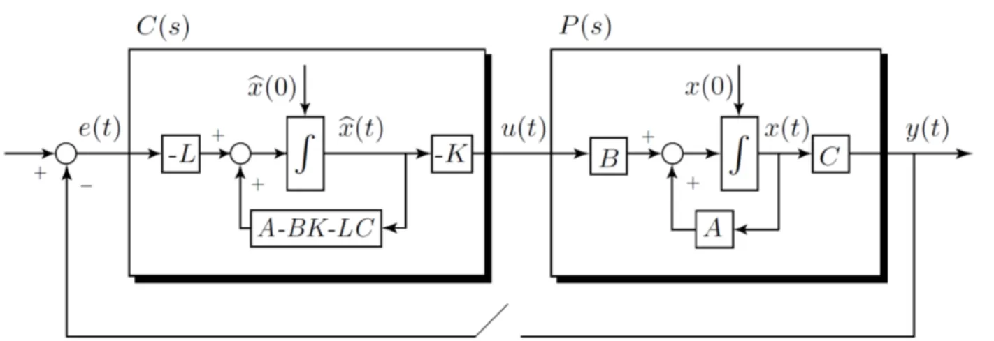
For the following explanations, I refer to Figure 1. The idea is tocopy the internal description of the plant and its dynamics, in order to predict ˆx(t). This is done by connecting two feedback loops through the observer gain L, that can be tuned for different applications. First of all, let’s define the observation error as
¯
x(t) =x(t)−x(t)ˆ ∈Rn. (11.1) The dynamics of the error are described by its derivative, namely
d
dtx(t) =¯ d
dtx(t)− d dtx(t)ˆ
=A·x(t) +B·u(t)−( ˆA·x(t) + ˆˆ B·u(t) +L·(C·x(t)−Cˆ·x(t)))ˆ
=A·x(t)¯ −L·C·x(t)¯
= (A−L·C)·x(t),¯
(11.2)
by assuming the exact duplication of the system’s dynamics, i.e. A= ˆA, B = ˆB and C = ˆC.
If the matrix A −L·C has asymptotically stable eigenvalues, the observation error will converge asymptotically to 0. The speed of convergence can betuned with the gain L.
The whole point here, is to find such a matrix with asymptotically stable eigenvalues. Since with the LQR approach we are guaranteed to have asymptotically stable eigenvalues for the matrix A−B·K, we can find similarities between the two: in fact the roles of B and C are interchanged. By converting the problem, in order to get the same role for the matrices, one gets
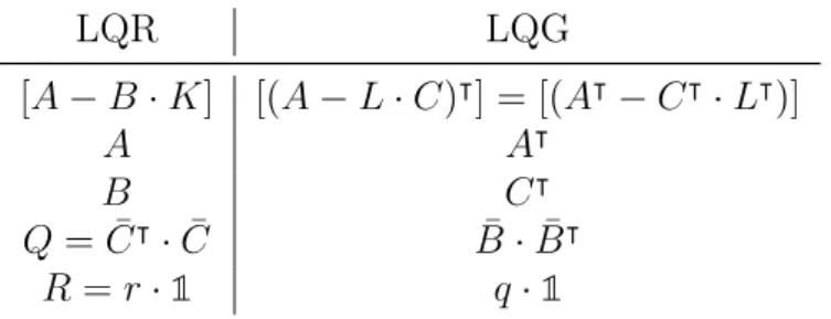
A−L·C ⇒(A−L·C)T =AT −CT ·LT (11.3) This makes the things easier: we can now, according to Table 1, approach this problem as a LQR problem with changed matrices. By plugging the new matrices into the Riccati equation, one gets
1
q ·Ψ·C|·C·Ψ−Ψ·A|−A·Ψ−B¯·B¯| = 0, (11.4) where Ψ is its solution. The matrix L is then given as
L|= 1
q ·C·Ψ. (11.5)
LQR LQG
[A−B·K] [(A−L·C)|] = [(A|−C|·L|)]
A A|
B C|
Q= ¯C|·C¯ B¯·B¯|
R =r·1 q·1
Table 1: LQG and LQR.
Figure 1: Structure of a state observer.
.
11.1.2 The LQG Controller
The LQG controller uses the LQR approach and the concept of the observer and connect the two into a unique system. Starting from the solution of the LQR problem, that contained the controller K and the observed signal ˆx(t) from the observer, one can write as learned
u(t) =−K·x(t).ˆ (11.6)
Since we have now an estimate of x(t), we can approach the problem with a normal LQR method. Let’s define
˜ x=
x(t) ˆ x(t)
. (11.7)
By connecting the observer and the plant with the gain −K one can actually analyze the open loop and the closed loop system conditions:
Open Loop Conditions
For open loop conditions, we can write the state dynamics as d
dtx(t) = ˜˜ Aopen loop·x(t) + ˜˜ Bopen loop·e(t) (11.8)
By looking at Figure 2, we can derive A˜open loop =
A −B·K 0 A−B·K −L·C
, B˜open loop =
0
−L
, C˜open loop = C 0
.
(11.9)
Closed Loop Conditions
For closed loop conditions, we can write the state dynamics as d
dtx(t) = ˜˜ Aclosed loop·x(t) + ˜˜ Bclosed loop·e(t) (11.10) and analogously it follows from Figure 2 that
A˜closed loop =
A −B·K L·C A−B ·K −L·C
, B˜closed loop =
0
−L
, C˜closed loop = C 0
.
(11.11)
If one analyzes this in the frequency domain, one gets LLQG(s) =P(s)·C(s)
=C·(s·1−A))−1·B
| {z }
P(s)
·K·(s·1−(A−B ·K−L·C))−1·L
| {z }
C(s)
(11.12) and
TLQG(s) =LLQG(s)·(1+LLQG(s))−1. (11.13) Remark.
• If the LQ regulator and the observer are stable, then so is the LQG closed loop.
• If the LQ regulator and the observer are robust, nothing can be said about the robustness of the LQG closed loop. This means that we don’t habe guarantee on robustness and it must be investigated a posteriori.
11.1.3 Kochrezept
(I) Find K: Solve a standard LQR problem with
{A, B, Q= ¯CT ·C, R}¯ (11.14) (II) Find L: Solve a standard LQR problem with
{AT, CT, Q= ¯B·B, R¯ =qT, R=q·1} (11.15) (III) Use theMatlab command
K=lqr(A,B,C_tilde’*C_tilde,r*eye(m,m)),L=lqr(A’,C’,B_bar*B_bar’,q*eye(p,p))’.
Remark. It must hold
• {A, C} completely observable
• {A,B}¯ completely controllable.
Figure 2: Structure of LQG controller.
. 11.1.4 Examples
Example 1. The dynamics of a system are given as
˙
x1(t) = x2(t)
˙
x2(t) = u(t) y(t) = x1(t).
You want to design a state observer. The observer should use the measurements for y(t) and u(t) in order to estimate the state variables ˆx(t)∼x(t).
(a) Which dimension has the observer matrixL? Draw the signal diagram of such an observer.
(b) Compute the observer matrix Lfor q = 1.
(c) You have already computed a state feedback matrix K = 1 1
for the system above.
What is the complete transfer function of the controller C(s)? UseL= √
2 1
.
Solution.
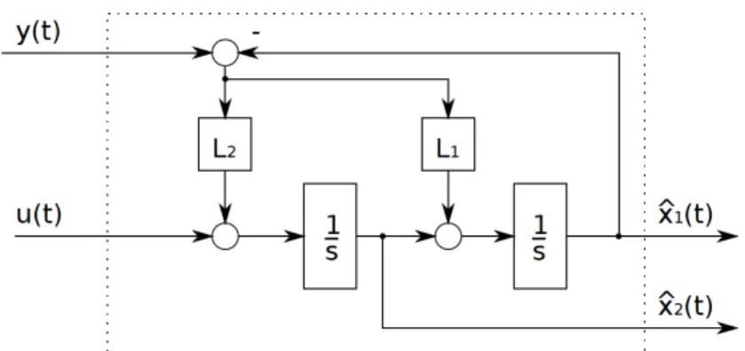
(a) Since C is a 1×2 matrix andL·Cis of the same dimensions of A, 2×2 matrix, L is a 2×1 matrix, i.e.
L= L1
L2
.
By adapting the general structure of an observer one gets Figure 3.
Figure 3: Structure of the state observer.
. (b) First of all let’s read the system matrices:
A= 0 1
0 0
B = 0
1 C = 1 0 D= 0.
Plugging these matrices into the Riccati equation one gets:
1
q ·Ψ·CT ·C·Ψ−Ψ·AT −A·Ψ−B·BT = 0 Ψ·
1 0
· 1 0
·Ψ−Ψ· 0 1
0 0
− 0 0
1 0
·Ψ− 1
0
· 0 1
= 0 0
0 0 ψ12 ψ1·ψ2
ψ1·ψ2 ψ22
−
2ψ2 ψ3
ψ3 0
− 0 0
0 1
= 0 0
0 0
.
The matrix Ψ is symmetric and positive definite and with these informations we can compute its elements:
• From the last term of the equation one gets
ψ22 = 1 ⇒ψ2 =±1.
• By plugging this into the first equation one gets ψ1 = ±√
2. Because the positive definite condition, one getsψ1 =√
2, ψ2 = 1.
• Because of the form ofC we don’t care about ψ3.
From these calculations it follows LT = 1
q ·C·Ψ
= 1
1 · 1 0
· √
2 1
1 ∗
= √
2 1 , and so
L= √
2 1
.
(c) As it is shown in the theory, the formula to calculate the controller’s transfer function reads
C(s) =K ·(s·1−(A−B·K −L·C))−1·L.
By plugging in the found matrices one gets (A−B·K −L·C) =
0 1 0 0
− 0
1
· 1 1
− √
2 1
· 1 0
= 0 1
0 0
− 0 0
1 1
− √
2 0
1 0
= −√
2 1
−2 −1
.
It follows
(s·1−(A−B·K−L·C))−1 =
s+√
2 −1 2 s+ 1
−1
= 1
(s+√
2)·(s+ 1) + 2·
s+ 1 1
−2 s+√ 2
. By plugging this into the formula one gets
C(s) =K·(s·1−(A−B·K−L·C))−1 ·L
= 1 1
· 1
(s+√
2)·(s+ 1) + 2·
s+ 1 1
−2 s+√ 2
· √
2 1
= 1
(s+√
2)·(s+ 1) + 2 · s−1 s+ 1 +√ 2
· √
2 1
= 1
(s+√
2)·(s+ 1) + 2 ·(√
2s−√
2 +s+ 1 +√ 2)
= (√
2 + 1)s+ 1 (s+√
2)·(s+ 1) + 2.
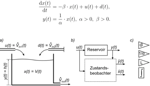
Example 2. You are working for your semester thesis at a project which includes a water reservoir. Your task is to determine the disturbance d(t) that acts on the reservoir. Figure ??
shows the situation. The only state of the system is the water volumex(t) =V(t). The volume flows in the reservoir Vin∗(t) are the known system input u(t) and the unknown disturbance d(t) > 0. The volume flow of the system is assumed to be only dependend on the water volume, i.e.
Vout∗ (t) = −β·x(t).
The system output y(t) is the water level h(t). The model of this reservoir reads dx(t)
dt =−β·x(t) +u(t) +d(t), y(t) = 1
α ·x(t), α >0, β >0.
(11.16)
Figure 4: a) Drawing of the reservoir; b) Inputs and Outputs of the observer; c) Blocks for signal flow diagram.
.
The goal is to determined(t). Your supervisor has already tried to solve the model equations for d(t): he couldn’t determine the change in volume dx(t)dt with enough precision. Hence, you want to solve this problem with a state observer.
(a) Draw the signal flow diagram of such a state observer. Use the blocks of Figure ??c).
(b) The state feedback matrix Lis in this case some scalar value. Which value can L be, in order to get an asymptotically stable state observer?
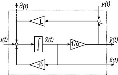
(c) Introduce a new signal ˆd(t) in the state observer. This should approximate the real disturbance d(t).
(d) Find the state space description of the observer with inputs u(t) and y(t) and output d(t).ˆ
Solution.
(a) The signal flow diagram can be seen in Figure 5.
Figure 5: Signal flow diagram of the state observer.
.
(b) The stability of the ovserver depends on the eigenvalues of A−L·C. In this case, since A−L·C is a scalar,
A−L·C < 0 should hold. This leads to
L > A C . With the given informations it follows
L >−β α.
(c) The dashed line in Figure 5 represents the new output ˆd(t). The integrator in Figure 5 has now 3 inputs. The arrow from downwards from the reservoir isVout∗ (t), the arrow from left is the input flowu(t) =Vin1∗ (t). If we simulate the system without the dashed arrow, there is a deviation between the measuredy(t) and the simulated ˆy(t). This results from the extra inflow d(t) =Vin∗(t), which is not considered in the simulation.
(d) The new state-space description reads dˆx(t)
dt =
−β− L α
·x(t) + (1)ˆ ·u(t) + (L)·y(t) d(t) =ˆ
−L α
·x(t) + (0)ˆ ·u(t) + (L)·y(t).