Evaluation of the impact of anthropogenic heat emissions generated from road transportation and power plants on the UHI intensity of Singapore

(1)

Research Collection

Report

Evaluation of the impact of anthropogenic heat emissions

generated from road transportation and power plants on the UHI intensity of Singapore

Author(s):

Singh, Vivek Kumar; Acero, Juan A.; Martilli, Alberto Publication Date:

2020-11-23 Permanent Link:

https://doi.org/10.3929/ethz-b-000452434

Rights / License:

In Copyright - Non-Commercial Use Permitted

This page was generated automatically upon download from the ETH Zurich Research Collection. For more information please consult the Terms of use.

(2)

DELIVERABLE TECHNICAL REPORT

Version 23/11/2020

D 1.2.1.3 – Evaluation of the impact of anthropogenic heat emissions generated from road transportation and power

plants on the UHI intensity of Singapore.

Project ID NRF2019VSG-UCD-001

Project Title Cooling Singapore 1.5:

Virtual Singapore Urban Climate Design

Deliverable ID

D1.2.1.3 – Evaluation of the impact of

anthropogenic heat emissions generated from road transportation and power plants on the UHI intensity of Singapore

Authors Vivek Kumar Singh, Juan Angel Acero,

Alberto Martilli

Contributors Omer Mughal, Jordan Ivanchev, David Kayanan DOI (ETH Collection) 10.3929/ethz-b-000452434

Date of Report 23/11/2020

Version Date Modifications Reviewed by

1 15/11/2020 Original Leslie Norford, Jimeno Fonseca

(3)

Abstract

This work studies the potential impact of road transport and power plants on the urban climate of Singapore. The study furthermore enhances the representation of anthropogenic heat fluxes in the Weather Research and Forecasting (WRF) model coupled with the Building Energy Model (BEM). To enhance WRF -BEM model's capacity, we have incorporated the hourly heat emission profile of road traffic and power plants and named it “Improved WRF-BEM”. This version was tested over April 2016, a period usually with high Urban Heat Island Intensity (UHII) in Singapore. The evaluation of the model performance was carried out over 17 observation stations in Singapore. The diurnal profile of hourly average temperature was close to the observation data with RMSE lower than 2°C (overall time period) for all stations. The maximum local impact of road traffic and power plant was observed during the morning and early evening respectively, reaching a maximum of 1.1 °C and 0.5 °C in each case. The highest UHII was noticed during the early morning. At hour 8:00, spatial mean UHII throughout Singapore was 1.9 °C during April 2016, reaching a maximum value of 5.2°C. As a mitigation approach, all the current vehicles were replaced by electric vehicles and additional anthropogenic heat emission was considered from the corresponding power plants. We analyzed two technology scenarios related to urban road traffic. The first scenario replaces the whole vehicle fleet of Singapore for electric vehicles. The second scenario replaces the fleet for autonomous vehicles. We found that electric vehicles lead to a drop in air temperature of more than 0.2°C in 37% of the road traffic areas, reaching a maximum reduction of 0.9°C during the early morning (8:00). Similar results are obtained for the autonomous vehicles although the spatial distribution of the impact is different. When considering the case where power plants increase their heat emission due to the production of energy for the electric vehicles scenario, our results showed slightly lower benefits on air temperature. Although maximum impact remains the same (-0.9°C), only 26.7% of the road traffic area reduces more than 0.2°C. Additionally, some areas surrounding the power plants, can expect a minor increase on air temperature.

(4)

Table of Contents

Abstract ... 2

1. Introduction ... 4

2. Study Area ... 5

3. Method ... 6

3.1. WRF-BEM model ... 7

3.3. Power Plant Model ... 12

3.4. Framework for simulation ... 12

3.6 Performance indicators for model validation and UHI estimation ... 18

4. Results and Discussion ... 19

4.1 Model performance analysis ... 20

4.2 Impact of current road traffic and power plants on air temperature ... 23

4.3. Analysis of the UHI intensity ... 27

4.4. Mitigation scenario ... 29

5. Conclusion ... 31

6. Limitation and future work ... 32

7. References ... 33

(5)

1. Introduction

Urban weather modeling has become essential to study the impact of urban warming on the growing megacities of the world. To understand urban meteorology and its adverse impact on the urban environment, many researchers employ weather models. A relevant contributor towards high temperature in urban areas is the release of anthropogenic heat from buildings, transportation, power plants, industry, household activities, and others. In this context, the increase of world population is increasing energy demand (Key World Energy Statistics, 2015), which results in higher anthropogenic heat emissions associated to the energy consumption.

Studies such as Zhang et al., (2013) provide evidence that energy consumption could lead to 1

°C increase in temperature during winter in mid and high latitudes of North America and Eurasia. Similar study carried out by Ichinose et al., (1999) over Tokyo found that the anthropogenic heat emission reaches 1590 W/m²in winter, due to high electricity consumption for household and industial purposes, which further increase the air temperature by 2.5 °C. The potential impact of anthropogenic heat in urban areas can be noticed in different climatic seasons and thoughout the day since it affects wind speed, reduces boundary layer stability and enhances vertical mixing.

To understand the impact of anthropognenic heat on urban climate, scientists are using numerical models. One of these is the Weather Research and Forecasting model (WRF). WRF is a community-based numerical model used for weather research and operational forecasting (Skamarock et al., 2008). Modeling urban meteorology in urban areas requires a precise definition of urban morphology. These include land use pattern, building height information, and thermal and optical characteristics of the urban materials; therefore, in recent years, the WRF model has been improved with coupled models of the urban canopy. These developments in WRF have significantly improved the representation of the surface energy budget; therefore, it can be used in studies such as the Urban Heat Island (UHI) phenomenon (Bhati and Mohan, 2016); thermal comfort (Watkins et al., 2007); air pollution (Liao et al., 2014); heatwave (Porfiriev, 2014) and many more.

Two urban canopy models have been implemented in WRF. The first is the Single Layer Urban Canopy Model (WRF-SLUCM) (Kusaka et al., 2001; Kusaka et al., 2004). The WRF-SLUCM uses a simplified urban geometry to estimate shadowing of building, reflection or trapping of shortwave and longwave radiation, wind profile in the canopy layer, and multi-layer heat transfer within roof, wall, and road (Kusaka et al., 2004; Tewari et al., 2007). The WRF- SLUCM model has been used in many urban environmental issues such as UHI (Mohan &

Bhati, 2011; Mills et al., 2008; Peron, De Maria et al. 2015; Wang & Akbari, 2016; Yang &

Chen, 2016), air pollution (Liao et al., 2014; Mohan & Gupta, 2018; Misenis, Hu et al., 2006;

Upadhyay et al., 2018), and heavy precipitation (Yan et al., 2016; Chawla et al., 2018; Rutledge

& Hobbs, 1984; Reshmi Mohan et al., 2018), and many more. The second urban canopy model is the Multi-Layer Building Effect Parameterization (BEP) developed by Martilli et al. (2002).

WRF-BEP examines the impact of urban buildings on airflow. It considers building size, street width and building height variability. In BEP, building induced heat and momentum fluxes are considered in the whole urban canopy layer (Martilli et al., 2002; Liao et al., 2014). Some of the SLUCM features such as shadowing effect, trapping of shortwave and longwave radiation

(6)

are also included in BEP. A modified version of BEP model includes a Multi-Layer Building Energy (BEM) developed by Salamanca et al., (2010). Coupling BEP-BEM (BEM from now on) with WRF allows air conditioner use in summer for cooling and in winter for heating to estimate the total building consumption and anthropogenic heat fluxes emitted by these, which can have a relevant impact on urban meteorology at the city level. WRF-BEM model has been evaluated and used for studies such as air quality, UHI, regional climate change, and many more. Studies such as (Molnár et al., 2019; Labedens et al., 2019; Ribeiro et al., 2021; Xu et al., 2018; Yu & Miao, 2019) were conducted using the WRF-BEM model to investigate the impact of urbanization on surface metrological variables such as temperature, relative humidity, and planetary boundary layer structure.

In the present study, an improved WRF-BEM model has been used to investigate the impact of road traffic and power plants on the urban climate of the Singapore region. We have used the land-use data of Mughal et al., (2019) to define surface properties and boundary conditions.

1.2. Objective

The main objective of this study is to estimate the potential impact of road transport and power plants on the urban climate of Singapore.

The objective can be sub-divided into 5 sub-objectives as follows:

(i) Expand WRF-BEM model to incorporate third-party hourly profiles of anthropogenic heat emissions due to road transport and power plants.

(ii) Verify the new expansion of the WRF-BEM against measured climatic variables.

(iii) Evaluate the UHI intensity with the expanded WRF-BEM (including an urban canopy model and different anthropogenic heat sources).

(iv) Evaluate the impact of current anthropogenic heat emissions from road transport and power plants on the air temperature of Singapore.

(v) Evaluate the impact of anthropogenic heat emissions from future road transportation scenarios on the air temperature of Singapore.

The scope of the study is divided into different sections. Section 2 describes the study area.

Detail explanations of WRF, WRF-BEM model, road traffic model, and power plant model and the procedure of inclusion of 24-hourly emission profiles from the road traffic model and power plant model into the into WRF-BEM are described in section 3. Section 4 (result and discussion) is related to the improvement of the WRF-BEM model with the inclusion of different anthropogenic heat sources and overall impact on the UHI phenomenon over the Singapore region. Section 5 highlights the achievement of the study. Section 6 and 7 describe the conclusions, limitations and planned future work.

2. Study Area

Singapore is an island located at 1°18'52.79" N and 103°50'43.47" E in Southeast Asia.

Geographically, it is surrounded by Malaysia and Indonesia and has a total area of 693 square

(7)

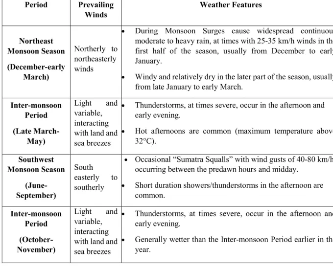
km with a 193 km coastline. Due to the high urbanized area, the country has a population of more than 5 million and has a population density of 7800 people per squarekm. The Singapore climate is hot, humid, and quite rainy throughout the year. It is characterized by two Monsoon seasons, separated by two Inter-Monsoon periods. North-East Monsoon covers December to early March and South-West Monsoon covers June to September. The two Inter-Monsoon periods are in late March-May and October-November. April is the warmest month, and November is the wettest month of the year in Singapore. Table 1 describes the Monsoon periods as well as the Inter-Monsoon periods over Singapore region.

Table 1. Description of Monsoon and Inter-Monsoon periods in Singapore Period Prevailing

Winds

Weather Features

Northeast Monsoon Season (December-early

March)

Northerly to northeasterly winds

 During Monsoon Surges cause widespread continuous moderate to heavy rain, at times with 25-35 km/h winds in the first half of the season, usually from December to early January.

 Windy and relatively dry in the later part of the season, usually from late January to early March.

Inter-monsoon Period (Late March-

May)

Light and variable, interacting with land and sea breezes

 Thunderstorms, at times severe, occur in the afternoon and early evening.

 Hot afternoons are common (maximum temperature above 32°C).

Southwest Monsoon Season

(June- September)

South easterly to southerly

 Occasional “Sumatra Squalls” with wind gusts of 40-80 km/h occurring between the predawn hours and midday.

 Short duration showers/thunderstorms in the afternoon are common.

Inter-monsoon Period (October- November)

Light and variable, interacting with land and sea breezes

 Thunderstorms, at times severe, occur in the afternoon and early evening.

 Generally wetter than the Inter-monsoon Period earlier in the year.

Currently, the study focuses on April 2016 (i.e. Inter-Monsoon period), when the UHI phenomena is enhanced in Singapore (Li et al., 2013). Additionally in April 2016 a heat wave occurred in Singapore with daily maximum temperature reaching 36°C.

3. Method

In this section we describe the different models (climatic, road traffic, power plants) used to perform the calculations (Section 3.1, 3.2, 3.3). In Section 3.4 we describe the modification required to attain the objectives of the work. The simulations of the scenarios carried out are described in Section 3.5. Finally, Section 3.6 includes the data used to validate the climate modelling framework as well as the indicators used for that aim.

(8)

3.1. WRF-BEM model

WRF is a community-based numerical model coupled with the NOAH Land Surface Model (NOAH-LSM) and with the Building Energy Model (BEM), embedded in Multi-Layer BEP developed by (Martilli et al., 2002). The primary function of coupling BEM with the WRF model is to improve the physics of the lower part of the planetary boundary layer (PBL) such as surface fluxes and temperature (surface sensible and latent heat flux and surface skin temperature). The coupling is carried out on an urban grid (for grid cells classified as LCZs) with urban fraction parameters representing the total percentage cover of impervious surface present in a grid cell (Salamanca et al., 2018). NOAH-LSM provides total surface fluxes from the vegetated surface, whereas UCM provides total surface fluxes from the impervious surface.

Therefore, the average of both sensible heat flux is considered as a total sensible heat flux per grid cell. Similarly, latent heat flux, upward longwave radiation flux, albedo, emissivity, and surface skin temperature (Salamanca et al., 2018) are also calculated.

3.1.1. Simulation period and model configuration

The complete month of April 2016 has been considered as the period of study. The simulation starts from 31 March 2016 UTC to 02 May 2016. We have used five nested domains of 24.3 km, 8.1 km, 2.7 km, 0.9 km, and 0.3 km horizontal grid spacing of outer (Domain 1), middle (Domain 2), and inner (Domain 3, 4, and 5) domains in the WRF model configuration as shown in Figure 1. Domain 1 contains a total of 76 x 76 grid points; Domain 2, 79 x 91 grid points;

Domain 3, 112 x 112 grid points; Domain 4 112 x 112 grid points; and Domain 5 211 x 130 grid points. The same configuration as describe by (Mughal, 2020) is used in all the simulations of scenarios, which are presented (Section 3.5) and discussed (Section 4) in this report.

In the WRF model, vertical height has been defined in terms of pressure level. Therefore there are a total of 51 vertical levels which are as follows: 1.0000, 0.9987, 0.9975, 0.9962, 0.9950, 0.9937, 0.9923, 0.9908, 0.9891, 0.9873, 0.9853, 0.9831, 0.9806, 0.9779, 0.9749, 0.9717, 0.9681, 0.9642, 0.9598, 0.9550, 0.9498, 0.9440, 0.9377, 0.9307, 0.9230, 0.9145, 0.9052, 0.8950, 0.8838, 0.8714, 0.8578, 0.8428, 0.8263, 0.8082, 0.7883, 0.7663, 0.7422, 0.7157, 0.6865, 0.6544, 0.6191, 0.5802, 0.5375, 0.4905, 0.4388, 0.3819, 0.3194, 0.2506, 0.1749, 0.0916, 0.0000 mbar. Global Data Assimilation System (GDAS) 6‐hourly final analysis (GDAS/FNL) data of resolution 0.25° X 0.25° has been used to construct the model's initial and boundary conditions. The model time step for the coarsest grid has been set to 81 seconds and it is reduced with a ratio of three for each nest. Model outputs are selected to be stored as an average hourly value of the meteorological variables, such as the air temperature at the lowest model level which is approximately 10 m thick. The model simulation starts with coordinated universal time (UTC) to analyze the data. We first use the nearest grid interpolation technique for data extraction, thereby adding +8 hours to analyze the model data with the observation data at local standard time (LST). Statistical and spatial analysis was carried out removing the first 16 hours as a spin-up period, and thereby. The hourly output data was compared to the hourly average temperature data provided by the National Environmental Agency (NEA) of Singapore (see Section 3.6).

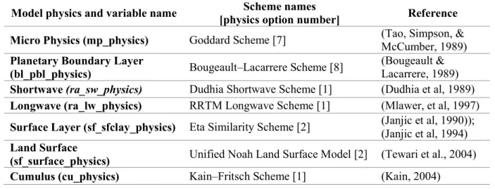
Table 2 explains the different physical parameterization schemes used in the WRF model as describe in Mughal, (2020). For the microphysics considering variations in hydrometeors and formation of clouds Goddard scheme is used . Bougeault–Lacarrere scheme is used to describe

(9)

the PBL and the atmospheric stability. Eta similarity surface layer scheme with Dudhia Shortwave and RRTM (Rapid Radiative Transfer Model) Longwave schemes are used for calculation of sensible heat flux, latent heat flux and downward solar radiation. For the vegetated area, the unificed Noah land surface model is used to calculate sensible heat flux and latent heat flux. Finally, Kain-Fritsch Scheme is used for cloud fraction and cloud cover over the simulated domain.

Figure 1: Nested domain of WRF model with horizontal grid spacing of D1: 24.3 km, D2: 8.1 km, D3: 2.7 km, D4: 0.9 km and D5: 0.3 km. Singapore region [shaded region] is shown in domain 5 with magenta color

Table 2: Different type of physical parameterization scheme used in the WRF Model

Model physics and variable name Scheme names

[physics option number] Reference Micro Physics (mp_physics) Goddard Scheme [7] (Tao, Simpson, &

McCumber, 1989) Planetary Boundary Layer

(bl_pbl_physics) Bougeault–Lacarrere Scheme [8] (Bougeault &

Lacarrere, 1989) Shortwave (ra_sw_physics) Dudhia Shortwave Scheme [1] (Dudhia et al, 1989) Longwave (ra_lw_physics) RRTM Longwave Scheme [1] (Mlawer, et al, 1997) Surface Layer (sf_sfclay_physics) Eta Similarity Scheme [2] (Janjic et al, 1990));

(Janjic et al, 1994) Land Surface

(sf_surface_physics) Unified Noah Land Surface Model [2] (Tewari et al., 2004) Cumulus (cu_physics) Kain–Fritsch Scheme [1] (Kain, 2004)

3.1.2 Land use land cover categories and urban parameterization in WRF-BEM

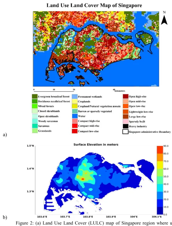
Default IGBP-MODIS 20 land use categories available in the WRF model have been considered as a representation of land use land cover in all domains except in domain 5 where we have provided an updated representation of Land Use Land Cover (LULC) in the model input (Figure 2(a)). The urban area has been characterized into10 local climate zone categories (namely as LCZ1: Compact high rise; LCZ2: Compact midrise; LCZ3: Compact low-rise;

(10)

LCZ4: Open high-rise; LCZ5: Open midrise; LCZ6: Open low-rise; LCZ7: Lightweight low- rise; LCZ8: Large low-rise; LCZ 9: Sparsely built; LCZ10: Heavy industry) derived from Landsat 8 images and high-resolution building height data (Mughal, 2020).

a)

b)

Figure 2: (a) Land Use Land Cover (LULC) map of Singapore region where urban area is classifiedbased on Local Climate Zones (LCZs) and (b) surface elevation in meter over Singapore region using Shuttle Radar Topography Mission Digital Terrain Elevation Data (SRTM DTED) 30s data

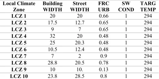
Some of the essential urban parameters mentioned in Table 3 and Table 4 are used to represent LCZs in the WRF model. Table 3 describes the urban parameters in terms of LCZ built-up type and its associated mean building height, roof width, road width, and urban fraction. Table 3 also provides information related to the use of air conditioners. Table 4 describes average

(11)

height (in meters) of each LCZ in meter, the height distribution of each LCZ building and percentage cover of each building height distribution.

Table 3: Different type of urban parameter used in WRF-BEM Model Local Climate

Zone

Building WIDTH

Street WIDTH

FRC URB

SW COND

TARG TEMP

LCZ 1 20 20 0.66 1 294

LCZ 2 17.5 12.7 0.65 1 294

LCZ 3 9 7 0.65 1 294

LCZ 4 32 20 0.48 1 294

LCZ 5 25 20.3 0.48 1 294

LCZ 6 10.5 12.4 0.48 1 294

LCZ 7 7 2 0.9 1 294

LCZ 8 28.8 20.5 0.78 1 294

LCZ 9 10 10. 0.13 1 294

LCZ 10 23.8 28.5 0.8 1 294

where Building WIDTH is noted as roof width in meter, Street WIDTH is denoted as road width in meter, FRC URB is denoted as fraction of urban landscape (fraction: 0 to 1), SW COND is denoted as air conditioning switch on and TARG TEMP is denoted as target temperature of air conditioner system in Kelvin. A value of 21ºC (294ºK) was set for building indoor temperature, taken as a reference from Singaporean Agencies brenchmarks.

Table 4: LCZs building height distribution used in WRF-BEM

LCZ Average

Height (m)

Height Distribution

(m)

Percentage (%)

1 42.3

25 25

40 50

60 25

2 15.8

10 25

20 50

30 25

3 6.7 5 75

10 25

4 38

25 25

40 50

50 25

5 14

10 25

20 50

30 25

6 5.9 5 75

10 25

7 6.5 5 100

8 6.5 5 75

10 25

9 5.6 5 75

10 25

10 7.6 5 75

10 25

(12)

3.2. City MoS Model

In order to estimate heat emissions from road traffic we have utilized an agent-based road traffic simulation model called CityMoS (Ivanchev et al, 2020). In the work of Ivanchev et al (2020), the model is calibrated and validated using real road traffic data of the city-state of Singapore. The model was used to simulate three types of road traffic emission scenarios: Base case emission scenario (BS), electric vehicle emission scenario (EV), and autonomous emission scenario (AE).

In the BS scenario, the road traffic patterns throughout the day are represent the current state of the Singapore road transport system and the vehicle population is mostly composed of vehicles using diesel or petrol. In the EV scenario, all vehicles are replaced by electric vehicles, however the routes of the vehicle population remain unchanged. Finally, in the AE scenario, all vehicles are both electric and autonomous. This implies that the road traffic patterns and capacities of the road network are adjusted and thus the transport system dynamics is different.

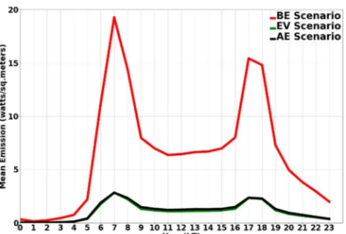
In these three scenarios, the anthropogenic heat (AH) emissions are considered to be released in the lowest model level. Figure 3 describes the diurnal profile of monthly mean emission of the road traffic scenarios from the CityMoS model.

Figure 3: Diurnal profile of emissions profile from different road traffic scenarios where the red line indicates base case scenario (BS), the black line indicates an electric vehicle scenario (EV), and the green line indicates an autonomous scenario (AE).

It can be noted from Figure 3 that, in all scenarios, the maximum emission released from road traffic is during the early morning and late evening of the day, that correspond to rush hours.

There is a very slight variation in emission profiles between EV and AE scenarios. The CityMoS model estimates that emissions from EV and AE scenarios lie between 0 and 5 W/m². In contrast, the BS scenario shows much higher values with maxima emission ranges between 0 to 20 W/m².

(13)

3.3. Power Plant Model

According to Kayanan, Fonseca, & Norford (2020), the power plant dispatch model has been used to calculate total anthropogenic heat release from power plants over the Singapore region.

The dispatch model provides data from two different scenarios: the power plant base case (PBS scenario) and power plant electric vehicle (PEV scenario) described in Section 3.5.

In the PBS scenario, emissions are calculated based on total fuel consumed to produce electricity for the whole of Singapore. In contrast, in the PEV scenario, electricity consumption increases due to the complete electrification of road transportation, i.e., electric vehicles. All the emissions are released as per the height of the stack. Figure 4 describes the diurnal profile of monthly mean emission of the two scenarios considered in the power plant dispatch model.

Figure 4: Diurnal profile of emissions profile from different power plant scenarios; the red line indicates the Power Base case Scenario (PBS), and the green line indicates the Power Electric Vehicle scenario (PEV).

It can be noted from Figure 4 that, in all scenarios, the maximum emission released from power plant is during the early morning and late evening of the day. There is a slight variation in emission profiles between PBS and PEV scenarios. The power plant model estimates +7.6 % higher emissions in PEV in comparison to PBS scenarios, because of additional electricity demand for electric vehicle charging (Kayanan et al., 2020). In can be noted from Figure 4 that between 0800 hour to 1100 hour, PEV emission lies between 2500 to 2750 Watt per sq. meter whereas in case of PBS scenario, emission lies between 2250 to 2500 Watt per sq. meter.

3.4. Framework for simulation

To achieve the objective of the study, we have modified two input variables in the WRF preprocessing system: the LU_INDEX variable, which represents the LCZ distribution over the Singapore region, and the HGT_M variable, which represent the surface elevation from the mean sea level as described in Figure 2(a-b). A modification related to land use land cover representation in the WRFV3 part of the WRF model is also carried out. Complete details related to the role of LCZs and code modification are described in the technical report Mughal et al. (2020). Figure 5 describe the complete workflow diagram for the WRF-BEM model.

(14)

Figure 5: WRF Workflow with the integration of anthropogenic heat from road traffic and power plant.

3.4.1 Required modification to include anthropogenic heat emissions from road traffic and power plants in the WRF-BEM model

Below is the description of the modification that was done in the WRF-BEM code to include anthropogenic heat emission from road traffic and power plants in the model. Below is the list of modules to be modified,.

(i) module_physics_init.F

In the present study, we have added a 24-hourly emission file (text file) of road traffic and power plant at the finest domain 5 (210x129) grid point. Therefore, the dimension of the traffic_matrix variable in WRF to digest the mentioned road traffic emission file will require a time step=24, west_east=210 and south_north=129 (see below).

In SUBROUTINE bl_init ( … & …):

REAL, DIMENSION(Time,west_east,south_north) :: traffic_matrix REAL, DIMENSION(Time,west_east,south_north) :: power matrix

IF(SF_URBAN_PHYSICS.eq.1).OR.(SF_URBAN_PHYSICS.EQ.2).OR.(SF_URBAN_PHYSI CS.EQ.3)) THEN

CALL vivek_subroutine_traffic(traffic_matrix) CALL vivek_subroutine_power(power matrix) END IF

(15)

(ii) module_sf_noahdrv.F

REAL,DIMENSION(24,210,129)::VS_TRAFFIC REAL,DIMENSION(24,210,129)::VS_Power

SUBROUTINE vivek_subroutine_traffic (traffic_matrix)

REAL, DIMENSION (Time, west_east, south_north), INTENT (INOUT):: vivek_traffic_matrix INTEGER: ii, jj, kk, vsi, index_count

REAL, DIMENSION(27090)::AH_Hour1,AH_Hour2,AH_Hour3,AH_Hour4,AH_Hour5,&

AH_Hour6,AH_Hour7,AH_Hour8,AH_Hour9,AH_Hour10,AH_Hour11,AH_Hour12,&

AH_Hour13,AH_Hour14,AH_Hour15,AH_Hour16,AH_Hour17,AH_Hour18,&

AH_Hour19,AH_Hour20,AH_Hour21,AH_Hour22,AH_Hour23,AH_Hour24 Open(22,file='Basecase_Traffic_emission.txt',status='old')

DO vsi=1,27090

read(22,*)AH_Hour1(vsi),AH_Hour2(vsi),AH_Hour3(vsi),AH_Hour4(vsi),AH_Hour5(vsi),&

AH_Hour6(vsi),AH_Hour7(vsi),AH_Hour8(vsi),AH_Hour9(vsi),AH_Hour10(vsi),AH_Hour1 1(vsi),AH_Hour12(vsi),&AH_Hour13(vsi),AH_Hour14(vsi),AH_Hour15(vsi),AH_Hour16(vsi ),AH_Hour17(vsi),AH_Hour18(vsi),&AH_Hour19(vsi),AH_Hour20(vsi),AH_Hour21(vsi),AH _Hour22(vsi),AH_Hour23(vsi),AH_Hour24(vsi)

END DO Close (22) DO ii=1,24 index_count=1 DO jj=1,210 DO kk = 1,129 if(ii .eq. 1) then

vivek_traffic_matrix(ii,jj,kk)=AH_Hour1(index_count) VS_TRAFFIC (ii,jj,kk)=vivek_traffic_matrix(ii,jj,kk) index_count=index_count+1

else if(ii .eq. 2) then

print *,VS_TRAFFIC(ii,jj,kk) else if(ii .eq. 4) then

vivek_traffic_matrix(ii,jj,kk)=AH_Hour5(index_count) VS_TRAFFIC (ii,jj,kk)=vivek_traffic_matrix(ii,jj,kk)

(16)

index_count=index_count+1 else if(ii .eq. 6) then

vivek_traffic_matrix(ii,jj,kk)=AH_Hour7(index_count) VS_TRAFFIC(ii,jj,kk)=vivek_traffic_matrix(ii,jj,kk) index_count=index_count+1

(17)

end if END DO END DO END DO RETURN

END SUBROUTINE vivek_subroutine_traffic

The same structure of the above routine (for traffic_matrix emissions) is also embedded in the WRF model to read and include the power plants emissions in the simulations

It can be noted that the 24-hourly traffic emission data are introduced at ground (lowest level) and included in the climate calculations of WRF as follows:

b_t_bep(i,1,j)=b_t_bep(i,1,j)+VS_TRAFFIC(VS_Hour,i,j)/(dz8w(i,1,j)*rho(i,1,j)*CP*VL_BE P(I,1,J))

(18)

whereas power emission is released at specific height, therefore

b_t_bep(i,k,j)=b_t_bep(i,k,j)+VS_Power(VS_Hour,i,j)/(dz8w(i,1,j)*rho(i,1,j)*CP*VL_BEP(I, 1,J))

where k is the level of heat release in the atmosphere, b_t_bep is potential temperature in K, dz8w is denoted as vertical grid spacing in meter, rho is density of air in kg/m3, CP is specific heat capacity of air in Kj/kg, VL_BEP is fraction of air volume in air grid cell.

3.5 Simulation design

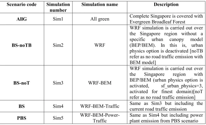
A total of eight simulations were performed to evaluate anthropogenic heat's role on the urban climate and evaluate mitigation strategies for road traffic over the Singapore region. These simulations were carried out for the month of April 2016. Table 5a describes the list of simulations and Table 5b describes mitigation strategies over Singapore region.

Table 5a: Simulations in the WRF model and their description Scenario code Simulation

number

Simulation name Description

AllG Sim1 All green Complete Singapore is covered with Evergreen Broadleaf Forest

BS-noTB Sim2 WRF

WRF simulation is carried out over the Singapore region without a specific urban canopy model (BEP/BEM). In this is, urban physics option is deactivated [noTB refer as no road traffic emission with BEM model]

BS-noT Sim3 WRF-BEM

WRF simulation is carried out over the Singapore region with BEP/BEM (urban physics option is activated, sf_urban_physics=3, activated for finest domain)[noT refer as no road traffic emission]

BS Sim4 WRF-BEM-Traffic Same as Sim3 but including the current road traffic emission

PBS Sim5 WRF-BEM-Power-

Traffic

Same as Sim4 but including power plant emission from PBS scenario

(19)

Table 5b: Mitigation scenario simulations in the WRF model and their description Scenario

code

Simulation

number Simulation name Description

EV Sim6 WRF-BEM- Traffic

[Electric]

Same as Sim4 but including the road traffic emission from EV scenario

AE Sim7 WRF-BEM- Traffic

[Autonomous]

Same as Sim4 but including the road traffic emission from AE scenario PEV Sim8 WRF-BEM-Power- Traffic

[Electric]

Same as Sim5 but including power plant emission from PEV scenario

3.6 Performance indicators for model validation and UHI estimation

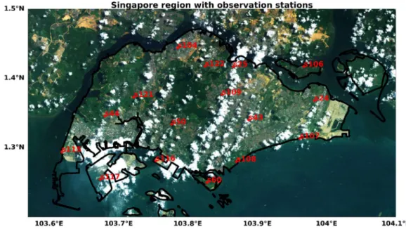
To validate the performance of model, we have used hourly average observation data of April 2016 collected from 17 observation stations. The data has been provided by the National Environmental Agency (NEA), Singapore. The observation data consist of temperature, relative humidity, and dew point temperature. In the study, we focussed on the diurnal cycle of air temperature over the Singapore region. Figure 6 shows each observation station's location with station numbers, and Table 6 describe the name, location in terms of latitude and longitude, and instrument height from mean sea level. It can be noted that some stations arelocated at the ground level , while others are located on building roofs.

Figure 6: Singapore region with station numbers indicated in red colour

In the current study, Mean Bias (MB) and Root Mean Square Error (RMSE) have been used to validate the model. Emery et al. (2001) proposed statistical benchmarks for the meteorological parameters such as temperature: Bias ± 0.5 °C and Carbonell et al. (2013) for RMSE 2.0 °C.

(20)

Let us consider and represent predicted/simulated mean and observed mean, respectively (Gunwani and Mohan, 2017), therefore:

 Bias: =

 Root Mean Square Error (RMSE): =

The predicted/simulated values were extracted from the model outputs at the closest height to one of the observation station.

Table 6: Observation station details with the height above mean sea level Station

Number

Mounted Location

Station Name Latitude [degree]

Longitude [degree]

Height above mean sea

level [m]

S102 ground Semakau Island 1.189 103.768 6

S106 ground Pulau Ubin 1.4168 103.9673 27

S107 ground East Coast Parkway 1.3134 103.9619 9

S108 ground Marina Barrage 1.2799 103.8703 15

S115 ground Tuas South 1.2938 103.6184 6

S122 ground Khatib 1.4173 103.8249 26

S24 ground Changi 1.3678 103.9826 15

S104 roof top Admiralty 1.4439 103.7854 27

S109 roof top Ang Mo Kio 1.3764 103.8492 53

S111 roof top Newton 1.3106 103.8365 115

S116 roof top Pasir Panjang 1.281 103.754 26

S117 roof top Jurong Island 1.2542 103.6741 22 S121 roof top Choa Chu Kang (South) 1.3729 103.7224 38

S43 roof top Tai Seng 1.3399 103.8878 36

S44 roof top Jurong (West) 1.3455 103.6806 84

S50 roof top Clementi 1.3337 103.7768 69

S60 roof top Sentosa Island 1.25 103.8279 37

4. Results and Discussion

The current study has been sub-divided into four sections, in which section 4.1 describes the performance of the simulations described in Table 5a. Section 4.2 describes the impact on air temperature over the Singapore region due to emission from current road traffic (BS scenario) and power plants (PBS scenario). Section 4.3 describes the levels of UHI intensity including the contribution of current AH emission sources (road traffic and power plants) (Scenario PBS). Finally, Section 4.4 describes the mitigation approach by replacing the existing vehicles with the electric vehicle (EV, AE and PEV scenarios) as mentioned in Table 5b.

P O

P O

2 1

(1/ ) ^N

( )

i

N

P O

i i







(21)

4.1 Model performance analysis

Figure 7 and Figure 8 show the diurnal profile of hourly average near-surface air temperature from different simulations mentioned in Table 5a and Table 5b compared with observation stations in Singapore.

Figure 7: Diurnal profile of hourly average air temperature on observation stations mounted at specific height from ground level (see Table 6).

(22)

Figure 8: Diurnal profile of hourly average air temperature on observation stations mounted on building roofs (see Table 6).

(23)

Figure 8 cont.: Diurnal profile of hourly average air temperature on observation stations mounted on building roofs (see Table 6).

Table 7: Statistical Analysis of WRF-BEM-Power-Traffic Simulation (PBS scenario) Station

Number

WRF-Power-Traffic RMSE [ºC] Mean Bias

S102 1.38 -1.04

S106 1.78 -0.66

S107 1.34 -0.64

S108 1.60 -0.77

S115 1.53 -0.63

S122 1.90 -0.30

S24 1.39 -0.31

S104 1.60 -0.56

S109 1.68 -0.62

S111 1.61 -0.95

S116 1.73 -1.08

S117 1.63 -0.95

S121 1.63 -0.27

S43 1.59 -0.84

S44 1.91 -1.10

S50 1.63 -0.68

S60 1.52 -0.91

From Figure 7 and Figure 8 it can be noted that all the simulations are underestimating the hourly average diurnal temperature profile with respect to the observation data. Salamanca et al., (2018), also found that the WRF-BEM model underestimates the diurnal profile of air temperature with respect to the observation data while studying the sensitivity of the land surface model. Overall the improved WRF-BEM used to simulate the building canopy with inclusion of anthropogenic emissions from road traffic and power plants (PBS scenario) produces results closer to the observation than the case of WRF-BEM simulation (BS-noT scenario). The performance of the Improved WRF-BEM (PBS scenario) for all the ground stations and elevated stations is shown in Table 7. It can be noted that the RMSE of all

(24)

observation stations was less than 2 °C (suitable threshold for deviation of a model (Carbonell et al., 2013)). and Mean Bias of all observation station was less than 0.5 (Carbonell et al. 2013;

Emery et al., 2001).

One of the possible reason for underestimating temperature profile throughout the diurnal cycle is due to diurnal mixing (Hu et al., 2010). BouLac PBL scheme is a local closure scheme which produce insufficient vertical mixing in the convective boundary layer which further results in less heat transfer from the surface to vertical layers during day (Brown, 1996). Lower cloud cover during nighttime could be one of the reason for undestimation of temperature profile (Bougeault and Lacarrere, 1989).It can be noted that station S24, overestimate temperature during afternoon whereas station S122 and S106 overestimating during nighttime or early morning. Other possible reasons are errors in the estimation of upward longwave radiation, albedo, emissivity, and surface skin temperature in the WRF model due to assumptions made in the WRF-BEM model described in Mughal et al. (2019) and Mughal et al. (2020).

The impact of heat emission from buildings, road traffic, and power plants on the air temperature profile can be noted in the early morning and afternoon/early evening hours of the day (section 4.2). Similar results were also stated for Singapore (Chow & Roth, 2006), Mexico (Jauregui, 1997), Delhi (Padmanabhamurty and Bahl, 1982), and Pune (Padmanabhamurty, 1979). Therefore, results are shown as the spatial distribution of the air temperature profile at a specific hour of the day (Figure 9, 10, 11). In the current study, we have considered the hourly average spatial distribution at hour 0:00 (midnight), hour 8:00 (early morning), and Hour 16:00 (afternoon/early evening). Spatial distribution at different hours are plotted for level 1 of the WRF model. Level 1 corresponds to the lowest model level (approximately 10 m thick).

4.2 Impact of current road traffic and power plants on air temperature

This section describes the impact of road traffic, and power plant heat emissions on air temperature over the Singapore region. Different scenarios have been considered to evaluate the impact of these anthropogenic heat emission sources:

(i) Road traffic: the temperature difference between WRF-BEM including current road traffic heat emissions (BS Scenario) and WRF-BEM simulation (BS-noT Scenario). This is described in section 4.2.1.

(ii) Power plants: the temperature difference between WRF-BEM including current road traffic and power plant heat emissions (PBS scenario) and WRF-BEM including only current road traffic (BS scenario). This is described in section 4.2.2.

4.2.1 Impact of current road traffic on air temperature

The analysis is performed only considering the grid cells that include road traffic AH emissions, i.e. with a 300 x 300 m resolution.

(25)

Figure 9 shows the spatial distribution of hourly average T2m difference between WRF-BEM including current road traffic heat emissions (BS scenario) and WRF-BEM simulation (BS- noT).

Figure 9: Spatial distribution of hourly average T2m difference between WRF-BEM- Traffic (BS scenario) and WRF-BEM (BS-noT) over Singapore region at hour 0:00 (midnight), hour 8:00 (early morning) and hour 16:00 (afternoon/early evening) with percentage of area covered

(26)

It can be noted that most of the Singapore region experiences an impact on air temperature up to 0.2 °C during midnight due to the current road traffic. During the early morning, the impact increases and the range varies mainly between 0.1 °C to 0.4 °C, whereas during the afternoon/early evening the impact decreases in most of the region to values up to 0.2 °C. It can also be noted that the maximum contribution of current road traffic reaches 1.1 °C during the early morning (in relation with the rush road traffic hour). At this time, 7.5% of area register values higher than 0.4 °C.

4.2.2 Impact of current power plants on air temperature

Figure 10 shows the contribution of power plants in Singapore to air temperature at hour 0:00, hour 8:00 and hour 16:00. It can be noted that at midnight and morning the impact (increase of air temperature) can be similar although with different spatial distribution. Most of Singapore registers increments <0.2 °C. During the afternoon/early evening impact can be higher than 0.2

°C in a relevant area (7.6%). It can also be noted that the maximum impact on air temperature reaches 0.5°C during this period of the day. One of the possible reasons for high-temperature impact during the afternoon/early evening is the extra heat added by the power plants, which may affect the convective structures' position and force additional heating of the atmosphere.

From Figure 10 we can extract that the maximum impact of power plants is in the North part of Singapore region. This represents the 0.97% of area of Singapore where values are higher than 0.4 °C during afternoon/early evening.

Table 8 summarizes the results presented in Section 4.2. It can be noted that the impact of road traffic is higher than the one of power plants over Singapore region throughout the day.

Maximum impact of road traffic is during early morning (1.1 °C) whereas for the power plants, it is in the afternoon/early evening (0.5 °C).

Table 8: Maximum contribution to air temperature from different emission sources and at different time-period of the day.

Hours

ΔTmax (°C)

Road traffic Power plant

Hour 0:00 (midnight) 0.5 0.3

Hour 8:00 (early morning) 1.1 0.2

Hour 16:00 (afternoon/early evening) 0.4 0.5

(27)

Figure 10: Spatial distribution of hourly average T2m difference between WRF- BEM-Power-Traffic (PBS scenario) minus WRF-BEM-Traffic (BE scenario) over Singapore region at hour 0:00 (midnight), hour 8:00 (early morning) and hour 16:00 (afternoon/early evening) with percentage cover

(28)

4.3. Analysis of the UHI intensity

The UHI intensity is calculated as the air temperature difference between urban land and natural land (Taha, 1997). To evaluate UHI intensity over the whole area of Singapore, we have considered the existing land cover (as described in Figure 2) including building, road traffic and power plants AH emission (PBS scenario), as well as the fully non-developed Singapore (AllG scenario).

Figure 11 shows the spatial distribution of UHI intensity at hour 0:00, hour 8:00, and hour 16:00. During midnight, it can be noted that most of the Singapore region experiences UHI intensity between 0.5 °C to 4.5 °C with a spatial mean UHI intensity of 1.8 °C. During the early morning, the UHI intensity increases and the range vary between 0.5 °C to 5.2 °C with spatial mean UHI intensity of 1.9 °C whereas the UHI intensity decreases during the afternoon/early evening and ranges between 0.5 °C to 3.5 °C with spatial mean UHI intensity of 1.1 °C. Thus, spatial maximum UHI intensity reaches 5.2 °C during the morning (as mean value during April 2016).

We can note that during hour 0:00 (midnight) and hour 8:00 (early morning), UHI intensity is highest in the southern part and some central areas of the Singapore region. During hour 0:00 (midnight), 15.2% of the area has UHI intensity more than 3.0°C and increases to 21.4% at hour 8:00 (early morning). At hour 16:00 (afternoon/early evening), area with UHI intensity higher than 3°C was only about 0.07 % of Singapore region.

(29)

Figure 11: Spatial distribution of hourly average UHI intensity including buildings, road traffic and power plants over Singapore region at hour 0:00 (midnight), hour 8:00 (early morning) and hour 16:00 (early evening) with percentage cover

(30)

4.4. Mitigation scenario

This section describes an urban heat mitigation approach by introducing an electric vehicle scenario (EV scenario) over the Singapore region. In Section 4.4.1 we compare the impact of current road traffic (BS scenario) with the impact of electric vehicles (EV scenario) and autonomous vehicles (AE scenario). In section 4.4.2 we evaluate the impact on air temperature when we include the generation of electricity in Singaporean power plants to power the electric vehicles scenario.

4.4.1. Impact of incorporating electric and autonomous vehicles on air temperature Figure 12 shows the spatial distribution of the difference on air temperature when moving from current road traffic of vehicles to electric vehicles and autonomous vehicles. Previously, in section 4.2 we saw that the maximum contribution of the current road traffic was 1.1°C and occurred during the morning (hour 8:00). With the deployment of electric and autonomous vehicles, the maximum reduction of air temperature is 0.9°C and 0.8°C respectively, also during the morning (hour 8:00). At this time, the area with a reduction higher than 0.2°C is 37% and 34.8% for the electric and autonomous scenario respectively.

During the afternoon/early evening (hour 16:00), maximum contribution of current road traffic to air temperature reaches 0.4°C (Section 4.2). When implementing an electric or autonomous scenario, we can expect a maximum reduction of 0.4°C in both cases. At this time, the area with a benefit higher than 0.2°C is much lower than during the morning period, i.e. 2.14% and 3.08% for electric and autonomous scenario respectively.

The introduction of electric and autonomous vehicles does reduce the impact of road traffic on air temperature. However, some specific and minor areas show the opposite impact, especially in the afternoon/early evening. In any case, this increase in air temperature when changing to electric vehicles is very small and is mostly associated with specific conditions/changes in the atmospheric heat fluxes. Also it is relevant to note that both for electric and autonomous vehicles, the impacts on air temperature and the spatial pattern are different since the routes taken by the vehicles in each scenario are different (i.e. different spatial distribution of AH emission).

(31)

Figure 12: Spatial distribution of hourly impact on air temperature of electric and autonomous vehicles over Singapore region at hour 8:00 (early morning) and hour 16:00 (afternoon/early evening) with percentage of area

4.4.2. Impact of electric vehicle and the generation of power on air temperature

Figure 13 shows the spatial distribution of the impact on air temperature due to the deployment of electric vehicles and the generation of the required electricity in Singapore power plants.

This represents a possible real scenario where the energy to power the electric vehicles is generated in the current power plants of Singapore.

In this case, the highest impact occurs during the morning period in agreement with results of the electric vehicles impact (Section 4.4.1). The maximum air temperature reduction reaches - 0.94°C during the early morning. At hour 8:00, the area with reduction of air temperature higher than 0.2°C is 26.7%. This value is lower than the results of the impact of deploying only electric vehicles which is in accordance with the additional AH emission in Singapore power plants considered in this mitigation measure. However, at hour 16:00h, the impact is much lower with maximum reduction of 0.3°C and only 1.37% of the area with a reduction higher than 0.2°C.

Although in most areas of Singapore there is a benefit of introducing electric vehicles (as mentioned in the previous paragraphs), small areas can experience a slight increase in air temperature. This can be due to two reasons. On one hand most of these areas are far away from the road traffic areas and thus power plants can have a greater impact. This is the case of southwestern and northern part of the Singapore where some power plants are located. On the

(32)

other hand, changes in the atmospheric circulation and microphysics of the atmosphere could be expected with the additional AH emission in power plants (required to power the electric vehicles). This issue could lead to a minor increase on air temperature in specific areas of the island.

Figure 12: Spatial distribution of hourly impact on air temperature of electric vehicles and the generation of the power required over Singapore region at hour 8:00 (early morning) and hour 16:00 (afternoon/early evening) with percentage of area

5. Conclusion

The present study focuses on improving the WRF-BEM model by incorporating anthropogenic heat emissions from road traffic and power plants. Thus, an improved estimation and evaluation of the Urban Heat Islan Intensity is presented. Similarly, we present the benefits of changing the vehicle fleet to electric, as a mitigation approach in Singapore region. We have used 24- hourly emission profile of road traffic and power plant as an input in the WRF-BEM model.

Findings reveal that after including hourly emission profiles of road traffic and power plants (so called Improved WRF-BEM model), the diurnal temperature estimation of the model fits better with the observation and have RMSE less than 2 °C for all the observation stations (Carbonell et al., 2013).

Therefore, from our study we can conclude the following points:

 Including emission of road traffic and power plants in WRF-BEM model provides a better estimation of air temperature over the Singapore region. This is more evident during the early morning and afternoon/early evening. One possible reason is high emissions in the road traffic scenarios during these periods of the day.

 For the month of April 2016, the maximum contribution of the current road traffic to air temperature is 1.1°C during the morning period (<1% of the area). At this time 7.5%

of the area of Singapore experiences an impact on air temperature higher than 0.4°C.

 Current power plant anthropogenic heat emission can have a maximum contribution of 0.5°C during the afternoon/early evening (<1% of the area). Only 0.97% of the island has an impact higher than 0.4°C

 Maximum UHI intensity during April 2016 (including building, road traffic and power plants current AH emission) is 5.2°C during the morning period (<1% of the area). Over the whole Singapore mean spatial UHI intensity reaches 1.9 °C.

(33)

 The introduction of electric vehicles (and the corresponding increase in power generated in power plants) can produce a maximum reduction on air temperature of 0.9°C (<1% of the area). Also, 26.7% of Singapore area would have a mean reduction higher than 0.2°C. Only a small part of the island (1.4%) could register reductions higher than 0.5°C during the morning.

6. Limitation and future work

The study presented in this report has some limitations. These will be addressed in coming research:

 Previous work on mesoscale modelling in Singapore ((Mughal et al., 2019) already highlighted that the BEM embedded in the WRF climatic model has limitations in the definition of diurnal antropogenic heat emissions of different building typologies. This means that in the same LCZ BEM considers the same use of air conditioners for residential and commercial buildings, which is not precise. Therefore, an improved configuration of building anthropogenic heat emissions should be estimated and spatially distributed throughout the entire urban area.

 Similarly, BEM estimations of energy consumption should be validated with real measured data (Mughal et al., 2020). This would allow fine tuning some of the parameters and physic equations inside BEM that could lead to a better quantification of the building anthropogenic heat emissions.

 The building indoor temperature was set to 21ºC, taken as a reference from Singaporean Agencies. This might be too low and not realistic and thus overestimate the energy consumption of buildings in Singapore.

 The building height distribution is based on the LCZ classification, and thus based on the model resolution a specific height is consider for each LCZ class.

 Lack of data of measured turbulent heat fluxes in the surface layer limits the validation of the model. These measurements in the inertial sub-layer represent homogeneous turbulence values resulting from the interaction of the urban canopy layer and the regional climate conditions.

 Estimation of UHI intensity for Singapore (Section 4.3) remains incomplete since a source of anthropogenic heat emissions has not been considered. Although these emissions of heat are mostly located in a specific area of Singapore (south west), they are also relevant and could further increase the urban air temperature in Singapore.

The future work will be focused in overcoming the limitations mentioned. Together with experts in the building energy field we will undertake a validation of the building energy consumption of BEM and improve/validate the estimation of the impact of the building anthropogenic heat emissions in the UHI intensity of Singapore. Availability and access to turbulent heat fluxes in Singapore would further improve the reliability of the estimations and would allow a sensitivity analysis of different surface layer and radiation schemes available in WRF. In any case the model performance in the PBLwill be analysed with daily radiosoundings of air temperature and wind.

(34)

7. References

Bhati, S., Mohan, M., 2016. WRF model evaluation for the urban heat island assessment under varying land use/land cover and reference site conditions. Theor. Appl.

Climatol. 126, 385–400. https://doi.org/10.1007/s00704-015-1589-5

Bougeault, P., Lacarrere, P., 1989. Parameterization of Orography-Induced Turbulence in a Mesobeta-Scale Model 117, 1872–1890. https://doi.org/10.1175/1520-

0493(1989)117<1872:POOITI>2.0.CO;2

Carbonell, L.T., Mastrapa, G.C., Rodriguez, Y.F., Escudero, L.A., Gacita, M.S., Morlot, A.B., Montejo, I.B., Ruiz, E.M., Rivas, S.P., 2013. Assessment of the Weather Research and Forecasting model implementation in Cuba addressed to diagnostic air quality modeling. Atmospheric Pollut. Res. 4, 64–74.

https://doi.org/10.5094/APR.2013.007

Chawla, I., Osuri, K.K., Mujumdar, P.P., Niyogi, D., 2018. Assessment of the Weather Research and Forecasting (WRF) model for simulation of extreme rainfall events in the upper Ganga Basin. Hydrol. Earth Syst. Sci. 22, 1095–1117.

https://doi.org/10.5194/hess-22-1095-2018

Chow, W.T.L., Roth, M., 2006. Temporal dynamics of the urban heat island o Singapore. Int.

J. Climatol. 26, 2243–2260. https://doi.org/10.1002/joc

Dudhia, J., 1989. Numerical Study of Convection Observed during the Winter Monsoon Experiment Using a Mesoscale Two-Dimensional Model VOL. 46, NO. 20, 3077–

3107. https://doi.org/10.1175/1520-0469(1989)046<3077:NSOCOD>2.0.CO;2 Emery, C., Tai, E., Yarwood, G., 2001. Enhanced Meteorological Modeling And

Performance Evaluation For Two Texas Ozone Episodes 235.

Gunwani, P., Mohan, M., 2017. Sensitivity of WRF model estimates to various PBL parameterizations in different climatic zones over India. Atmospheric Res. 194, 43–

65. https://doi.org/10.1016/j.atmosres.2017.04.026

Hu, X.-M., Nielsen-Gammon, J.W., Zhang, F., 2010. Evaluation of Three Planetary

Boundary Layer Schemes in the WRF Model. J. Appl. Meteorol. Climatol. 49, 1831–

1844. https://doi.org/10.1175/2010JAMC2432.1

Ichinose, T., Shimodozono, K., Hanaki, K., 1999. Impact of anthropogenic heat on urban climate in Tokyo. Atmos. Environ. 33, 3897–3909. https://doi.org/10.1016/S1352- 2310(99)00132-6

Ivanchev, J., Fonseca, J.A., 2020. Anthropogenic Heat Due to Road Transport: A Mesoscopic Assessment and Mitigation Potential of Electric Vehicles and Autonomous Vehicles in Singapore. ETH Zurich. https://doi.org/10.3929/ETHZ-B-000401288.

Ivanchev, Jordan 2020."Electrification and Automation of Road Transport: Impact Analysis of Heat and Carbon Emissions for Singapore." 2020 IEEE 23rd International

Conference on Intelligent Transportation Systems (ITSC). IEEE, 2020.

Janjic, Z.I., 1994. The Step-Mountain Eta Coordinate Model;Further Developments of the Convection,Viscous Sublayer and Turbulence Closure Schemes 927–945.

https://doi.org/10.1175/1520-0493(1994)122<0927:TSMECM>2.0.CO;2 Janjic, Z.I., 1990. The Step-Mountain Coordinate: Physical Package 1429–1443.

https://doi.org/10.1175/1520-0493(1990)118<1429:TSMCPP>2.0.CO;2

Jauregui, E., 1997. Heat island development in Mexico City. Atmos. Environ. 31, 3821–

3831. https://doi.org/10.1016/S1352-2310(97)00136-2

Kain, J.S., 2004. The Kain–Fritsch Convective Parameterization: An Update. J. Appl.

Meteorol. 43, 12.