Analyzing Impact Factors on Composite Services

(1)

Analyzing Impact Factors on Composite Services

Lianne Bodenstaff

^∗

, Andreas Wombacher University of Twente

{l.bodenstaff,a.wombacher}@utwente.nl

Manfred Reichert University of Ulm

manfred.reichert@uni-ulm.de

Michael C. Jaeger Siemens AG, Corp. Techn.

michael.c.jaeger@siemens.com

Abstract

Although Web services are intended for short term, ad hoc collaborations, in practice many Web service compo- sitions are offered longterm to customers. While the Web services making up the composition may vary, the structure of the composition is rather fixed. For companies managing such Web service compositions, however, challenges arise which go far beyond simple bilateral contract monitoring.

It is not only important to determine whether or not a com- ponent (i.e., Web service) in a composition is performing properly, but also to understand what the impact of its per- formance is on the overall service composition. In this pa- per we show which challenges emerge and we provide an approach on determining the impact each Web service has on the composition at runtime.

1. Introduction

Regarding the selection of Web services (WS) for a composition, both composition structure and individual char- acteristics of the services are taken into account when de- ciding on the most preferable configuration [15]. When managing these compositions at runtime, the focus of ex- isting approaches is on monitoring the quality of service (QoS) provided by each single WS. Typically, composition structure and dependencies between services are not taken into account. However, due to growing complexity of WS compositions, exactly this information is needed to assess composition performance. This situation occurs in many branches of industry besides in a Web service environment, such as electronics companies, car manufacturers, and fur- niture companies.

Composite service providers struggle to manage these complex constellations. Different services are provided with different quality levels. Services stem from different providers, and have a different impact on the composition. Consider, for example, a service provider who al-

∗This research has been supported by the Dutch Organization for Sci- entific Research (NWO) under contract number 612.063.409

lows financial institutes to check creditworthiness of poten- tial customers. This service is composed of services query- ing databases, and several payment services (e.g., PayPal and credit card). The composition offered to financial institutes depends on all these services. To meet the Service Level Agreement (SLA) with its customers the company faces the challenge of managing its underlying services. For each SLA violation the company determines its impact on the composition, and it decides how to respond. Generally, complexity of this decision process grows with the number of services being involved in the composition.

The goal of MoDe4SLA [7] is to determine for each service in the composition its impact on the composition performance. The latter is measured by analyzing different metrics (e.g. costs and response time) present in SLAs. Fur- thermore, structural behavior can be enforced by the company or estimated by taking historical performance of service providers into account. Through analysis of both de- pendency structureandimpactit becomes possible to monitor composition performance taking dependencies between services into account. The advantage of such an analysis is possible identification ofcausesfor bad performance.

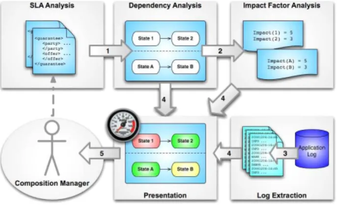
Fig. 1 depicts the implementation of MoDe4SLA. At design time, we analyze relations between services and the composition with respect to the agreedresponse timeand costsof the different providers (Step 1 in Fig. 1). The result of this dependency analysis constitutes the input for a subsequent impact analysis (Step 2). During runtime, event logs are analyzed using the event log model, filter- ing events referring to services and their SLA statements (Step 3). These results, together with impact analysis and dependencies, constitute input for the monitoring interface (Step 4). The latter enables time efficient composition management and maintenance (Step 5).

To support the informal approach presented in [7], this paper introduces formalization of dependency analysis and feedback models. The formalization is supported by a proof-of-concept implementation. The latter provides a means to analyze randomly generated Web service compositions at design time, and to monitor its dependencies and impact during runtime. The innovation of this paper is a

(2)

Figure 1. MoDe4SLA Approach

method that processes monitoring data to analyze impact with regard to different (QoS) criteria (i.e., instance-based monitoring) rather than monitoring each service invocation independently.

In Section 2 we describe an informal summary of the contribution after which we give an overview of our approach in Section 3. Sections 4, 5, and 6 describe the formalization process. In Section 7 we present our proof-of- concept implementation. We conclude with related work and a summary in Sections 8 and 9.

2. Impact Factors

To determine which service(s) cause SLA violations of the composition, we determine the performance of each individual service and whether this influences the composition SLA, i.e., whether the service has an impact on the composition. Each SLA consists of several Service Level Objectives (SLOs). Common SLOs are agreements on response time, availability, and costs. Intuitively, if a service is invoked often and it has a high SLO value then it has a high impact on the composition. In [7] we give an intuitive description on how to combine the number of invocations and realized SLO value by multiplication.

However, this intuitive notion of impact is not sufficient to capture real-life complexity. Consider Fig. 2 representing a service composition where each run invokes two services in parallel: either S1 and S2, or S1 and S3. Intuitively, the expected impact for S1 is 1·10 = 10since it is invoked every invocation (i.e.,1) and responds in10ms. S2 has an impact of0.5·20 = 10and S3 of0.5·30 = 15, assuming both have50%chance of being chosen per invocation.

However, in practice structure (i.e., expected number of invocations) and performance (i.e., SLO value) do not suf- fice to describe the realized impact. It can be expected that most times, S1 finishes before the other service (faster response time). Therefore, S1 does not contribute to overall

response time since this is done by the longer running service. In fact, the setting in which the services run (e.g., running parallel with high response time services) should be taken into account as well.

Figure 2. Service Composition Example

We calculate the impact factor (IF) of each service in the composition asabsolute valueindicating the serviceimpact shareof the composition for a specific SLO (e.g. response time). By definition, the IFs of the different services add up to1.0, and are now determined bystructure of the compo- sition(e.g., parallel running services and estimated number of invocations),performance of the particular service(e.g., expected response time), andperformance of other services in the composition.

3. Overall Approach

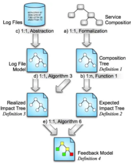
To automatically derive dependency relations from the composition structure and the SLAs, we propose tree-based formal transformations as depicted in Fig. 3. The composition structure is represented as the composition tree(cf.

Fig. 3 a). The structure could be derived, for example, from a BPEL process model. Since composition performance is dependent on the performance of the services, we analyze per SLO the expected impact of each service. By combining the structure and the agreed upon level of service, we calculate for each considered SLO at design time theexpected impact tree (cf. Fig. 3 b). Since agreements are often vi- olated, we monitor at runtime the realizedimpact on the composition for each service. Necessary monitoring information is abstracted from log files (cf. c). Together with the composition this monitoring information is used to calculate therealized impact tree(cf. d). Thefeedback modelis a performance indicator of the service composition since it shows the difference between expected and realized values (cf. e).

4. Design Time

At design time we analyze dependencies of the composition on its underlying services. We determine the expected impact of each service on the overall composition for a specific SLO. A service composition is modelled as a

(3)

Figure 3. Structural Approach

tree where the top vertex represents the service composition (COMP) and the leafs represent Web services (WS). Con- necting vertices and edges depict composition structure. Es- timations on the number of invocations are captured by annotating vertices and edges with estimated or agreed upon values. For example, two edges leaving an XOR vertex are annotated with the probability an edge will be chosen. We consider the most commonly used workflow patterns [1] as constructs. Details on vertices are explained in the following.Composition treesare defined as follows:

Definition 1 (Composition Tree) Let Vs be the set of types for service vertices {W S, COM P} and let Vc

be the set of structural vertices: {AN D, AN DDISC, OR, XOR,ORDISC, LOOP, SEQ}. A composition tree is a 6-tupleCT(V_c,V_s) = (V, E, ρ, µ, τ, σ), with

• V is a set of vertices,

• E:V →V is a set of directed edges,

• ρ:E→Rthe probability of selection compared to its siblings,

• τ:V → Vc∪ Vsspecifies the vertex type,

• σ:{v∈V |τ(v)∈ Vs} 7→Rⁿspecifies the expected SLO values for each SLO, wherenindicates the num- ber of SLOs,¹

• µ:{v ∈V |τ(v)∈ Vc} 7→(ε∪R)³annotations of structural vertices are 1) number of started services, 2) number of discriminative success, and 3) number of iterations.

Based on the composition, expected runtime behavior is calculated resulting in an expected impact tree. Such a

1We assume that all vertices are annotated with the same tuple of SLOs.

Composition Response Time Cost

AND max(total) sum(total)

AND DISC max(subset) sum(subset)

OR max(subset) sum(subset)

OR DISC max(subset) sum(subset)

XOR max(one) sum(one)

Loop sum(total^∗) sum(total^∗) Sequence sum(total) sum(total)

Table 1. Vertex Matching between Trees tree depicts for an SLO the expected impact of a service per composition invocation. This supports identification of services with high influence on composition behavior. The type of considered SLO determines the transformation algorithm. For example, revisit the example in Fig. 2. Each invoked service has an impact on the composition costs.

However, only the slowest responding service influences the composition response time. For each monitored SLO a tree is created (e.g., one for response time and one for costs).

Table 1 shows the types of relations between services per SLO (response time and cost) and construct. Although there exist more SLOs to consider (e.g., availability), this table suffices to demonstrate the principle of our approach.

A parallel AND split and AND join (cf. AND in Table 1) succeeds after the slowest responding service finishes (i.e., max(total)), and its total cost is the sum of all invoked services (i.e., sum(total)). For a parallel AND split with discriminative join (AND DISC), a parallel OR split with a discriminative join (OR DISC), and a parallel OR split with normal join, the response time is determined by the slowest invoked service (i.e., max(subset)) and the cost corresponds to the sum (i.e., sum(subset)). For sequences (Sequence) and for sequences executed more than once (Loop) both response time and cost are summed up for all invoked services (sum(total) and sum(total^∗), where∗indicates the number of iterations). For an XOR split and join the invoked service contributes to response time and cost (i.e., max(one) and sum(one)).expected impact treesare defined as follows:

Definition 2 (Expected Impact Tree) LetVs be the set of service vertices{W S, COM P}and letVibe the set of de- pendency vertices: {max(total), max(subset), max(one), sum(total), sum(subset), sum(one), sum(total^∗)}. An expected impact tree is a 5-tuple EIT(Vi,Vs) = (V, E, ρ, τ, σ), where

• ρ:E→Rthe probability of contribution per compo- sition invocation,

• τ :V → Vi∪ Vsspecifies the type of the vertex,

• σ : {v ∈ V | τ(v) = W S} 7→ R×R Annota- tions of Web service vertices are in the first dimension

(4)

“estimated impact”, and in the second dimension “ex- pected SLO value”,

• σ : {v ∈ V | τ(v) = COM P} 7→ R annotation of composed services specifies estimated SLO value based on composition structure.

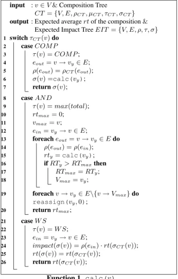
We only introduce algorithms for response time. Due to lack of space, only parts of the algorithm are provided formally (pseudo code), the remaining parts are described verbally. The goal of the expected impact tree is threefold:

input :v∈V&Composition Tree

CT ={V, E, ρCT, µCT, τCT, σCT} output: Expected averagertof the composition&

Expected Impact TreeEIT ={V, E, ρ, τ, σ}

switchτCT(v)do

1

caseCOM P

2

τ(v) =COM P;

3

eout=v→vy∈E;

4

ρ(eout) =ρCT(eout);

5

σ(v) =calc(vy);

6

returnσ(v);

7

caseAN D

8

τ(v) =max(total);

9

rtmax= 0;

10

vmax=v;

11

ein=vy→v∈E;

12

foreacheout=v→vy∈Edo

13

ρ(eout) =ρ(ein);

14

rty=calc(vy);

15

ifRTy> RTmaxthen

16

RTmax=RTy;

17

Vmax=vy;

18

foreachv→vy∈E\{v→Vmax}do

19

reassign(vy,0);

returnrtmax;

20

caseW S

21

τ(v) =W S;

22

ein=vy→v∈E;

23

impact(σ(v)) =ρ(ein)·rt(σCT(v));

24

rt(σ(v)) =rt(σCT(v));

25

returnrt(σCT(v));

26

Function 1 calc(v)

• Estimate the behavior of the overall composition based on both the contracts (SLAs) with the different service providers and the structure of the composition (i.e., calculate theσ-value).

• Estimate the impact (e.g., on response time) of each subtree on the overall composition (i.e., calculate the ρ-value for the edges).

• Estimate the impact (e.g., on response time) of each Web service on the overall composition (i.e., calculate theσ-value for the Web service).

All these estimations are based on contracts with the service providers and on the structure of the composition. Both expected QoS and structure determine estimated probability that a service isinvoked. As described, invocation of a service does not necessarily mean it actuallycontributes to, for example, the response time (e.g., in parallel running branches only the longest running has an impact). There- fore, Func. calc(v) determines the probability a service gets invoked and it actually contributes to the overall composition.

input:v∈V andz=ρof incoming edgev ein=vy→v∈E;

1

ρ(ein) =z;

2

switchτCT(v)do

3

caseXOR

4

foreacheout=v→vy∈Edo

5

reassign(vy, ρ(ein)·ρCT(eout));

caseAN D

6

foreachv→vy∈Edoreassign(vy, ρ(ein));

7

Function 2 reassign(v, z)

VerticesV and edgesEof the expected impact tree are equal to vertices V and edgesE of the composition tree.

Thestructureof both trees is equal, thoughannotationand namingof vertices and edges differ. The function traverses recursively through the composition tree, starting with the composition (COM P) vertex. Its calculations can be di- vided in five steps.

Firstly, when traversing the tree thename of each vertex (τ-value) is determined by its original type (cf. calc(v) in line 3, 9, & 22). For example, a parallel split is named max(total) in the expected impact tree for response time (cf.

Table 1). Secondly, theprobability each edge gets invoked (cf. calc(vy), ρ assignment line 5 & 14) is determined by combining its local probability with the probability its parent edge gets invoked. Now, each Web service “knows”

locallyits probability to be invoked per composition invocation. Thirdly, each vertex determines itsexpected average response time based on the expected response times of its children (i.e., the expected response times of services invoked in that subtree). For example, incalc(v) lines 13- 15 an AND vertex determines its expected response time based on the maximum response time of all its children.

Fourthly, each vertex determines which children branches will have an impact if they are chosen (i.e.,expected con- tribution). For example, if an AND vertex has one fast responding child compared to the other children then this child will most likely not contribute to the composition re-

(5)

sponse time since it finishes before the rest (cf. calc(v), lines 16-18). Now, each vertex hasglobal knowledge on expected behavior of its children. Fifthly, this global information is propagated through the tree, annotating each branch with the probability it contributesto the composition per invocation (cf. Func. reassign(vy, n) invoked bycalc(v) in line 19).

The calculation code is not shown for OR split with discriminative join because the code is longer and the general principal has been shown for the AND case (line 8). Infor- mally, for each subsetsof branches from the OR split we calculate likelihood l of invocation and its response time.

Since it is a discriminative join, the expected response time depends on the fastest responding subsets⁰. For example, if four out of five branches are started, and three need to finish for the discriminative join to succeed, the theoretical min- imum response time can only be the response time of the third-quickest service. Comparable calculations are done for the remaining vertex types.

5. Runtime

At runtime we gather monitoring data from log files in alog file model. To determine composition performance, we analyze each composition invocation the impact of each service on, for example, response time. Results are represented in therealized impact treewhere average impact of each service on the composition is depicted.

Log file modelMis an abstraction of log files containing data on composition invocations. Each invocation is represented as a list of invoked Web services for that composition instance. Each element in the list is a 4-tuple containing a time stamp (ts), the name of the invoked Web service (ws), its costs (costs), and its response time (rt). It needs to be determined which tuples (i.e., service invocations) in the log file model belong to a specific service composition invocation. We accomplish this correlation by analyzing different time stamps on the service invocations in combination with the service composition structure. A detailed description of this correlation of events is out the scope of this paper (see [6]). The realized impact tree is defined as follows:

Definition 3 (Realized Impact Tree) Let Vs be the set of service vertices {W S, COM P} and let Vi be the set of dependency vertices{max(total), max(subset), max(one), sum(total), sum(subset), sum(one), sum(total^∗)}. A re- alized impact tree is a 5-tuple RIT = (Vi,Vs) = (V, E, ρ, τ, σ), where

• ρ:E →Rthe average contribution per composition invocation,

• τ:V → Vi∪ Vsspecifies the vertex type,

• σ : {v ∈ V | τ(v) = W S} 7→ R×Rannotations of Web service vertices are in the first dimension: total contributed SLO value, and in the second dimension:

total number of contributions,

• σ:{v∈V |τ(v) =COM P} 7→R×Rannotations of the composition node is in the first dimension: total realized SLO value, and in the second dimension: total number of invocations.

The goal of the realized impact tree is threefold:

• Determine realized behavior of the service composition over a specific period of time (i.e., calculateσ),

• Determine realized impact each subtree has on the overall composition (i.e.,ρ-value of the edges), and

• Determine realized impact of each Web service on the composition (i.e.,σof the Web service vertices).

VerticesV and edgesE of the realized impact tree are equal to the vertices and edges in the composition. Alg. 3 shows implementation for response time. The code is only shown for a subset of vertex types due to lack of space. As argued before, not every Web service invocation eventually contributes to the SLO value of the composition. There- fore, Alg. 3analyzes all entriesin the log file model (line 3, Alg. 3) and determines, based on composition structure and other services performance, which entries (i.e., which Web service invocations) impact the composition. For this, recursive Func. addWS(v) is invoked in line 5 of Alg. 3.

For example, the XOR split determines which children (cf.

line 20 of Func. addWS(v)) contribute to the overall response time (cf. line 22-26) and returns all contributing Web service invocations in the subtree (cf. conf irm, line 27). These entries are added to theconf irmedlist (line 6, Alg. 3). Secondly, all confirmed entries are used toupdate total response time and total number of invocations (i.e.,σ- values) of the services (lines 7-10, Alg. 3).

As a last step, Alg. 3 determines contribution per composition invocation (i.e.,ρ-value) for each edge by invok- ing recursive Func. calcImpact(vcomp) in line 11. This function determines the number of contributions per composition invocation for each edge (i.e., its ρ-value). Web service leafs calculate ρ-value of the incoming edge (cf.

line 16-19 of Func. calcImpact) by comparing number of leaf node invocations with total number of composition invocations. For example, if the composition is invoked 6 times and the leaf node contributes 3 times then it contributes on average0.5times to each composition invocation. Each structural node combines information of its outgoing edges and determines theρ-value of the incoming edge. For example, in an AND split the overall contribution of the subtree is the summation ofρ-values of its outgoing edges (cf. lines 11-14).

(6)

input : Log File ModelLand Composition Tree CT = (V, E, ρCT, µCT, τCT, σCT) output: Realized Impact TreeEIT = (V, E, ρ, τ, σ) conf irmed=∅;

1

vcomp={v|τCT(v) =COM P};

2

foreachl∈Ldo

3

initially=l;

4

(cf, rt, ts) =addWS(vcomp);

5

conf irmed=conf irmed∪cf;

6

foreachtuple∈conf irmeddo

7

v=ws(tuple);

8

rt(σ(v)) =rt(σ(v)) +rt(tuple);

9

contribution(σ(v)) + +;

10

ρ=calcImpact(vcomp);

11

Algorithm 3: realized impact

6. Feedback Model

The feedback model depicts deviations from agreed upon SLA values by comparing estimated and realized impact trees. Colors on edges and vertices are used to visualize these deviations. Currently, red, green, yellow, darkgreen, and colorless are used (i.e.,θ-values) but these can be ex- tended or changed in any preferred way. Intuitively, red and yellow represent negative deviations while green and darkgreen represent positive deviations.

Definition 4 (Feedback Model) LetC be the set of colors {red, green, yellow, darkgreen, no color}. A feedback model is a 6-tupleFM(Vi,Vs,(C)) = (V, E, ρ, τ, σ, θ), where

• ρ :E →Rrealized average contribution per composition invocation,

• τ :V → Vi∪ Vsspecifies vertex type,

• σ:{v∈V |τ(v) =W S} 7→Rspecifies realized impact,

• θ : E → C specifies the deviation between realized and estimated contribution,

• θ : {v ∈ V |τ(v) = W S} 7→ C specifies the deviation between average contributed value and agreed upon SLO value,

• θ:{v∈V |τ(v) =COM P} 7→ Cspecifies the deviation between realized average value and agreed upon SLO value.

The goal of the feedback model is to support management in identifying causes for badly performing compositions. We accomplish this by giving feedback on:

1. Deviation between expected and realized behavior of the composition regarding an SLO (i.e., itsθ-value), 2. Deviation between expected and realized contribution

of each subtree to the composition,

3. Deviation between expected and realized contribution of each Web service in the composition, and

input :v∈V

output:(conf irm, rt, ts): the set of contributing tuples conf irm, with its overallrt, and thetsof the first started tuple∈conf irm

conf irm=∅;

1

rt= 0;

2

ts=M ax;

3

switchτCT(v)do

4

caseCOM P

5

v→vchild∈E;

6

(conf irm⁰, rt⁰, ts⁰) =addWS(vchild);

7

rt(σ(v)) =rt(σ(v)) +rt⁰;

8

invoc(σ(v)) + +;

9

return(conf irm⁰, rt⁰, ts⁰);

10

caseAN D

11

foreachv→vchild∈Edo

12

(conf irm⁰, rt⁰, ts⁰) =addWS(vy);

13

ifrt⁰> rtthen

14

rt=rt⁰;

15

conf irm=conf irm⁰;

16

ts=ts⁰;

17

return(conf irm, rt, ts);

18

caseXOR

19

20

(conf irm⁰, rt⁰, ts⁰) =addWS(vy);

21

ifconf irm⁰6=∅ ∧ts⁰< tsthen

22

ifconf irm6=∅then

23

initially=initially∪conf irm;

rt=rt⁰;

24

conf irm=conf irm⁰;

25

ts=ts⁰;

26

27

caseW S

28

foreachtuple∈initially, ws(tuple) =vdo

29

ifts(tuple)< tsthen

30

rt=rt(tuple);

31

conf irm=tuple;

32

ts=ts(tuple);

33

ifconf irm6=∅then

34

initially=initially\conf irm;

35

36

else

37

return(∅,0,0);

38

Function 4 addWS(v)

(7)

input :v∈V

vcomp=vx∈V, τCT(vx) =COM P;

1

ein=vy→v∈E;

2

switchτCT(v)do

3

caseCOM P

4

τ(v) =COM P;

5

ρ=calcImpact(vchild);

6

returnρ;

7

caseAN D

8

τ(v) =XOR;

9

contribution= 0;

10

11

ρchild=calcImpact(vchild);

12

contribution=contribution+ρchild;

13

ρ(ein) =contribution;

14

returnρ(ein);

15

caseW S

16

τ(v) =W S;

17

ρ(ein) =contribution(σ(v)) invoc(σ(v_comp)) ;

18

returnρ(ein);

19

Function 5 calcImpact(v)

4. Realized contribution per invocation of Web services (i.e.,σ-value) and subtrees (i.e.,ρ-value).

VerticesV and edgesEof feedback model are equal to vertices V and edges E of estimated and realized impact tree. Alg. 6 calculates the feedback model by computing for each Web service vertex what its composition impact is, e.g. line 5, Alg. 6. This depends on number of contributions per composition invocation (i.e.,ρ-value) and average SLO when invoked (i.e.,σ-value). Assume Web service S1 has an average response of 10 ms, against 20 ms of the composition. If S1 contributes in fifty percent of the composition invocations (i.e.,ρ= 0.50) then the impact factor of S1 is

10

20 ·0.50 = 0.25. On average S1 determines25% of the composition response time.

Furthermore, the color of each Web service and composition is determined by invokingcolor(real, est) in line 6 and 7 of Alg. 6. This function determines deviation between realized and estimated values as depicted in Func. 7.

Each edge is annotated with the realized contribution per composition invocation in line 9 and colorθis determined by deviation between expected and realized contribution in line 10.

7. Implementation

7.1. Generation and Execution

The generation of test compositions is performed with an extended version of the SENECA simulation environ-

input :EIT(V, E, ρE, τE, σE)and RIT(V, E, ρR, τR, σR) output:F M(V, E, ρ, τ, σ, θ) vcomp=v∈V, τE(v) =COM P;

1

foreachv∈V do

2

τ(v) =τR(v);

3

ifτ(v) =W Sthen

4

σ(v) = _rt(σ^rt(σ^R^(v))

R(vcomp))·ρR(ein);

5

θ(v) =color(σ(v), impact(σE(v)));

6

ifτ(v) =COM Pthenθ(v) =

7

color(_invoc(σ^rt(σ^R^(v))

R(v)), impact(σE(v)));

foreache∈Edo

8

ρ(e) =ρR(e);

9

θ(e) =color(ρ(e), ρE(e));

10

Algorithm 6: feedback model

input :real: realized value,est: estimated value output:color: the color of the edge or vertex deviation=^real−est_est ·100;

1

ifdeviation≥10then returnred;

2

if10> deviation≥5then returnyellow;

3

if5> deviation≥ −5then returngreen;

4

ifdeviation <−5then returndarkgreen;

5

Function 7 color(real, est)

ment [10]. This simulation environment implements a) a structural model of service compositions and b) a QoS model for the handling of QoS attributes of the services in the composition. The generation of compositions is performed randomly with particular input parameters. The parameters are the number of services in total and the range of the planned QoS delivered. Then the software generates - by using the standard random number generator of the Java platform - the following two main parts.

Firstly, thestructure of the composition. At a given point, the generation software decides between placing a service or a composition structure containing services, both with equal probability. By this scheme, compositions can result in a flat sequence of services or contain nested structures forming a more sophisticated execution plan. There are seven basic executions patterns [10] chosen from the workflow patterns by Aalst et al. [1].

Secondly, theactual QoS delivered by the service. At the beginning, this function was used to perform the optimisa- tion simulations for optimising the QoS of service compositions [10]. The generation software has set particular QoS attributes for different candidates in order to select the op- timal set of services for the composition according to their QoS. For MoDe4SLA, it is assumed that the selection has taken place and accordingly only one (chosen) service with a particular QoS is required. But in addition, the genera-

(8)

tor will randomly generate a probability that is taken at run time to decide whether a service should fail or not. By these two elements, the generator builds up a data structure in application memory that allows the environment to simulate the execution of a service composition.

The simulation performs on the generated test service composition with its QoS attributes as described in the section above. The discrete event simulation simulates the pass of a second (this is the unit of the simulated response time SLO), and tracks the progress among the services of the composition. If a service is finished, then the next service is triggered according to the execution plan. Each service implements the simulation to either start or finish the work as planned. In addition, a random function allows to cancel the execution or miss the planned QoS by running for a longer time. The probability that a particular service fails or runs longer is set at generation time. By this scheme, randomly failing services are simulated. The simulation software generates a log output that tracks a failure of the service. This log is used to perform the impact analysis.

7.2. Feedback Models

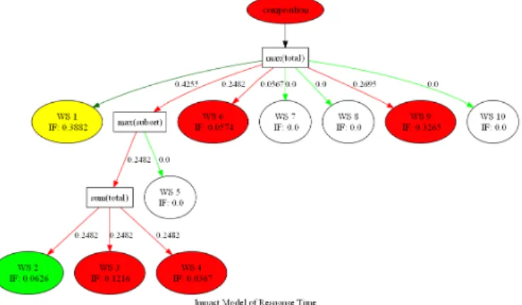
Service developers receive information on the composition performance through the graphical feedback model as generated by the simulator (cf. Fig. 4). The information can be used to evolute the composition by tuning the structure or renegotiate SLAs of the services. A red colored service indicates worse performance than agreed upon in the SLA, while green indicates proper performance of the service. Yellow indicates the service is not performing perfectly but still within the boundaries set by the company, and dark green indicates a service running even better than the company anticipated. Uncolored services indicate that these never contributed to the overall response time in the considered log file. Therefore, their impact is zero. The edges are colored in the same manner, for example, red indicates the edge contributes more often than expected. Fig. 4 indicates that the SLO for response time of the composition is not met (i.e., it is colored red). Bad performance in this case is caused by two factors. Firstly,Performance of the services: together, services 1, 3, and 9 have an im- pact factor (IF) of over80%and each service responds on average slower than agreed upon (i.e., yellow or red). Sec- ondly,Structure of the composition: badly performing ser- vices 3 and 9 are contributing more often than expected (i.e., red incoming edges). The impact and contribution factors in combination with the coloring eases the identification of bad performing services with a high impact so that management of compositions with many services becomes more straightforward.

In this case, we can derive that either badly performing services should be replaced or renegotiated (e.g., service 1,

3, and 9), the SLA agreement with the customer has to be tuned down (i.e., offer less performance), or the structure of the composition has to be adapted so that it suits real-life behavior. Furthermore, we can conclude that services 5, 7, 8, and 10 have no impact on the composition and therefore do not need to be considered for a causal analysis of bad performance, saving valuable analysis time.

Figure 4. Feedback Model

8. Related Work

The work of Casati et al. [13] aims at automated SLA monitoring by specifying SLAs and not only considering provider side guarantees but focus also on distributed monitoring, taking the client side into account. Pistore et al. [3]

enable run-time monitoring while separating business logic from monitoring functionality. For each instance a monitor is created. Contribution of this approach is the ability to also monitor classes of instances, enabling aggregation of impact of several working instances. Smart monitoring [4] implements the monitor functionality itself as service. Three types of monitors handle different aspects of the system.

Their approach is developed to monitor contracts with con- straints. Further work of Baresi et al. [5] presents an approach to dynamically monitor BPEL processes by adding monitoring rules to them. In contrast, our approach does not require modifications to the process descriptions and thus requires less effort to apply to some application areas.

An interesting approach in this direction is work by [11]

which, as an exception, does consider the whole state of the system. They aim at monitoring behavioral system deriva- tions. Monitoring requirements are specified in event cal- culus and evaluated with run-time data. Although many of above mentioned approaches consider services provided by third parties and allow abstraction of results for composite services, none of them addresses how to create this abstrac-

(9)

tion in detail. E.g., matching messages from different processes where databases are used are not considered.

Menasce [12] presents response time analysis of composed services to identify impact of slowed down services.

The impact on the composition is computed using a Markov chain model. The result is a measure for the overall slow down depending on statistical likelihood of a service not delivering expected response time. As opposed to our approach, Menasce performs at design-time rather than providing an analysis based on analyzing runtime data. In addition, our work provides a framework to cover structures beyond a fork-join arrangement.

A different approach with the same goal is virtual resource manager proposed by Burchard et al. [8]. This approach targets a grid environment where a calculation task is distributed among different grid nodes for individual computation jobs. If a grid node fails to deliver the promised service level, a domain controller first reschedules the job onto a different node within the same domain. If this action fails, the domain controller attempts to query other domain controllers for passing over the computation job. Although the approach covers runtime, it follows a hierarchical auto- nomic recovery mechanism. MoDe4SLA focusses on identifying causes for correction on the level of business opera- tions rather than on autonomous job scheduling. Further, in critical path analysis (CPA) for resource management the preferred order of tasks is determined by analyzing the graph containing all possible paths [14]. However, in CPA each path shows one possible execution while in our analysis the complete graph depicts one execution. Furthermore, in MoDe4SLA we compare estimated with realized behavior which is not done in CPA.

Another research community analyzesroot causesin services. Dependency models are used to identify causes of violations withina company. For example, [2] determine the root cause by using an approach based on dependency graphs. Especially finding the cause of a problem when a service has an SLA with different metrics is a challenging topic. Also [9] uses dependency models for managing internet services, again, with focuss on finding internal causes for problems. MoDe4SLA identifies causes of violations in other services rather than internally. Furthermore, our dependencies between different services are on the same level of abstraction while in root cause analysis one service is evaluated on different levels of abstraction.

9. Summary and Outlook

In this paper we describe a formal approach to support management of composite services by analyzing impact factors on service compositions. In continuation of previ- ous work we have now shown the details and feasibility of our approach. The algorithms in pseudo code serve as

a blueprint for our proof-of-concept implementation which supports simulation of service composition runs and the analysis of runtime results. In near future we plan to ex- tend our approach by providing interpretation guidelines for the feedback models to enhance decision making on service composition management. We will use the impact factors to provide reconfiguration suggestions.

References

[1] Workflow patterns. http://www.workflowpatterns.com.

[2] M. K. Agarwal, K. Appleby, M. Gupta, G. Kar, A. Neogi, and A. Sailer. Problem determination using dependency graphs and run-time behavior models. InDSOM, volume 3278, pages 171–182. Springer, 2004.

[3] F. Barbon, P. Traverso, M. Pistore, and M. Trainotti. Run- time monitoring of instances and classes of web service compositions. InICWS ’06, pages 63–71, 2006.

[4] L. Baresi, C. Ghezzi, and S. Guinea. Smart monitors for composed services. InICSOC ’04, pages 193–202, New York, NY, USA, 2004.

[5] L. Baresi and S. Guinea. Towards dynamic monitoring of WS-BPEL processes. InICSOC, volume 3826, pages 269–

282. Springer-Verlag, 2005.

[6] L. Bodenstaff, A. Wombacher, and M. Reichert. On formal consistency between value and coordination models. Tech- nical Report TR-CTIT-07-91, Univ. of Twente.

[7] L. Bodenstaff, A. Wombacher, M. Reichert, and M. C.

Jaeger. Monitoring dependencies for SLAs: The MoDe4SLA approach. InSCC 2008, pages 21–29, 2008.

[8] L.-O. Burchard, M. Hovestadt, O. Kao, A. Keller, and B. Linnert. The virtual resource manager: an architecture for SLA-aware resource management. Cluster Computing and the Grid, IEEE Int. Symposium on, 0:126–133, 2004.

[9] D. Caswell and S. Ramanathan. Using service models for management of internet services.IEEE Journal on Selected Areas in Communications, 18(5):686–701, 2000.

[10] M. C. Jaeger and G. Rojec-Goldmann. Seneca - simulation of algorithms for the selection of web services for compositions. InTES, pages 84–97, 2005.

[11] K. Mahbub and G. Spanoudakis. Run-time monitoring of requirements for systems composed of web-services: Initial implementation and evaluation experience. InICWS, pages 257–265, 2005.

[12] D. A. Menasc´e. Response-time analysis of composite web services.IEEE Internet Computing, 8(1):90–92, 2004.

[13] A. Sahai, V. Machiraju, M. Sayal, A. P. A. van Moorsel, and F. Casati. Automated SLA monitoring for web services. In DSOM ’02, pages 28–41, 2002.

[14] R. Willis. Critical path-analysis and resource constrained project scheduling-theory and practice. European Journal of Operational Research, 21(2):149–155, 1985.

[15] L. Zeng, B. Benatallah, A. H. Ngu, M. Dumas, J. Kalagnanam, and H. Chang. Qos-aware middleware for web services composition. IEEE Trans. Softw. Eng., 30(5):311–327, 2004.