Design of Normal-Conducting Rebuncher Cavities for the

(1)

Institute of Applied Physics IAP University of Frankfurt, Germany

Design of Normal-Conducting Rebuncher Cavities for the

MYRRHA Injector Linac

Master’s Thesis

submitted by Daniel Koser

Thesis Supervisors:

Prof. Dr. Holger Podlech Prof. Dr. Alwin Schempp

June 2015

(2)

(3)

Abstract

The MYRRHA project (Multi-purpose hYbrid Research Reactor for High-tech Applications) at SCK·CEN in Mol, Belgium, is currently being designed as an Accelerator Driven System (ADS) for high-flux neutron irradiation applications such as the demonstration of the technical feasibility of transmuting long-lived high-level radioactive waste on industrial scale. For operating the subcritical reactor core the dedicated driver linac is supposed to provide a continuous wave proton beam of 600 MeV and 4 mA in order to produce fast neutrons at the liquid lead-bismuth reactor coolant that serves as spallation target. Since frequently repeated beam interruptions would lead to high mechanical stress and fatigue on the reactor components it is crucial to ensure permanent beam availability, making reliability a key issue for the proton driver development.

The planned 600 MeV main linac consisting of superconducting spoke and elliptical cavities is intended to be supplied by a 17 MeV double injector linac that is developed at the Institute of Applied Physics (IAP) of the Goethe University Frankfurt and contains a 4-Rod-RFQ as well as a section of normal-conducting and superconducting CH-cavities. For longitudinal beam focusing the recent injector layouts additionally include a 2-gap and a 5-gap rebuncher structure with effective voltages of 80−116 kV and 290 kV, respectively, both operating at 176,1 MHz.

The 2-gap structure was developed from scratch and is going to be implemented as a coaxial quarter-wave resonator providing maximum shunt impedance and having convenient geometric dimensions. The overall RF-design including the tuning system, consisting of two small plunger tuner elements acting capacitively on the drift tube, as well as an inductive power coupling loop was optimized using CST Microwave Studio. Beam dynamics simulations investigating the effect of the electric dipole component caused by the open-ended stem were done using a new Particle- in-Cell code named BENDER which was developed at IAP. Thermal simulations concerning the layout of the water cooling system and structural mechanics simulations regarding the expansion of the thermally loaded stem were done with CST MPhysics Studio. Also the occurrence of multipacting was investigated by doing particle tracking simulations using CST Particle Studio.

The basic design of the 5-gap structure was to the greatest possible extend carried over from the CH-rebuncher prototype that was already designed and manufactured within the scope of the FRAnkfurt Neutron Source at the Stern-Gerlach-Zentrum (FRANZ). Adapting the gap geometry to the designated particle energy, increasing the aperture radius and applying a modified geometry for the cavity caps finally yielded a 5-gap CH-rebuncher that is perfectly suitable for the requirements of the MYRRHA injector linac.

(4)

[1] Introduction

Worldwide 437 nuclear reactors were in operation in the beginning of 2015, capable of generating a total electric power of 378 GW [51]. During 2014 nuclear electricity provided 2,4 PWh of electric energy corresponding to 11 % of the global electric energy generation.

The products of the nuclear fission contain besides short-lived isotopes with half-lifes ranging from a couple of hours to some years also very long-lived radionuclides like, among others,

99Tc (t_1/2 = 2,1·10⁵years) or ¹²⁹I (t_1/2 = 1,59·10⁷years) [48]. Moreover long-lived radioactive transuranic actinides like various isotopes of Np, Pu, Am and Cm with half-lifes of up to several 10⁶ years are produced by transmutation-decay chains beginning with ²³⁸U.

Typically a 1000 MWenuclear reactor produces about 25 tonnes of radioactive waste per year [51].

The contained amount of high-level radioactive waste (HLW) of roughly 3 % (≈750 kg) causes around 95 % of the overall radioactivity and would have to be isolated from the biosphere in deep geological repositories for millions of years due to the continuing tremendous radiotoxicity of its long-lived constituents. A contribution to a solution for this problem could be provided by the concept of Partitioning & Transmutation (P & T) [1] which intends to seperate the long-lived radiotoxic components out of the spent fuel (partitioning) and subsequently transmute them into radionuclides with substantially reduced half-lifes using an Accelerator Driven System (ADS) as described in the following. After all P & T could be capable of reducing the amount of transuranic elements by more than two orders of magnitude and decreasing the needed retention period to a few hundred years.

1.1 Accelerator Driven Systems

An Accelerator Driven System (ADS) is a subcritical nuclear reactor (k < 1) that serves as a multiplier for externally fed neutrons produced in a spallation target due to an impinging high energy proton beam. In order to generate the overall thermal reactor powerP_reactor,th an amount P_external = (1−k) ·P_reactor,th must be continuously provided from fission events induced by spallation neutrons (see Eq. 1.1).

P_external= I_beam e

N_n(E_p) Np

p_f,n E_f,n = (1−k)·P_reactor,th (1.1) With a given probability pf,n for neutron induced fission and Ef,n being the thereby released energy, P_external depends on the number of incident protons per time I_beam/e as well as on the energy dependent neutron yield per protonN_n(E_p)/N_p at the spallation target. Accordingly the overall thermal reactor powerPreactor,th =Pexternal·(1−k)⁻¹ can be adjusted with either the beam

(8)

[1] Introduction 1.2 MYRRHA & MAX

current Ibeam or the proton energy Ep. Fig. 1.1 shows a curve of experimentally obtained values of the neutron yield for different proton energies at a thick lead-bismuth target. The dependence of N_n/N_p on E_p decreases for higher energies and ranges fromN_n/N_p∝E_p³ atE_p ≈20 MeV to Nn/Np ∝Ep^0,7 atEp≈5 GeV [24].

Figure 1.1: compilation of measured values for the neutron yield per protonNn(Ep)/Np for different incident energiesE_pat a thick lead-bismuth target [24]

Figure 1.2:surface temperature variation at the inner reactor cladding for different durations of the beam interruption [2]

In case of beam interruptions the lacking neutron production at the spallation target leads to a termination of the chain reaction in the reactor core and the temperature of the reactor cladding and the contained components drops exponentially as depicted in Fig. 1.2. For beam trips with a duration of several seconds the temperature variations cause severe thermomechanical stress and the long-term fatique in case of frequent repetition would lead to short maintenance intervals and a limited overall operating time. The resulting requirement for permanent beam availability makes the reliability of the driver linac a key feature of the ADS configuration.

1.2 MYRRHA & MAX

The MYRRHA project (Multi-purpose hYbrid Research Reactor for High-tech Applications) at the Belgian nuclear research centre SCK·CEN located in Mol is conceived as an ADS type flexible fast spectrum research reactor operable in both critical and subcritical modes with the primary objective of demonstrating the technical feasibility of transmuting long-lived high-level radioactive waste on industrial scale [10]. Within this scope MYRRHA aims to provide a versatile multi-purpose neutron irradiation facility for fundamental research on general reactor physics and associated material sciences as well as for specific technical applications such as the production of radioisotopes for nuclear medicine or neutron irradiation of silicon for the fabrication of semi- conductors for power electronics. In addition a small fraction of the proton beam (<200µA) is used for the production of radioactive ion beams at the ISOL@MYRRHA experiment [11] that takes advantage of the unique permanent beam availability for high statistics measurements.

(9)

1.2 MYRRHA & MAX [1] Introduction

source

& LEBT RFQ _section^{rt CH} _section^{sc CH}

MYRRHA reactor source

& LEBT RFQ section^{rt CH} sc CH section

beam dump beam

splitter

< 4 mA , cw

17 MeV 80,8 MeV 184,2 MeV 600 MeV

< 200 μA, cw

ISOL@

MYRRHA β = 0,375 β = 0,51 β = 0,705

48x sc 2-gap spoke cavities 24 cryomodules 352,2 MHz

94x sc 5-cell elliptical cavities 32 cryomodules 704,4 MHz

double injector linac 176,1 MHz length ≈ 20 m

main linac tunnel length ≈ 240 m

Figure 1.3: conceptual scheme of the driver linac layout for MYRRHA¹ [21]

The MYRRHA reactor core is loaded with fast reactor MOX fuel (mixed plutonium-uranium oxide) and is cooled by a liquid lead-bismuth eutectic alloy (LBE) that provides suitable heat transfer properties but also serves as spallation target able to produce high neutron yields [24].

Based on safety considerations the criticality of the subcritical core for the ADS configuration with P_reactor,th ≈ 70 MW is intended to be around k = 0,95. The 600 MeV proton beam is delivered from the driver linac by a system of deflection magnets and injected into the reactor vertically from above as indicated in Fig. 1.3. At a beam current of up to 4 mA in Continuous Wave mode (P_beam = 2,4 MW) a neutron flux of about 2·10¹⁷n/s can be produced in the spallation target.

The ADS specific requirement of permanent beam availability is aimed to be satisfied within a margin of less than 10 beam trips longer than 3 s (defining a system failure) in an operational period of 3 months thus demanding a Mean Time Between Failures (MTBF) of>250 h. Further- more the number of allowed beam trips longer than 0,1 s is restricted to a value of 100 per day while beam trips of less than 0,1 s are tolerated without limitation.

The superconducting main linac consists of an intermediate energy part (17 to 80,8 MeV) of 2- gap spoke structures operated at 352,2 MHz and a high energy section (80,8 to 600 MeV) of 5-cell elliptical cavities at 704,4 MHz. A high fault tolerance is achieved by providing serial redundancy thus allowing to compensate the malfunction of a faulty cavity by increasing the gradients in the adjacent structures. The low energy section (30 keV to 17 MeV) operated at 176,1 MHz in conjunction with the proton source and LEBT acts as injector to the main linac and is designed as a parallel redundant double configuration with a second identical beamline. The second injector is permanently run in hot standby and can take over the injection in case of fault detection in the first injector. General design principles for the driver linac are high modularity and conservative operating ranges for the components far from their technological limits.

The advanced driver linac design was developed within the scope of the MAX project (MYRRHA Accelerator EXperiment R&D) as part of the 7th Framework Programme for Research and Technological Development of the European Union. The follow-on project MYRTE (MYRRHA Research andTransmutationEndeavour) as part of Horizon 2020 initiates the engineering design and prototyping phase.

(10)

[1] Introduction 1.3 The 17 MeV MYRRHA Injector Linac

1.3 The 17 MeV MYRRHA Injector Linac

The 4 mA proton beam is delivered with 30 keV by a Pantechnik Monogan M-1000 Electron Cy- clotron Resonance (ECR) ion source. The low energy beam transport and focusing is achieved by a pair of solenoid magnets with integrated dipole steerers and an RFQ interface section hosts an electrostatic chopper for creating a pulsed beam structure allowing to regulate the average beam intensity [45]. Out of the continuous proton beam injected from the LEBT the 4-Rod-RFQ [7]

generates transversally focused beam bunches accelerated to 1,5 MeV.

quadrupoleXdoubletX/Xtriplet steererXmagnet

bellow

beamXtransformer beamXpositionXmonitor

diagnosticXchamber collimator

phaseXprobe

22,2Xm

16,7Xm

19,5Xm MAXXalternativeXdesign

MAXXconsolidatedXalternativeXdesign

MAXXreferenceXdesignX2014

RB1 RB2

Figure 1.4: revised designs for the MYRRHA injector linac [36]

number W_s U_eff βλ/2 r_aperture `

of gaps [MeV] [kV] [mm] [mm] [mm]

MAX alternative design RB1 2 1,5 116 48,1 10 198,1

RB2 5 4,3 380 81,1 12,5 474,4

MAX consolidated alternative design

RB1 2 1,5 86 48,1 10 198,1

RB2 5 3,6 290 (270)² 74,3 10 (15)³ 447,3

MAX reference design 2014 RB1 2 1,5 80 48,1 15 198,1

RB2 2 1,5 90 48,1 15 198,1

Table 1.1:basic design paramaters (particle energyW_s, effective voltageU_eff, distance between gap centersβλ/2, aperture radiusrapertureand total length`) for the rebuncher cavities included in the MYRRHA injector designs

(11)

1.3 The 17 MeV MYRRHA Injector Linac [1] Introduction

Fig. 1.4 depicts the recently revised designs for the MYRRHA injector linac that were developed as an improvement over the MAX reference design 2012. In each design the RFQ is followed by a normal-conducting section since based on experience the provided particle distribution contains halo particles that get lost in the subsequent structures and would damage the sensitive surface of superconducting cavities thus increasing the probability of quenches. Also for low particle velocities the resulting compact cavity geometries cause problems concerning the RF-design of superconducting structures. The generally well-spaced intermediate cavity design and the conical geometry of the cavity caps provide enough room for beam diagnostics and focusing elements and allow a good accessibility and mountability of the components.

The normal-conducting section of the MAX alternative design and its consolidated version consists of a 2-gap rebuncher cavity followed by four constant-φ CH-cavities with 5 to 7 gaps and another 5-gap CH-rebuncher. Whereas in the superconducting section of the alternative design each of the eight constant-β 5-gap CH-cavities is hosted in its own cryomodule the shorter consolidated design comprises six 5-gap cavities that are contained pairwise in three cryomodules.

Both alternative designs provide a similar beam quality of the ejected 17 MeV proton beam with a reduced emittance growth compared to the MAX reference design 2012.

The MAX reference design 2014 pursues the concept of a smooth particle acceleration with rel- atively low field gradients in the first accelerating structures behind the RFQ and provides the best beam quality of the revised injector designs. The normal-conducting section consists of two

Figure 1.5:prototype of a 5-gap CH-rebuncher⁴ for FRANZ [47]

2-gap rebuncher cavities followed by an array of seven CH-structures in a 3−4−5−6−7−9−9 gap configuration with effective field gradients E_a = U_eff/` of up to 1,3 MV/m and a power dissipation <30 kW/m. The low divergence of the longitudinal phase spread at the exit of the CH-array makes a dedicated multigap rebuncher structure like in the previous injector designs obsolete. Housed in individual cryomodules the superconducting section contains five CH-cavities in a 3−5−6−6−6 gap configuration with effective field gradients of up to 4 MV/m.

Tab. 1.1 summarizes the design parameters for the rebuncher cavities of all three injector designs. Fig. 1.5 shows the copper-plated 5-gap CH-rebuncher prototype which was developed at IAP as part of the FRANZ beamline.

(12)

[1] Introduction 1.3 The 17 MeV MYRRHA Injector Linac

0 150 300 450 600 750 900 1050 1200 1350 1500 -0,03

-0,02 -0,01 0,00 0,01 0,02 0,03

-30 -20 -10 0 10 20 30 -0,02

-0,01 0,00 0,01 0,02

-30 -20 -10 0 10 20 30 0 100 200 300 400 500 600 700 800 900 1000 1100 1200 1300

Δϕ7[deg]Δϕ7[deg]

ΔW7/7WsΔW7/7Ws

z7[cm]

MAX7consolidated7alternative7design

MAX7reference7design72014

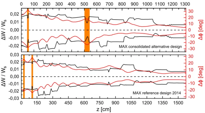
Figure 1.6: envelope (containing 99,73 % of the particles) of the longitudinal energy spread ∆W (black curve) and phase spread ∆φ(red curve) for the consolidated alternative design and the reference design 2014 of the MYRRHA injector linac (the rebuncher-sections are marked in orange) [36]

(13)

[2] RF Resonators & Linac Structures

In order to overcome the limitations of electrostatic accelerators, in which the total obtainable voltage is restricted to several MV due to electrical breakdown [16, p. 10], in 1924 Gustav Ising proposed a concept for particle acceleration based on the use of alternating electric fields, thus allowing to traverse the generated voltage multiple times [19]. Taking up on that a first prototype of an RF linear accelerator (linac) whose basic operating principle is similar to modern linacs was tested by Rolf Wideröe in 1927 [14, p. 1 f.]. A so called Wideröe linac consists of an array of drift tubes that are sequentially connected to opposite polarities of an RF source and are thereby periodically loaded against each other. As a consequence the phase of the electric field in adjacent acceleration gaps (space between the drift tubes) has a shift of 180^◦ (π-mode). In order to preserve the synchronicity between the transition of the accelerated particles (particle bunch) and the accelerating RF phase, the time between the transitions of adjacent gap centers (with a distance of `c) has to be equal to half the duration of the RF cycle. Hence`c has to be adapted gradually to the increasing particle velocity v = βc as well as to the RF frequency f = c/λ according to Wideröe’s condition `_c =βλ/2. It is apparent that for the acceleration of particles with highβ also high frequenciesf would have to be used in order to yield practicable values for

`cconcerning the overall length. Unfortunately at higher frequencies the drift tubes act as anten- nas and radiate a significant amount of energy into the electrically unenclosed surrounding space, leading to an impracticable low power efficiency. Inspired by the development of high-power RF amplifiers for radar systems operating at 200 MHz and higher, a solution was finally proposed by Luis Alvarez in 1946, who suggested enclosing the Wider¨oe linac with a conducting cylindrical structure in which the radiated energy is confined as an electromagnetic standing wave. The evolved Alvarez linac as explained further in section 2.3.2 is the precursor of the standing wave structures listed and described in the following sections that are standardly used as normal- or superconducting cavities in today’s hadron linacs.

2.1 Transmission-Line Resonators

In transmission-line resonators a standing electric current wave is excited on either a short- circuited or open-ended section of an RF transmission-line. Accordingly in the short-circuited case the length of the line segment is an integer multiple of half the wavelength (half-wave resonator), whereas in the open-ended case it is an odd multiple of a quarter of the wavelength (quarter-wave resonator). Although the shape of the enclosing structure has an influence on the resonance frequencyf0 = 1/(2π√

LC) by affecting the overall capacitance C and inductance L, the actual standing wave mode is solely determined by the geometry of the line segment, which is termed spoke or spiral in case of the accelerator structures discussed in the following sections.

(14)

[2] RF Resonators & Linac Structures 2.1 Transmission-Line Resonators

Another important linac structure that is a transmission-line resonator and not further mentioned is the 4-Rod-RFQ (radio-frequency quadrupole), in which a quarter-wave oscillation between the electrically open-ended adjacent electrodes (rods) is utilized [27, p. 21 ff.].

2.1.1 Coaxial Half-Wave Resonator

The simplified model of a coaxial half-wave resonator consists of an inner conductor (r = r₁) and a concentrically mounted outer conductor (r = r2) that are shorted out by conducting end walls at z = 0 and z = `. For this case it can analytically be shown that the boundary conditions at the inner and outer conductor (E_z =E_φ=B_r= 0 |_r=r₁_{, r=r}₂) and at the end walls (Er = Eφ = Bz = 0 |_{z=0, z=`}) allow transverse electromagnetic (TEM) resonant standing wave modes with no longitudinal field components (Ez =Bz = 0) [50, p. 22 ff.].

Figure 2.1: electric field distribution in a coaxial half-wave resonator

Figure 2.2: magnetic field distribution in a coaxial half-wave resonator The superposition of the current waves¹ I_z(t, z) =I₀eî(ωt−kz)andI−z(t, z) =I₀eî(ωt+kz) traveling on the inner conductor alongz and in the exact opposite direction, respectively, yields the total currentI_tot(t, z) =I_z(t, z)+I−z(t, z) = 2I₀cos(pπz/`)eîωt(withk=pπ/`,pbeing the mode number), allowing to calculate the azimuthal magnetic fieldB_φ(Eq. 2.1) in conjunction with Ampère’s law (H B dl~ =µ0

R~j dS). Given Faraday’s law (∇ ×E~ =−∂ ~B/∂t⇒∂Er/∂z =−∂B_φ/∂t) the radial electric fieldE_r (Eq. 2.2) can thus be obtained by integrating the time derivation ofB_φoverz (usingω=pπc/`,c= 1/√

µ₀₀ andi=e^iπ/2) from what subsequently follows thatE_φ=B_r = 0.

Accordingly the relationship between `and λis given by `=pλ/2.

B_φ(r, z, t) = µ₀I₀

πr cospπz

`

e^iωt (2.1)

Er(r, z, t) =− rµ0

0

I0

πrsin pπz

`

e^i(ωt+π/2) (2.2)

(15)

2.1 Transmission-Line Resonators [2] RF Resonators & Linac Structures

The stored energy W and the power loss Pc for the fundamental mode (p = 1, see Fig. 2.1 and Fig. 2.2) can be calculated from Eq. 2.32 and Eq. 2.33, using the maximum magnetic field level B_φ(r, z) =µ₀I₀cos(πz/`)/πr. Eq. 2.4 includes the losses on the inner and outer conductor and on both end walls.

W = µ0I02` 2π ln

r2

r₁

(2.3) P_c= RsI02

2π

4 ln r2

r₁

+ ` r₁ + `

r₂

(2.4)

2.1.2 Spoke Resonators

A half-wave cavity in which the transmission-line segment (that is also referred to as ‘spoke’) is mounted perpendicular to the axis of the cylindrical outer housing is generally termed as ‘spoke resonator’, whereas a so called ‘multi-spoke cavity’ is composed of several spokes (usually up to three), that are rotated by 90^◦ against each other. In multi-spoke structures each spoke on itself provides a half-wave mode as derived in the previous section [8, p. 15 ff.], but the overall superposition yields a field distribution that is fairly similar to the TE211 cavity mode like in CH-cavities (see section 2.3.3).

Accordingly the transverse dimension of spoke cavities is given by D_c = 2R_c =λ/2−x ≈λ/2 with x ≥0 depending on the total capacitive load. Commonly spoke resonators are used in the frequency range between 150 and 800 MHz and for velocities of 0,1 > β >0,5 [42, p. 13] and are due to their rigid mechanical structure and low magnetic surface fields often used as superconducting structures like depicted in Fig. 2.3, Fig. 2.4, Fig. 2.5 and Fig. 2.6.

Figure 2.3: superconducting coaxial half-wave resonator (f = 172 MHz, β = 0,27) for the RIA driver linac at Argonne National Laboratory [25]

Figure 2.4: superconducting single-spoke cavity (f = 325 MHz, β = 0,22) for the Project X linac at Fermilab [29]

Figure 2.5: superconducting double- spoke cavity (f = 345 MHz, β = 0,4) for the RIA driver linac [25]

Figure 2.6:superconducting triple-spoke cavity (f = 345 MHz, β = 0,5) for the RIA driver linac [25]

(16)

[2] RF Resonators & Linac Structures 2.1 Transmission-Line Resonators

2.1.3 Quarter-Wave Resonators

A coaxial quarter-wave resonator consists of an inner conductor (r =r1) that is connected to a concentrically mounted outer conductor (r =r2) by an end wall at one end (at z= 0) and is left open at the other end (atz=`) with a gap of width ∆dbetween the opened end and the opposite end wall. The boundary conditions at the inner and outer conductor and the shorted end are similar to those of the coaxial half-wave resonator whereas at the opened end the electric field has an antinode. The electric and magnetic field distribution for 0≤z≤`can hence be obtained analogously to section 2.1.1 and the same equations as Eq. 2.1 and Eq. 2.2 are yielded but with the wavenumber being k=π(p−0,5)/`. The relationship between ` and λ is accordingly given by `= (p−0,5)λ/2. The field distributions for the fundamental quarter-wave mode are depicted in Fig. 2.7 and Fig. 2.8.

Figure 2.7: electric field distribution in a coaxial quarter-wave resonator

Figure 2.8: magnetic field distribution in a coaxial quarter-wave resonator

L C

capacitive section inductive section

Figure 2.9:equivalent circuit diagram of a quarter-wave resonator

For` < z≤`+ ∆dthe actual electric field can be analytically approxi- mated with a homogeneous field distribution like in a parallel-plate ca- pacitor withC ∝1/∆dwhereas the magnitude of the magnetic field is negligibly small. Along the inner conductor (for 0≤z≤`) the quarter- wave field distribution is approximately equivalent to the half-wave field distribution cut in half and hence the overall stored energy is given by WQW=WHW/2+W?withW?∝1/∆d(W?∝C) being the capacitively stored energy as is the total power loss by P_QW = P_HW/2 +P_? with P_? ∝

∼1/∆d(estimated usingQ≈V /(Sδ) [23, p. 373] and Q=ωW/P) being the dissipated power at the opened end.

Increasing the capacitanceC between the opened end of the conductor (the stem) and the surrounding structure by reducing ∆d or using a compact structure dimensioning with the cavity walls close to the lower end of the stem (capacitive section - Fig. 2.9) would cause a decrease of the resonance frequencyf₀ ∝1/√

C which can be compensated by the

‘capacitive reduction’ of the stem height² `sincef0 ∝1/`.

Likewise (f0 ∝ 1/√

L) a reduction of the stem height can be achieved

(17)

2.1 Transmission-Line Resonators [2] RF Resonators & Linac Structures

by moving the cavity walls away from the magnetic field near the stem base (inductive section - Fig. 2.9), yielding a higher magnetic flux Φ and thereby increasing the inductanceL∝Φ.

Quarter-wave resonators are typically used in the frequency range between 50 and 200 MHz and for velocities of 0,02> β >0,2 [42, p. 13].

As explained above, the power loss as well as the transversal dimension (≈ λ/4) of a quarter-wave structure is half as big compared to half-wave resonators. On the other hand the open- ended stem geometry causes an electric dipole component that might need to be compensated and is in general mechanically not as sturdy as a spoke, that is attached to the outer structure on both ends, and therefore might be prone to mechanical oscillations.

Figure 2.10: superconducting quarter- wave resonator (f = 115 MHz, β = 0,15) for the RIA driver linac [25]

Figure 2.11: model of a superconducting interdigital 4-gap quarter-wave resonator (‘fork cavity’, f = 48,5 MHz, β = 0,026) for the acceleration of very-low- velocity ion beams [22]

2.1.4 Spiral Resonators

A spiral resonator is a variant form of a quarter-wave resonator consisting of one or more open- ended bended conductor segments (spiral arms) on which a standing electric current wave with (p−0,5)/2 wavelengths is excited, thus achieving a very low ratio of the transversal dimensions to the frequency. Opposed to this, spiral structures are highly sensitive to mechanical oscillations and are nowadays due to high magnetic peak fields rejected for superconducting applications.

Figure 2.12: sectional drawing of a single-spiral resonator [17, p. 25 ff.]

Figure 2.13: cutaway view of a superconducting split-ring resonator (f = 97 MHz, β = 0,105) for ATLAS at ANL [44]

Figure 2.14: transparent view of a 7-gap spiral resonator [41] as developed for the REX-ISOLDE project at CERN [15]

(18)

[2] RF Resonators & Linac Structures 2.2 Pillbox Modes

2.2 Pillbox Modes

The Maxwell equations in vacuum (ρ(~x) = 0 ∀~x, ~j(~x) = 0 ∀~x) are given by Eq. 2.5, Eq. 2.6, Eq. 2.7 and Eq. 2.8.

∇ ·E~ = 0 (2.5) ∇ ×E~ =−∂ ~B

∂t (2.6)

∇ ·B~ = 0 (2.7) ∇ ×B~ = 1

c²

∂ ~E

∂t (2.8)

Applying the rotor to both sides of Eq. 2.6 (∇×(∇×E) =~ −∆E,~ ∇×(−∂ ~B/∂t) =−∂(∇×B~)/∂t=

−(∂²E/∂t~ ²)/c²) yields the homogeneous form of the wave equation for the electric field component of a propagating electromagnetic wave (Eq. 2.9). The wave equation for the magnetic field component (Eq. 2.10) can be derived analogously from Eq. 2.8 (∇ ×(∇ ×B~) = −∆B,~

∇ ×(∂ ~E/∂t)/c² = (∂(∇ ×E)/∂t)/c~ ²=−(∂²B/∂t~ ²)/c²) [23, p. 356 ff.].

∆E~ − 1 c²

∂²E~

∂t² = 0 (2.9) ∆B~ − 1

c²

∂²B~

∂t² = 0 (2.10) For the simplified model of a cylindrical cavity with radiusR_cand lenght`, which is referred to as a ‘pillbox’, the solutions according to the wave equations for resonant standing-wave modes can be calculated analytically with respect to the boundary conditions (Eq. 2.11, Eq. 2.12, Eq. 2.13 and Eq. 2.14) at the perfectly conducting cavity walls located at r = R_c, z = 0 and z = ` (using the cylindrical coordinates r: radial distance, φ: azimuth and z: longitudinal distance) [42, p. 36 ff.]. Solutions with only transverse magnetic field components (Bz = 0) as stated in section 2.2.1 are classified as transverse magnetic (TM) modes (or electric (E) modes, due to the longitudinal electric field component), whereas solutions with only transverse electric field components (Ez = 0) as stated in section 2.2.2 are called transverse electric (TE) modes (or magnetic (H) modes, due to the longitudinal magnetic field component).

Eφ=Ez = 0 |_r=R_c (2.11) B_r= 0 |_r=R_c (2.12)

E_φ=E_r = 0 |_{z=0, z=`} (2.13) B_z= 0 |_{z=0, z=`} (2.14)

2.2.1 Transverse Magnetic Modes

The nomenclature of TM modes, which are characterised by the indices m, n and p (TMmnp) is defined as follows: m is the number of zeros of Ez(φ) in the range of 0 ≤φ < π (m = 0, 1, 2, ...). n is the number of zeros of E_z(r) in the range of 0< r ≤R_c (n= 1, 2, 3, ...). p is the number of half period variations of Ez(z) (p= 0, 1, 2, ...) [50, p. 26 f.]. Eq. 2.15 to Eq. 2.20 are the corresponding analytic solutions for the field components. The resonance frequencyf₀^TMcan

(19)

2.2 Pillbox Modes [2] RF Resonators & Linac Structures

be calculated according to Eq. 2.21 [42, p. 39].

Ez = E0 Jm(xmn%) cos(mφ) cos pπz

`

e^iωt (2.15)

E_r = −pπR_c

`x_mn E₀ J_m⁰ (x_mn%) cos(mφ) sinpπz

`

e^iωt (2.16)

E_φ = −pπmRc2

`x²_mnr E₀ J_m(x_mn%) sin(mφ) sinpπz

`

e^iωt (2.17)

Bz = 0 (2.18)

Br = −iω mRc2

x²_mnrc² E0 Jm(xmn%) sin(mφ) cos pπz

`

e^iωt (2.19)

B_φ = −iω R_c

xmnc² E₀ J_m⁰ (x_mn%) cos(mφ) cospπz

`

e^iωt (2.20)

Figure 2.15:electric field of the TM010 mode Figure 2.16: magnetic field of the TM010mode

2.2.2 Transverse Electric Modes

The nomenclature of TE modes, which are also characterised by three indicesm,nandp(TEmnp) is defined as follows: m is the number of zeros of B_z(φ) in the range of 0 ≤ φ < π (m = 0, 1, 2, ...). n is the number of zeros of B_z(r) in the range of 0< r ≤R_c (n= 1, 2, 3, ...). p is the number of half period variations of Bz(z) (p= 0, 1, 2, ...) [50, p. 27 f.]. Eq. 2.23 to Eq. 2.28 are the corresponding analytic solutions for the field components. The resonance frequency f₀^TE can be calculated according to Eq. 2.22 [42, p. 39].

f₀^TM=c· s

xmn

2πRc

2

+ 1 4

p

` 2

(2.21) f₀^TE=c· s

x⁰_mn 2πRc

2

+1 4

p

` 2

(2.22)

(20)

[2] RF Resonators & Linac Structures 2.2 Pillbox Modes

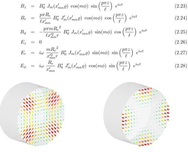
E0 is the amplitude of the electric field. B^∗₀ =B0/Jm(x⁰_m1) with B0 being the amplitude of the magnetic field. Jm(x) is the mth Bessel function of the first kind and J_m⁰ (x) is its first derivative withx_mn and x⁰_mn being the nth zero, respectively. %=r/R_c.

B_z = B₀^∗ J_m(x⁰_mn%) cos(mφ) sinpπz

`

e^iωt (2.23)

Br = pπRc

`x⁰_mn B₀^∗ J_m⁰ (x⁰_mn%) cos(mφ) cos pπz

`

e^iωt (2.24)

B_φ = −pπmRc2

`x⁰²_mnr B₀^∗ J_m(x⁰_mn%) sin(mφ) cospπz

`

e^iωt (2.25)

Ez = 0 (2.26)

Er = iω mRc2

x⁰²_mnr B₀^∗ Jm(x⁰_mn%) sin(mφ) sin pπz

`

e^iωt (2.27)

E_φ = iω R_c

x⁰_mn B₀^∗ J_m⁰ (x⁰_mn%) cos(mφ) sinpπz

`

e^iωt (2.28)

Figure 2.17: electric field of the TE₂₁₁ mode Figure 2.18: magnetic field of the TE₂₁₁mode

Figure 2.19: electric field of the TE mode Figure 2.20: magnetic field of the TE mode

(21)

2.3 RF Cavities [2] RF Resonators & Linac Structures

2.3 RF Cavities

In RF cavities, which usually have a cylindrical geometry, the basic pillbox modes as explained in the previous section are used to generate a longitudinal electric field along the beam axis.

While with TM modes the inherently present longitudinal electric field component can be used directly for particle acceleration like for example in case of elliptical pillbox cavities (section 2.3.1) or the Alvarez DTL (section 2.3.2), in TE mode cavities like the CH-structure (section 2.3.3) or IH-structure (section 2.3.4), an electric field in-between drift tubes is yielded by charging them using the actually perpendicular to the beam axis but parallel to the stems oriented electric field induced by the longitudinal magnetic field of the respective cavity mode.

Besides the cavity radius R_c and cavity length`(see Eq. 2.21 and Eq. 2.22), the geometry of the stems and drift tubes has a major influence on the resonance frequency mainly by affecting the overall capacitance. The actual field distribution is solely determined by the excited cavity mode.

Another important linac structure that is an RF cavity and not further mentioned is the 4-Vane- RFQ, in which the TE211 mode is utilized similar as in a CH-structure, in order to charge the respectively adjacent vane shaped electrodes with opposite polarity [27, p. 21 ff.].

2.3.1 Elliptical Pillbox Cavities

Figure 2.21:electric field distribution in a 5-cell elliptical pillbox cavity

Figure 2.22:magnetic field distribution in a 5-cell elliptical pillbox cavity Elliptical pillbox cavities, which are operated in the TM010 mode, are typically used with frequencies between 350 MHz and 3 GHz for the acceleration of particles with highly relativistic velocities like electrons withβ ≈1 or protons and ions withβ >0,5 [43, p. 175 ff.]. The elliptical variant of the pillbox shape provides a good suppression of multipacting and very low electric and magnetic peak fields, which allows high acceleration gradients. Often elliptical cavities are used in multi-cell structures operated inπ-mode like depicted in Fig. 2.21 and Fig. 2.22.

2.3.2 Alvarez DTL

The Alvarez drift tube linac (DTL) basically consists of a long cylindrical structure in which the TM010 cavity mode is excited. In addition drift tubes with a cut-off frequencyfc> f0 are fitted along the beam axis in order to shield the accelerated particles from the electric field during

(22)

[2] RF Resonators & Linac Structures 2.3 RF Cavities

the decelerating half of the RF period. Thus the time between the transitions of adjacent gap centers has to be the full duration of the RF cycle (0-mode) and the distance between the gap centers must be adapted gradually according to `_c = βλ. Since there is no transversal electric field component there is also no current on the retaining rods for the drift tubes that overall are uncharged at all times.

Figure 2.23: magnetic field distribution in an Alvarez DTL

Figure 2.24:electric field distribution between the drift tubes of an Alvarez DTL

2.3.3 CH-Structures

The ‘cross-bar’ H-mode (CH) structure is a drift tube linac that is operated with the TE₂₁₁ quadrupole mode (Fig. 2.17 and Fig. 2.18) and consists of a cylindrical cavity in which multiple (at least four) stems are mounted alternately rotated by 90^◦ like in a multi-spoke cavity (also see Fig. 6.5), thus achieving the electric charging of adjacent drift tubes with opposite polarity and

Figure 2.25: magnetic field distribution in a CH-structure

Figure 2.26: electric field distribution between the charged drift tubes of a CH-structure

(23)

2.3 RF Cavities [2] RF Resonators & Linac Structures

finally obtaining a longitudinal electric field component (in π-mode) like depicted in Fig. 2.26.

CH-structures are for a given frequency about twice the size in diameter compared to IH-structures and can thus be used with frequencies between 150 and 800 MHz while still having practicable transversal dimensions. The energy of the accelerated particles is usually between 1,5 and 150 MeV/u, corresponding to velocities of 0,05< β <0,5 [43, p. 173]. In TE mode cavities there is less magnetic field close to the conducting walls than in TM mode structures and there is also no longitudinal charging current on the cavity shell like in an Alvarez DTL. Therefore compar- atively high shunt impedances can be achieved, especially with structures for particles with low or medium energies (see [42, Fig. 4.5] or [14, Fig. 14]). The paths of the charging currents range over half the circumference in IH-cavities and over a quarter of it in CH-structures. In addition the possible implementation of the KONUS (german: ‘KOmbinierteNUll GradStruktur’) beam dynamics concept [49, p. 39 ff.] allows long acceleration sections with up to 20 gaps without interjacent magnetic lenses for transverse beam focusing, resulting in high average acceleration gradients. Because the cross-bar construction has a high mechanical stability and the sturdy stem design provides a good coolability, CH-structures are also well suited for superconducting applications. CH-cavities currently under development at IAP are 217-MHz CH-structures for the superconducting (sc) continuous wave (cw) linac project at GSI for the production of super heavy elements (SHE) ([12] and [31]), a superconducting 325-MHz CH-structure designed for the UNILAC at GSI [32] and a high gradient room temperature CH-cavity [3].

2.3.4 IH-Structures

The ‘interdigital’ H-mode (IH) structure is operated with the TE₁₁₁ dipole mode (Fig. 2.19 and Fig. 2.20) and contains open-ended stems that are alternately mounted to opposite sides of the cavity structure (Fig. 2.28). Typically IH-structures are used in the frequency range between 30 and 250 MHz, being limited to higher frequencies due to the decreasing transversal dimensions, and for particle energies between 120 keV/u and 7 MeV/u [42].

Figure 2.27: magnetic field distribution in an IH-structure

Figure 2.28: electric field distribution between the charged drift tubes of an IH-structure

(24)

[2] RF Resonators & Linac Structures 2.4 Resonator Parameters

2.4 Resonator Parameters

The overall performance of an accelerator structure is primarily characterised by its capability to transfer the injected RF power to the accelerated particle beam and is in general determined by the values of the generated acceleration voltageU0 (or U_eff) and the power loss Pc inside the cavity, from whom the commonly used resonator parameters for the comparison and description of different linac structures are derived.

2.4.1 Acceleration Voltage

Under harmonic excitation with frequencyf =ω/(2π) the electric field componentE_z(z, t) along the beam axis is given by Eq. 2.29, with Ez,max(z) being the amplitude atz.

Ez(z, t) =Ez,max(z) cos(ωt) (2.29) The acceleration voltage U₀ of an acceleration gap is defined as the voltage that an imaginary particle with infinite speed would traverse by passing the whole effective gap lengthgeff(Fig. 2.29) at the time t= 0 of the maximum field level [42, p. 26 f.].

U0 =

geff/2

Z

−g_eff/2

Ez,max(z)dz (2.30)

z g

Ez,max(z)

g_eff

Figure 2.29:gap geometry and exemplary field distribution ofE_z,max(z) [50, p. 33]

For numerical calculations on βλ/2-structures the effective gap length can be assumed asg_eff= βλ/2 becauseE_z,max(z)>0 around the center of the gap at z= 0 for −βλ/4< z < βλ/4.

The longitudinal electric fieldE_z(z, β) for a particle that moves along the beam axis with velocity β (which is assumed to be constant for

−g_eff/2 < z < g_eff/2) and reaches the center of the gap when E_z(z = 0, t) = E_z,max(z = 0) at t = 0 can be calculated from Eq. 2.29 by introducing t = z/βc. The traversed voltage U_eff is called effective voltage. Because U_eff is smaller than U0 the so called ‘transit time factor’T(β) =U_eff/U₀ is always smaller than 1.

U_eff=

geff/2

Z

−g_eff/2

E_z,max(z) cos(ωt) dz=

geff/2

Z

−g_eff/2

E_z,max(z) cos ωz

βc

dz =U₀ T(β) (2.31)

(25)

2.4 Resonator Parameters [2] RF Resonators & Linac Structures

For an accelerator structure with n gaps the sum over the individual acceleration voltages U0,n

and U_eff,n of each gap yields the total voltagesU0 =P

nU0,n and U_eff =P

nU_eff,n, respectively.

2.4.2 Quality Factor

The stored energyW inside a cavity can be calculated from Eq. 2.32 using the field distribution of either the maximum electric field E~_max(~x) or maximum magnetic fieldH~_max(~x) [42, p. 28].

W = 1 2µ₀

Z

V

|H~_max(~x)|² dV = 1 2₀

Z

V

|E~_max(~x)|² dV (2.32)

The ohmic power loss P_c due to induced eddy currents on the surface inside a cavity can be calculated from Eq. 2.33, where S is the entire resonator surface area and R_s is the surface resistance [42, p. 29]. At room temperature, Rs = 1/(σδ) depends on the conductivity σ of the material of the surface layer and on the current density distribution within. At the skin depth δ =p

2/(σωµ) inside the material the current density J(x) =J_se^−x/δcos(x/δ) is decreased due to the skin effect to 1/eof the current densityJs =J(x= 0) at the surface [42, p. 18 f.].

Pc= 1 2Rs

Z

S

|H~max(~x)|² dA (2.33)

The unloaded quality factorQ₀ as defined in Eq. 2.34 [50, p. 141 f.] is a measure to describe a resonator’s ability to store electromagnetic energy and is thus determined by the ratio of the stored energyW and the power lossP_c. If the power coupler of the resonator is being switched off at time t = 0, whenW(t = 0) = W and P_c(t= 0) = P_c, the power loss P_c(t) = −dW(t)/dt equals the rate of the overall energy dissipation [42, p. 89 ff.]. Therefore the stored energy at time tis given by W(t) =W(t= 0)·e^−t/τ with τ =Q₀/ω₀ (using Eq. 2.34) and Q₀ = 2πN equals the product of 2π and the number N of RF cycles at which the stored energy W(t=N f₀⁻¹) =W(t= 0)/e has reduced to 1/e of its initial value.

Q0 = ω0W

P_c (2.34) QL= ω0W

P_tot (2.35)

Because the energy dissipation Pc is related to the width ∆ω = 2(ω⁰−ω0) of the system’s resonance curve |A(ω)| (which is typically given by the Lorentz function stated in Eq. 2.37), the definition of Q₀ according to Eq. 2.36 is equivalent to Eq. 2.34 [42, p. 25]. |A(ω)| is the corresponding field amplitude and|A(ω⁰)|=|A(ω₀)|/√

2, so that for a quantityB(|A(ω)|²) with square dependence on |A(ω)|, ∆ω is the FWHM of B(ω).

Q0 = ω₀

∆ω (2.36) |A(ω)|= |A(ω₀)|

q

1 +Q02(∆ω/ω0)²

(2.37)

(26)

[2] RF Resonators & Linac Structures 2.4 Resonator Parameters

In an experimental setup it is not possible to analyzeP_cby itself because power is also dissipated through the power coupler (emitted powerPe) and the pick-up antenna (transmitted power Pt).

The loaded quality factor QL given by Eq. 2.35 includes the total power loss Ptot =Pc+Pe+Pt

[42, p. 90]. However,Q₀ can be calculated from the experimentally determined Q_L by assuming critical coupling, for which Q0 = 2·QL.

2.4.3 Shunt Impedance

Regarding its RF properties, an accelerator cavity can be treated similar to a parallel resonant circuit consisting of a capacitanceC, an inductanceL and a resistance Rp [42, p. 29 f.]. In case of resonance (ω = ω₀ = 1/√

LC), the impedance is equal to the value of R_p (Eq. 2.38), which provides a measure for the efficiency of a resonator. SubstitutingU0 withUeff yields the effective impedanceRa (Eq. 2.39).

R_p = U₀² Pc

= 2Q₀

ω0C (2.38) R_a = U_eff²

Pc

=R_pT² (2.39)

In order to compare accelerator structures of different lenght`, the shunt impedanceZ0(Eq. 2.40) and effective shunt impedance Z_a (Eq. 2.41) are used, which are R_p and R_a standardised to the structure length `, that is commonly defined as`=n(βλ/2) (nbeing the number of acceleration gaps) and is therefore not identical to the actual geometric length `⁰.

Z₀= R_p

` = U₀²

P_c` [Ω/m] (2.40) Z_a= R_a

` = U_eff²

P_c` =Z₀T² [Ω/m] (2.41)

2.4.4 Geometry Factor G & Geometric Impedance R_a/Q₀

The geometry factorG(Eq. 2.42) as standardised quality factorQ₀ and the geometric impedance R_a/Q₀ (Eq. 2.43) as standardised effective impedance R_a are independent of the frequency ω₀, the surface resistance Rs and the linear dimensions of the respective accelerator structure and hence characterise a resonator cavity under restriction to its geometry [42, p. 31 f.].

G=R_sQ₀ = R_sω₀W

P_c [Ω] (2.42) Ra/Q0 = Ueff2

ω0W = U02T²

ω0W [Ω] (2.43)

(27)

[3] Longitudinal Beam Dynamics & Phase Focusing

In RF drift tube linacs charged beam particles are accelerated by electric fields between oppositely poled charged drift tubes. The charge polarity of the tubes as well as the orientation of the electric fields in between has a periodic time dependence. Thus the accelerated beam has to consist of particle bunches whose transitions through the acceleration gaps have to be synchronous to the RF phase φ_rf in order to pass each gap when the electric field is oriented along the direction of motion of the bunch. Whereas a whole bunch is characterised by the phaseφs(relative toφrf) and energy Ws(z) of an imaginary particle called ‘synchronous particle’, individual bunch-particles with total energyW(z) and phaseφ(z) are described by the difference of energy ∆W(z) (Eq. 3.3) and difference of phase ∆φ(z) (Eq. 3.4) to the synchronous particle. Ws(z) as well asφsare set by the overall beam dynamics concept of the respective accelerator. ∆W(z) and ∆φ(z) constitute the phase space of the longitudinal particle motion.

3.1 Phase Stability

The change of energy dW(z)/dz and phase dφ(z)/dz for an on-axis particle (x = y = 0, x⁰ = dx/dz =y⁰ = dy/dz = 0) with charge q, velocity β(z) and phase φ(z) at a placez ist given by Eq. 3.1 and Eq. 3.2, respectively [26, p. 27 ff.].

dW(z)

dz =q Ez(z, φ(z)) =q Ez,max(z) cos(φ(z)) (3.1) dφ(z)

dz = ω0

β(z)c (3.2)

As aforementioned the position in the longitudinal phase space of a particle with energy W(z) and phaseφ(z) is given by Eq. 3.3 and Eq. 3.4 [16, p. 311]:

∆W(z) =W(z)−W_s(z) (3.3) ∆φ(z) =φ(z)−φ_s (3.4) Introducing Eq. 3.3 into Eq. 3.1 and Eq. 3.4 into Eq. 3.2 yields Eq. 3.5 and Eq. 3.6. For Eq. 3.6 the difference of relativistic kinetic energy ∆W(z) =m0c²γs(z)³βs(z)∆β(z) with ∆β(z) =β(z)−β_s(z) as well as the assumption ∆β(z)<<1 is employed [49, p. 13].

d(∆W(z))

dz =q E_z,max(z) cos(φ_s+ ∆φ(z))−cos(φ_s)

=−∂H(∆W(z),∆φ(z))

∂(∆φ(z)) (3.5)

(28)

[3] Longitudinal Beam Dynamics & Phase Focusing 3.1 Phase Stability

d(∆φ(z)) dz = ω0

c 1

β(z) − 1 β_s(z)

=− ω0∆W(z)

m₀c³γ_s(z)³β_s(z)³ = ∂H(∆W(z),∆φ(z))

∂(∆W(z)) (3.6)

Integration of Eq. 3.5 over ∆φ(z) and Eq. 3.6 over ∆W(z) leads to the Hamilton function H(z) for the longitudinal particle motion (Eq. 3.7). Setting H(z) to a constant value C =Hconst and solving Eq. 3.7 for ∆W(∆φ(z)) yields Eq. 3.8 from which (assuming γs(z)βs(z) = const. and choosing E_z,max(z) = const. = U_eff/g_eff) the phase space trajectories shown in Fig. 3.1, Fig. 3.3 and Fig. 3.5 can be calculated¹.

H(∆W(z),∆φ(z)) =− ω0

m₀c³γ_s(z)³β_s(z)³

∆W(z)² 2

−q Ez,max(z) sin(φs+ ∆φ(z))−(φs+ ∆φ(z)) cos(φs)

(3.7)

∆W(∆φ(z)) =± s

2m₀(cγ_sβ_s)³ ω0

qU_eff

geff

(φ_s+ ∆φ(z)) cos(φ_s)−sin(φ_s+ ∆φ(z))

−C

(3.8)

-40 -30 -20 -10 0 10 20 30 40 50 60

-0,10 -0,08 -0,06 -0,04 -0,02 0,00 0,02 0,04 0,06 0,08 0,10

∆W / Ws

∆φϕ[°]

Figure 3.1: ∆W(∆φ)/W_s forφ_s= 0 and various values ofC=H_const

-90 -60 -30 0 30 60 90

E_z,max

[°]

ϕ

0

Ez(ϕ)

Figure 3.2:Ez(φ) aroundφs= 0 (blue dot: synchronous particle) Forφ_s= 0 the total acceleration voltageU_s(Eq. 3.9) for the synchronous particle equalsU_eff (see Eq. 2.31). Particles that arrive at z prior to it (φ < φ_s, green dot - Fig. 3.2) experience a lower electric field level and therefore approach it longitudinally as the bunch moves along the beam axis. However, particles that arrive after the synchronous particle (φ > φ_s, red dot - Fig. 3.2) also see a lower field and are unable to catch up. Hence the particle bunch as a whole is unstable and will disintegrate during the acceleration process (also see Fig. 3.1). For lower values of φs

(−90^◦ < φ_s < 0) the achieved acceleration voltage U_s(φ_s) < U_eff decreases. Like in the case of φ_s = 0, particles with φ < φ_s (green dot - Fig. 3.4) move towards the synchronous particle because of the lower energy gain. On the contrary particles that arrive at z at a later time with