Bone material characteristics influenced by osteocytes

(1)

Bone Material Characteristics Influenced by Osteocytes

D i s s e r t a t i o n

zur Erlangung des akademischen Grades d o c t o r r e r u m n a t u r a l i u m

(Dr. rer. nat.) im Fach Physik

eingereicht an der

Mathematisch-Naturwissenschaftlichen Fakultät I der Humboldt-Universität zu Berlin

von

Diplom Physiker Michael Kerschnitzki

Präsident der Humboldt-Universität zu Berlin:

Prof. Dr. Jan-Hendrik Olbertz

Dekan der Mathematisch-Naturwissenschaftlichen Fakultät I:

Prof. Dr. Andreas Herrmann

Gutachter/innen: 1. Prof. Dr. Dr. h.c. Peter Fratzl 2. Prof. Dr. Franz Pfeiffer

3. Prof. Dr. Norbert Koch

Tag der mündlichen Prüfung: 24.02.2012

(2)

(3)

Kurzfassung

In dieser Doktorarbeit wird die Hypothese geprüft, ob Osteozyten einen direkten Einfluss auf die Knocheneigenschaften in ihrer unmittelbaren Umgebung haben.

Der zentrale Experimentieransatz ist dabei die Korrelation der Organisation des Osteozytennetzwerks mit den Mineraleigenschaften des Knochens auf der Sub- mikrometerebene. Es wird gezeigt, dass bereits die anfängliche Ausrichtung der Osteoblasten entscheidend für die Synthese von hoch ausgerichtetem Knochen- material ist. Die dabei entstehenden Osteozytennetzwerke sind so organisiert, dass die Osteozyten und ihre Zellfortsätze jeweils einen möglichst kleinen Ab- stand zum Knochenmineral haben. Deshalb wird vermutet, dass genau diese Netzwerkorganisation mitentscheidend ist, wie gut die Zellen das Mineral in ihrer Umgebung beeinflussen können. Messungen der Knochenmineraleigenschaf- ten auf Submikrometerebene mit Röntgenkleinwinkelstreuung bestätigen diese Vermutung. Dabei wird deutlich, dass Knochenmaterial in der Nähe der Osteozy- ten durch andere Mineraleigenschaften geprägt ist. Um zu klären, wie Osteozyten Mineral in ihrer direkten Umgebung verändern können, werden Mechanismen der passiven Mineralherauslösung aus der mineralisierten Oberfläche des Osteo- zytennetzwerks untersucht. Es wird gezeigt, dass kalziumarme ionische Lösun- gen unter physiologischen Bedingungen große Mengen von Kalzium-Ionen aus dem Knochen lösen und diese dann durch die Osteozytennetzwerkstrukturen diffundieren können. Zum Abschluss wurde medullärer Knochen von Hühnern als ein Modellsystem für rasanten Knochenumbau untersucht. Dieser spezielle Knochentyp dient den Hennen als labiles Kalziumreservoir und ermöglicht da- durch die tägliche Eierschalenproduktion. Experimente am medullären Knochen- material zeigen insbesondere die Bedeutung von weniger stabilen Mineralstruk- turen die benötigt werden um den Knochen an den schnellen, sich wiederholenden Knochenauf- sowie Abbau optimal anzupassen.

Knochenaufbau, Osteozytennetzwerke, Osteozytische Osteolyse, Klein- winkelstreuung, Konfokale Mikroskopie

(4)

(5)

Abstract

This thesis aims to test the hypothesis whether osteocytes have a direct influence on bone material properties in their vicinity. In this regard, the concomitant analysis of osteocyte network organization and bone ultrastructural properties on the submicron level is the central approach to answer this question. In this work, it is shown that already initial cell-cell alignment during the process of bone formation is crucial for the synthesis of highly organized bone. Furthermore it is proposed that the occurrence of highly ordered osteocyte networks visualized with confocal laser scanning microscopy (CLSM) has a strong impact on the ability of osteocytes to directly influence bone material properties. These highly organized networks are another consequence of initial cell-cell alignment and are found to be arranged such as to feature short mineral cell distances. Examination of submicron mineral properties with scanning small angle x-ray scattering (sSAXS) shows that bone material in the direct vicinity of osteocytes and their cell processes shows different mineral properties compared to bone further away in the depth of the tissue. Moreover, mechanisms of passive mineral extraction from the mineralized surface of the osteocyte network, due to the treatment with calcium poor ionic solutions, are investigated. It is shown that this chemical process oc- curring under physiological conditions leads not only to the dissolution of con- siderable amounts of calcium, but also to efficient diffusion of these ions through the osteocyte network structures. Finally, medullary bone which is intended as a labile calcium source for daily egg shell formation in hens is used as a model system for rapid bone turnover rates. This bone type in particular indicates the importance of uniquely adapted, less stable mineral structures to fit the requirements for rapid bone resorption as well as re-formation.

Bone formation, osteocyte networks, osteocytic osteolysis, small angle x- ray scattering (SAXS), confocal laser scanning microscopy (CLSM)

(6)

(7)

(8)

1 Introduction

Bone is one of the most intensively studied biological materials, composed from inorganic hydroxyapatite mineral crystals which are embedded in an organic extracellular collagen matrix. Bone features several levels of hierarchy, which together involve unique implications on macroscopic bone material properties (Weiner and Wagner 1998; Currey 2002; Fratzl and Weinkamer 2007). Further- more bone is the main mineral reservoir for maintaining body calcium and phosphate homeostasis (Aarden, Burger et al. 1994; Bonewald 2007). A detailed understanding of the dynamic processes of bone formation and remodeling during physiological growth, healing and aging as well as in the case of pathological cases of bone diseases has high clinical relevance. Bone development and adaptation involves not only various cellular interactions (Cowin 2004; Chen, Liu et al. 2010) but also depends on dynamic chemical processes of bone mineral crys- tallization (Weiner and Traub 1992; Landis 1995; Olszta, Cheng et al. 2007).

Thus, bone research is a highly interdisciplinary field at the interface of medi- cine, chemistry, biology and material science.

Bone remodeling is traditionally attributed to osteoblasts and osteoclasts – cells which deposit and resorb bone, respectively (Buckwalter, Glimcher et al. 1995).

These cells are also the primary target of treatments against bone diseases leading to an imbalance of bone formation and resorption and thus to substantially decreased bone quality (Rodan and Martin 2000; Roschger, Paschalis et al.

2008). Osteocytes are the cells residing within the bone matrix, deriving from osteoblasts which get embedded during the process of bone deposition (Franz- Odendaal, Hall et al. 2006) and create a network of extracellular spaces by which the bone tissue is perfused (Lanyon, Rubin et al. 1993). Osteocytes are known to orchestrate the delicate activity of osteoclasts and osteoblasts (Burger and Klein- Nulend 1999; Bonewald and Johnson 2008; Nakashima, Hayashi et al. 2011).

However, to date more evidence arises, that osteocytes are also directly involved in bone mineral homeostasis. The surface area of the osteocyte network can be estimated 100 fold greater than the surface available to osteoblasts and osteoclasts (Aarden, Burger et al. 1994; Teti and Zallone 2009). Therefore, it seems possible that osteocytes may act directly on the bone material they are in contact

(12)

with, having some ability to deposit and resorb mineral (Bonewald 2007; Bonu- cci 2009; Teti and Zallone 2009) and thus directly control bone quality as well as fragility.

1.1 Scope and Aims of the Work

In this PhD thesis, the hypothesis will be tested whether osteocytes directly influence bone material in their vicinity. This implies that bone material adjacent to osteocytes and their cell processes could be more dynamic and thus, may have a different structure as compared to bone further away in the bulk of the tissue. The chosen approach to solve this complex problem is a combination of techniques to reveal osteocyte network organization together with the measurement of bone ultrastructural properties on the submicron level. This concomitant analysis offers the possibility to better understand the influence of cell-cell organization during the dynamic processes of bone formation and remodeling as well as the possibility of cell-matrix interactions – with particular regard to osteocytes. This will improve the understanding of the impact of osteocyte network organization in conjunction with osteocyte activity on bone tissue characteristics such as matrix orientation and mineralization. As these factors mainly influence bone quality as well as bone fragility, these new insights can help to better understand the role of osteocytes during calcium and phosphate homeostasis. Furthermore, these insights may clarify whether these cells should be considered more urgently as a target for drug development in the context of bone diseases featuring deficient bone mineral homeostasis, such as osteoporosis.

The work is based on five different experimental steps: (i) Confocal laser scanning microscopy (CLSM) combined with rhodamine staining which allows the three-dimensional visualization of osteocyte networks in undemineralized bone sections. Furthermore, experimental procedures are developed to accommodate the assessment of bone material properties at the same location with various techniques such as back-scattered electron microscopy (BSE) and scanning small angle x-ray scattering (sSAXS). (ii) Subsequently, osteocyte network organization is visualized and correlated with bone tissue characteristics in different bone types from different species in order to better understand common geometries of the osteocyte network arrangement in conjunction with the surrounding bone

(13)

matrix. Moreover, implications on the dynamic processes of bone formation, bone healing and remodeling are made as osteocyte networks show the direct location of former osteoblasts during the process of bone deposition. (iii) To test whether bone material in the direct vicinity of the osteocytes and their cell processes shows different characteristics, high resolution sSAXS techniques are used to measure submicron bone mineral properties which are further correlated to the organization of the osteocyte networks. (iv) To further understand how osteocytes could modify bone mineral properties in their vicinity, passive mineral extraction from the mineralized surfaces exposed within the osteocyte network is performed. These experiments show the proposed potential of calcium ion dissolution and successive transportation through the osteocyte network structures. (v) Finally, medullary bone of egg laying chicken is investigated to better understand the requirements on bone material uniquely adapted for bone resorption as well as re-formation.

1.2 Outline of the Thesis

The thesis starts with a brief introduction, distinguishing between bone as a material and a living tissue. Firstly bone hierarchy and individual structural characteristics of different bone types will be explained, but also the main bone cells which control bone formation and remodeling will be introduced. This section is followed by the 3^rd chapter briefly introducing the theoretical background of physical methods used, focusing on confocal laser scanning microscopy, electron microscopy and small angle x-ray scattering. In the 4^th chapter initial preparation of bone samples as well as experimental setups are explained. A detailed description of all methods and sample preparation protocols especially developed during this PhD-project can be found in the 5^th chapter. In the 6^th chapter, experimental findings are discussed in detail, followed by general conclusions and a perspec- tive for future research in the 7^th chapter.

(14)

(15)

2 Bone and Bone Mineral

Bone is the main component forming the skeletal system in all vertebrates. The human skeleton consists of approximately 206 different bones, individually in shape, size and mechanical properties, depending on their anatomical position and function. As an example, the skull must be flexible during stages of growth but still protective to prevent external impacts on the brain, whereas auditory ossicles residing inside the ear are, due to acoustical reasons, stiff and brittle (Currey 2003). Additionally to their multifunctionality, bones continuously adjust to external stimuli by remodeling, performed by coordinated interactions of bone cells (Duncan and Turner 1995). Thus bone is not only a static material but continuously undergoes adaptation throughout its whole lifecycle (Frost 1987; Cur- rey 2003; Fratzl and Weinkamer 2007). In the following these two approaches to firstly understand bone as a ‘static material’ but also secondly as a living organ- ism, will be described.

2.1 Bone as a Material

Bone material features a complex hierarchical structure ranging over several levels of hierarchy from the molecular- up to the macroscopic level (Rho, Kuhn- Spearing et al. 1998; Weiner and Wagner 1998; Currey 2002; Fratzl and Weink- amer 2007). At lowest levels of hierarchy bone is a nano composite formed from collagen type 1 molecules and carbonated hydroxyapatite mineral particles (Fratzl, Gupta et al. 2004). Triple helical collagen molecules self-assemble to approximately 100 nm thick fibrils in such way, that adjacent collagen molecules are staggered in axial direction by 67 nm leading to banded structures showing the characteristic gap and overlap zones (Petruska and Hodge 1964; Landis, Hodgens et al. 1996). Collagen fibrils are mineralized with carbonated hydroxyapatite mineral crystals. It was reported that nucleation of those starts in the gap regions (Landis, Hodgens et al. 1996; Landis, Hodgens et al. 1996) however a recent report states a initiation of mineral nucleation in the overlap zone (Nudelman, Pieterse et al. 2010) with further growth to flat plate-like crystals (Weiner and Traub 1992; Landis, Hodgens et al. 1996). Water is the third major component at lowest levels of hierarchy located within and between the fibrils

(16)

and collagen molecules. During processes of mineralization, water is partly sub- stituted with bone mineral (Fratzl, Fratzl-Zelman et al. 1993).

Mineralized collagen fibrils further assemble to fibrillar arrays building up di- verse organizational patterns which can be generalized to 4 different bone types (Weiner and Wagner 1998): (i) Parallel-fibered bone features arrays of collagen fibrils arranged in a parallel manner over ranges of micrometers and even milli- meters. This type of bone is very rapidly formed and usually can be found in ten- dons, skeleton of fish, amphibians and the bovid family. Opposing to parallel fibered bone (ii) woven fibered bone is characterized by no long range order.

Fibrils are arranged to poorly oriented and loosely packed bundles with diameters up to 30 µm. Woven bone forms and mineralizes very rapidly but only offers poor mechanical properties. It is found to be the first deposited bone type after fractures and during early stages of embryonic development and subsequently gets replaced by other bone types. (iii) Plywood-like structures feature sets of parallel fibrils arranged in layers, with alternating fibril orientation between individual layers. Lamellar bone as one example of twisted plywood-like structures is very often found in mammals centrically arranged around the Haversian canal containing the blood vessel. It features excellent mechanical properties and is formed at lower rates as compared to parallel-fibered or woven bone. (iv) An- other structural motif of fibrillar arrays is the radial fibril orientation, characteristic for the inner layer of teeth. Fibrils are aligned in plane, radial to the surface of the tubule present in the bulk of dentin (Figure 1).

Figure 1: Scheme of the 4 different bone types: (a) parallel fibred bone, (b) woven bone, (c) plywood-like lamellar bone and (d) radial fibril orientation. Adapted from (Weiner and Wagner 1998).

In larger mammals, in particular in cattle, fibrolamellar bone can be found (Currey 2002; Mori, Kodaka et al. 2003; Mori, Hirayama et al. 2007). This bone

(17)

type features a mixture of poorly aligned, rapidly growing woven bone and highly aligned parallel-fibered or lamellar bone. This structural composition is beneficial as these animals have to grow fast but still, bones need to withstand high mechanical loading.

At the next hierarchical level, the structure of bone is distinguished in compact cortical and spongy trabecular bone. Cortical bone forms the outer bone shell and is characterized by low porosity (< 10 %), which is mainly due to the occurrence of blood vessels and cellular spaces which also can act as initiation points for cracks (Nicolella, Bonewald et al. 2005; Nicolella, Moravits et al. 2006; Ebacher and Wang 2009). Whereas human cortical bone is composed of numerous osteons ensuring good blood supply, cortical bone in cattle and horses is mainly composed of fibrolamellar bone featuring less supply with blood, which leads to longer healing times in case of fracture. In areas of heavy compressive loading such as the head of the femur or the vertebrae, the cortical bone shell is filled with spongeous trabecular bone featuring high porosity (> 80 %). The individual lamellar bone struts with a diameter ranging between 100 and 300 µm are not supplied with blood as nutrition of bone cells is assured by the surrounding bone marrow.

On the macroscopic level, shapes of bones range from long bones like the femur which provide stability against bending and buckling, over flat bones as the scapula to block-shaped or plate-shaped bones as the vertebrae or skull providing stability against bending as well as protecting vital organs.

The complex hierarchical structure of bone has several implications for bone mechanics as every level of hierarchy contributes to macroscopic mechanical properties of the bone material. Just to mention some examples, in literature it is suggested that at the nano-scale, strong mechanical heterogeneity accounts for crucial mechanisms of energy dissipation during mechanical loading (Tai, Dao et al. 2007). In this regard, inorganic mineral particles provide stiffness but also being shielded from strong deformation by the ductile organic collagen matrix which takes up the deformation energy by shearing (Jager and Fratzl 2000;

Gupta, Wagermaier et al. 2005; Gupta, Seto et al. 2006). However, also at higher levels of hierarchy, mechanisms of crack deflection at microscopic interfaces can

(18)

dissipate deformation energy (Peterlik, Roschger et al. 2006; Koester, Ager et al.

2008).

2.2 Bone as a Living Tissue

Bone is a dynamic living tissue as it features the unique ability not to be only statistically predefined by its genetic blueprint. Furthermore it is able to continuously adapt to changing external biophysical stimuli of its environment to improve functionality (Thompson 1992; Fratzl and Weinkamer 2007; Meyers, Chen et al. 2008). Even without a change in stimulus, dynamic self-healing mechanisms continuously remediate damage and thus strengthen the bone material.

In bone the ability of adaption derives from permanent processes of remodeling of the entire bone material. Remodeling is beneficial as it (i) increases the blood supply, (ii) removes dead bone, (iii) takes out microcracks, (iv) changes the grain which leads to improved mechanical properties and (v) contributes to body mineral homeostasis (Currey 2002). Processes of remodeling are a consequence of interplay of the bone cells. Osteoclasts resorb bone leaving small cavities. Os- teoblasts subsequently fill those with new, completely unmineralized bone material. Subsequent mineralization of the newly deposited material is very rapid during the first days – reaching about 50 % of the final degree of mineralization – followed by a phase of continuous slow mineralization leading to a permanent increase in mineral content (Fratzl, Gupta et al. 2004; Ruffoni, Fratzl et al. 2008).

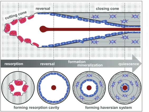
In trabecular bone, due to its high surface to volume ratio, osteoclasts have ac- cess to the whole bone volume just by resorbing cavities of approximately 60 µm (Jee 2001). Whereas in compact cortical bone (low surface to volume ratio), osteoclasts resorb a tunnel with a speed of approximately 20 – 40 µm/day (Jee 2001). These remaining tunnels get later filled with new lamellar bone material deposited by osteoblasts – forming a new haversian system also called secondary osteon which improves blood supply (Figure 2). Secondary osteons are separated from their surrounding older bone material by an impermeable cement line acting as an outer border. Thus, cells residing in the old bone are not supplied from the blood vessel anymore leading to cell death. Hence, in these areas the rate of formation of new secondary osteons is increased (Currey 2002).

(19)

cutting cone

reversal closing cone

forming resorption cavity forming haversian system reversal

resorption formationmineralization quiescence

Figure 2: Scheme of the formation of a secondary osteon in cortical bone. During resorption phase, osteoclasts in the cutting cone build a tunnel, which is followed by the reversal phase at which osteoblasts align at the surface of the resorbed cavity to subsequently deposit new lamellar bone material. After closure of the cone, remaining osteoblasts at the surface go to quiescence. Adapted from (Stroncek and Reichert 2008)

During the deposition of new bone, some osteoblasts get buried within the bone matrix and differentiate to osteocytes (Franz-Odendaal, Hall et al. 2006;

Nicolella, Moravits et al. 2006). Osteocytes reside inside their cell lacuna within the bulk of the bone material and are interconnected mutually as well as with the bone cells acting at the bone surface (Aarden, Burger et al. 1994; Marotti 2000;

Palumbo, Ferretti et al. 2004; Bonewald and Johnson 2008). In recent reviews osteocytes are often called to be ‘multifunctional’, ‘smart’ or even ‘amazing’

cells (Bonewald 2007; Bonewald 2011). Source of this nomenclature is the still remaining lack of knowledge of the particular role of this cell-type during bone homeostasis. Osteocytes are known to orchestrate bone remodeling in response to mechanical and microenvironmental changes as they have the capability to sense strain rates in their surrounding bone matrix (Klein-Nulend, Vanderplas et al. 1995; Burger and Klein-Nulend 1999; Bonewald and Johnson 2008). This

(20)

mechanosensation either occurs over direct straining of the cell (Nicolella, Mo- ravits et al. 2006), or via the detection of flow of interstitial fluid as a result of mechanical loading (Weinbaum, Cowin et al. 1994; Zeng, Cowin et al. 1994;

Owan, Burr et al. 1997).

Moreover, osteocytes have long been suspected to play a direct role in bone mineral homeostasis. The surface of the osteocyte network is estimated to be 100 fold greater than that of trabecular bone and even 400 fold greater than all the surfaces of the haversian systems in compact bone – thus surfaces typically available to osteoclasts and osteoblasts (Qing and Bonewald 2009; Teti and Zal- lone 2009). This leads to the conclusion that osteocytes, facing this enormous surface could potentially contribute to bone mineral homeostasis as they have some ability to deposit and resorb mineral in their vicinity (Baud 1962; Belanger 1969; Baylink, Wergedal et al. 1971; Parfitt 2003; Teti and Zallone 2009). Recep- tors for calcium regulating hormones (Boivin, Mesguich et al. 1987; Vanderplas and Nijweide 1988) as well as ion channels for the control of calcium and phosphate levels (Ravesloot, Vanhouten et al. 1990; Ravesloot, Vanhouten et al. 1991;

Teti and Zallone 2009; Bonewald 2011) could be found in osteocytes. Further- more the existence of molecules regulating mineralization such as Dmp1 (Toyosawa, Shintani et al. 2001) and sclerostin (van Bezooijen, Roelen et al.

2004; Gardner, van Bezooijen et al. 2005; Poole, van Bezooijen et al. 2005) were detected, implying that osteocytes are not only capable of controlling ionic con- centrations in their vicinity but also directly influence mineralization of the bone material they are facing (Baylink, Wergedal et al. 1971; Lane, Yao et al. 2006).

This further implies that mineral and the matrix in the neighborhood of osteocytes and their cell processes must be more dynamic and thus may have a different structure compared to bone further away in the depth of the tissue (Belanger 1969). In this sense it was proposed that a thin layer of amorphous or highly crystalline mineral is present at the surface of each osteocyte lacuna, which acts as a small mineral reservoir, being formed – and as needed – resorbed by the osteocyte (Bonucci 1990; Bonucci 2009). However, to reveal these modest mor- phological and ultrastructural changes of the bone material residing in the vicinity of osteocytes, a combination of sophisticated experimental techniques are needed which are capable of mapping bone material properties as a function of the distance to these cells.

(21)

3 Theoretical Background of Physical Methods Used

In this PhD-thesis, experimental techniques were applied to study osteocyte network morphologies and correlate these with bone ultrastructure at the micron- and the submicron scale. For this purpose confocal laser scanning microscopy – to measure osteocyte network organization – scanning electron microscopy – to further qualitatively measure bone mineralization – and small angle x-ray scattering – to determine submicron mineral characteristics – were used. In this chapter, the theoretical background of these physical methods is briefly introduced. Fur- ther information on the mutual accommodation of these complementary methods can be found in the following chapter 4 – Materials and Methods and 5 – Devel- opment of Experimental Procedures.

3.1 Confocal Laser Scanning Microscopy

In conventional light microscopy, image quality strongly depends on the thickness of the illuminated sample, as light coming from scattering objects above and below the focal plane reduces image contrast. Confocal microscopy is designed to remove obscuring out-of-focus light which further leads to an increase of lat- eral resolution (Price and Jerome 2011). In the confocal microscope light is focused to a defined point within the specimen. Light emerging from this defined point is further collected and focused by the objective lens to a spot at the image plane. Light arising from out-of-focus areas within the sample is focused differ- ently from the objective lens. This stray light is rejected by a small pinhole aperture which only allows light coming from the focal point to further pass towards the detector (Minsky 1988). A single point alone does not provide much information of the specimen. Thus, image information within the focal plane is collected sequentially by scanning the spot across. Confocal laser scanning microscopes (CLSM) utilize lasers as the luminous source. Here exhibition can be performed in transmission as well as in reflection mode in which fluorescent samples can be observed. Fluorescence imaging in reflection mode has the big advantage to provide a high contrast signal to maximally exploit the ability to remove out-of- focus light from the image (Price and Jerome 2011). For this purpose the excitation light which only gets reflected at the specimen and emission light arising

(22)

from the fluorescent characteristics of the sample is separated by appropriate filters only allowing certain defined wavelengths to pass.

Figure 3: Principle design of a confocal microscope. Light from the photon source is fo- cused at the first entrance pinhole, collected by the condenser lens and focused to the sam- ple. Light emerging from this focal plane is further collected by the objective lens and fo- cused at a second exit pinhole. Entrance, focal sample plane and exit pinhole are in conjugate focus (red lines). Light further reaches an emission filter only allowing a certain range of wavelengths to pass to the detector. Light emerging from out-of-focus planes (blue and green lines) is not transmitted to the detector as it reaches the exit pinhole out of focus.

Adapted from (Price and Jerome 2011).

In confocal laser scanning microscopy, either auto fluorescent materials or non- fluorescent materials which get specifically stained with fluorescent molecules (fluorochromes) can be measured in reflection mode. Here the fluorochromes absorb photons with a specific energy respectively wavelength (fluorochrome excitation). During this excitation the fluorochrome molecules undergo an electronic transition to a higher electronic state for which a certain amount of energy is required. In this regard only energies close to the excitation energy are absorbed by the fluorochromes thus offering specificity to the process of fluorescence. This specificity of certain staining media can be used due to utilization of different exciting lasers during the fluorescence measurement. After excitation, the molecule relaxes to lower vibration states within the electronic state before it eventually goes back to the ground state by generation of a photon. During the internal conversion of vibration relaxation, the energy is transferred in non- photon-generating reactions, mainly in the form of heat. This loss of energy leads to the generation of lower energy photons, respectively an increase in wavelength of the emissive light, which is called Stokes shift. Confocal microscopy benefits from this shift to longer wavelengths as it allows filtering the excitation from the

(23)

emissive light. Hence, final images only contain fluorescence information providing high contrasts.

Figure 4: (a) Jablonski diagram showing the excitation of a molecule due to absorption of an incident photon with the energy EP from the S0 to the S1 state with ΔEa = EP. Subsequent relaxation from S1 to S0 with emission of a photon with the energy Ee predominantly occurs after nonradiative processes of internal relaxation which leads to a loss of energy (ΔEa = ΔEe). (b) Schematic plot showing the excitation and emission spectra. These are not discrete since excitation and emission can occurs from and to different vibration states within dis- tinct electronic states. Due to separation of individual excitation and emission spectra, emit- ted light can be easily distinguished from incident light.

Excited molecules not only loose energy by emitting light. There are also other competing processes leading to relaxation to the ground state such as heat generation and energy transfer to neighboring molecules. These alternative nonradiative processes can decrease the amount of fluorescence and lead to worse imaging quality. The attribute of each fluorochrome to convert absorbed photons in fluorescence emission is specified by the quantum yield.

nr f

f

k k

k absorbed

photons

emitted photons

QY = = +

,

#

,

#

(Price and Jerome 2011) with QY as the quantum yield, kf as the rate of fluorescence and knr as the rate of all other nonradiative processes. A perfect emitter would feature QY = 1, emitting one photon of lower energy for each photon absorbed and thus assure strong fluorescence signals even at focal planes deep

(24)

inside the specimen. In bone, specific staining of bone cells or cavities within the bone material can be used to visualize long range organization of the material.

Due to the requirement of low transparency of the material and high penetration depths of the measurement (Schneider, Meier et al. 2010), staining with fluorochromes having a high quantum yield is necessary.

3.2 Back-scattered Electron Imaging

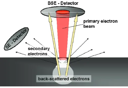
In opposition to conventional light microscopy techniques, scanning electron microscopy allows to examine samples in scanning mode by utilizing a focused electron beam. During measurement, interactions of the electrons with the specimen lead to processes of elastic and inelastic scattering accounting for back- scattered- as well as the generation of secondary electrons, respectively (Boyde and Jones 1996). During elastic scattering the energy of the electrons remain un- changed, only the trajectories of flight are affected. As a consequence a portion of the incoming electrons is scattered backwards. The amount of back-scattered electrons (BE) carries information on the atomic composition of the target area (Roschger, Plenk et al. 1995). During processes of inelastic scattering the energy of the electrons is altered due to several interactions with the sample leading – amongst other processes – to the generation of secondary electrons (SE). Secon- dary electrons show lower energies as compared to the primary beam energy.

Due to high attenuation of low energy electrons in matter, SEs reaching the detector originate only from a thin layer at the surface of the sample. As a consequence, detection of secondary electrons provides topographical information of the target area, as surfaces have strong impact on the SE-signal (Koshikaw.T and Shimizu 1974).

(25)

Figure 5: Scheme depicting the origin of the two different signals measured with scanning electron microscopy. Secondary electrons (SE) are generated due to inelastic scattering events between the primary electron beam and the material. Due to strong reabsorption of SE, only those generated within a thin layer at the surface can escape the material. Back- scattered electrons (BSE) are a result of elastic scattering events. The amount of back- scattered electrons carries information on the atomic composition of the material. Adapted from (Johnson 1990).

In bone tissue calcium atoms have the highest atomic number (Z = 20) and consequently dominate the BE-signal. Thus back-scattered electrons can be used to measure the local calcium concentration, respectively the degree of mineralization – also an indication for bone age (see chapter 2.2) – which can additionally give useful implications on bone growth and remodeling dynamics (Roschger, Paschalis et al. 2008).

3.3 Small Angle X-ray Scattering

X-rays as electromagnetic waves interact with matter by means of absorption as well as elastic and inelastic scattering. Processes of absorption, involving subsequent processes of fluorescence, can be used for elemental analysis as well as for the structural studies such as radiography. Processes of elastic scattering provide information on the submicron structure of the examined material. Commonly it is distinguished between x-ray scattering which is a result of elastic interactions between waves (or photons) and a material without long range order (no regular arrangement of atoms) and x-ray diffraction as a result of elastic interaction with

(26)

materials featuring long range order (regular arrangement of atoms) and thus leading to characteristic patterns of interference behind the illuminated object.

In this thesis, small angle x-ray scattering (SAXS) was one of the main experimental techniques. SAXS is a diffuse elastic scattering up to angles of 5° describing randomly oriented systems containing two phases with different electron densities with sharp interfaces (Kratky, Porod et al. 1951; Porod 1951; Porod 1952) in the range from 1nm up to 1 µm. In bone, two phases are represented by the collagen phase with low electron density and the mineral phase with high electron density. Information on the size, orientation and shape of submicron mineral particles can be derived from the scattering intensity distribution I(qr)

2

) 3

exp(

) ( )

( r iqr d r

V q K I

V

r r r

r =

∫

^ρ ⋅

with qr as the scattering vector (Figure 6), V as the sample volume and K as an instrumental constant. The scattering vector qr is defined to be the difference of the wave vector of the scattered beam kr'

and the wave vector of the incident beam with kr

λ π^/ 2 ' =

= k kr r

for elastic scattering. Accordingly, the modulus of qr can be derived from

λ θ θ ⁴π ^sin sin

2 ⋅ =

= k qr

Furthermore, Porod’s law states that in systems containing two phases of different mean electron densities, separated with sharp interfaces, the following equation is valid for large q values:

) 4

( q

q P

I ⎯^q⎯ →^→⎯^∞

(27)

with P as the Porod constant calculated from the Porod-plot (see chapter 4.3.2) and B as the background. This equation points out that in all biphasic systems with distinct interfaces the scattering intensity decreases with q^-4.

Figure 6: Scheme of SAXS scattering: the scattering vector q is calculated from the incom- ing wave vector k and the scattered wave vector k’. 2θ is the scattering angle between k and k’.

Whereas the degree of mineral particle orientation is obtained from the two- dimensional shape of the SAXS-scattering signal (see chapter 4.3.2 for azimuthal integration), information on the mean mineral particle thickness (T-parameter) can be derived from the decay of the scattering signal with larger scattering vec- tors qr which is described in detail elsewhere (Fratzl, Fratzl-Zelman et al. 1991;

Fratzl, Groschner et al. 1992; Rinnerthaler, Roschger et al. 1999). Accordingly the T-parameter reflecting the mean mineral particle thickness is calculated as

σ φ φ π

) 1 ( ) 4

4 (

0

2 = −

= _P

∫

^∞^q ^I ^q ^dq

T r

with P as the Porod constant, φ as the volume fraction of the mineral phase and σ as the surface area of mineral particles per unit volume. Furthermore, suppos- ing that N mineral particles reside in a volume V0 and each mineral particle is a uniform parallelepiped with the edge lengths a, b, and c, the T-parameter can be rewritten as

(28)

ac bc ab T abc

+

− +

=2(1 φ)

with φ = N⋅abc/V₀^andσ =2N(ab+bc+ac)/V0. Moreover, the assumption that the mineral particles are platelets with a as the mineral platelet thickness being the shortest dimension and thus a << b,c simplifies the equation to

a T ≈2(1−φ)

showing the connection between the T-parameter, the mineral particle thickness a and the degree of mineralization φ (Zizak, Roschger et al. 2003). Consequently, the T-parameter is only a direct measure of the mineral particle thickness if volume fractions of the mineral phase equals φ =0.5^.

(29)

4 Materials and Methods

The characterization of bone material in correlation with the organization of the osteocyte network involves a combination of various experimental techniques.

These techniques to some extend require different sample preparations which have to be mutually accommodated. This chapter states the different types of bones which have been used for experiments. Furthermore different experimental methods in combination with its required sample preparation techniques are described and explained.

4.1 Types of Bone Samples 4.1.1 Murine Bone

Murine femurs used in a different study as reference samples, were obtained from the University of Potsdam. Sections were collected from the midshaft region of the femur of mature, 12 month old mice.

4.1.2 Ovine and Bovine Bone

Native ovine bone samples obtained in a different study from the Julius Wolff Institute, Charite Berlin were collected from the midshaft region of the femur of a mature 5 year old sheep. To exhibit patterns of bone formation, structurally comparable samples from the midshaft region of the femur of a growing 2-3 year old cow were used. For fracture healing samples, sections of the callus had been collected in a previous study of an osteotomy model of a 2.5 year old sheep. A monolateral external fixator (6 Schanz screws and 2 steel tubes) was attached to the medial aspect of the tibia after the surgery. Intraoperatively, the osteotomy of the tibial diaphysis was performed and distracted to 3 mm (Schell, Epari et al.

2005). The examined bone samples (cortex and callus) were harvested 2 and 9 weeks after osteotomy.

4.1.3 Equine bone

Osteonal equine bone sections obtained from the Hebrew University of Jerusa- lem, Israel from the 3^rd metacarpal bone (wrist bone) from a 7 year old horse was

(30)

harvested. The 3^rd metacarpus is structurally comparable to the midshaft region of the equine femur. Advantages of the smaller sizes of metacarpal bone make it more feasible for specimen collection.

4.1.4 Medullary Bone from Egg Laying Hens

Egg laying hens were sacrificed at the Hebrew University of Jerusalem, Israel.

The ethics permit was issued by the appropriate committee of ethics in animal experiments at the University. Samples were collected after intravenous anesthe- tization according to their egg laying cycle at 13 different time points, starting from t0: directly after laying the egg, every 2 hours up to t12: 24 hours after lay (n=2 per time point). Both femora were harvested. Additionally blood samples were taken to determine calcium and phosphate ion concentration during the egg laying cycle.

4.2 Initial Sample Preparation

After harvesting, bone samples were stored without any further treatment (dry) in the freezer at -20°C. For initial preparation samples were cut with a low speed diamond saw (IsoMet, Buehler GmbH, Düsseldorf, Germany) to an initial thickness of 200 microns and subsequently polished in an automatic polisher (Logi- tech PM5, Logitech Ltd., Glasglow, UK). Due to the diversity of experimental techniques and its required sample dimension, further steps of sample preparations are explained and discussed in a greater detail in context with each experimental method in chapter 4.3. All experimental procedures which had been sepa- rately developed to address the characterization of certain sample features are discussed in chapter 5.

Ovine bone samples undergoing chemical treatment were initially infiltrated with non-ionic detergent (Nonidet P-40) to dissolve diffusion barriers and enhance ion exchange. Subsequently the samples were treated with 10 ml of sodium chloride solution at neutral pH and put to the shaker for 72 hours. Reference samples were treated in phosphate buffered saline (PBS) at neutral pH.

(31)

4.3 Specimen Characterization 4.3.1 Microscopy

For microscopical analysis samples were polished to a final thickness of around 80 microns. Samples were kept wet throughout the whole preparation process.

Until further usage, samples were wrapped in cotton gauze soaked in phosphate buffered saline (PBS) solution (Sigma Aldrich GmbH, Germany) and stored at 4

°C.

4.3.1.1 Light– and Polarized Light Microscopy

Hydrated samples were examined by transmission light microscopy using a Leica (DM RXA2) microscope, equipped with a DFC 480 camera. The associated lin- ear polarizer was used for polarized microscopy. Polarizer and analyzer were set into a cross-polarization position 90 degrees to each other. Due to the birefrin- gence of collagen, highly arranged bone matrix lights up if it is not parallel arranged to both the polarized and analyzer.

4.3.1.2 Confocal Laser Scanning Microscopy (CLSM)

Fresh samples were stained for 3 days with rhodamine-6G (Sigma Aldrich GmbH, Germany) which was dissolved (0.02 % wt) in phosphate buffered saline (PBS) solution. After washing with PBS at neutral pH for three times, CLSM micrographs of hydrated samples were taken with a Leica DM IRBE (Leica Mik- roskopie und Systeme GmbH, 35530 Wetzlar) equipped with a 100x oil immer- sion microscope objective with a numerical aperture of 1.4. The excitation wavelength was set to 514 nm, while the emission was measured at a range from 550 up to 650 nm. Image stacks were measured until a penetration depth of 10 µm with a spatial z-resolution of 0.2 µm. The spatial pixel resolution of each image in the stack was 0.2 x 0.2 µm. For additional measurement of fluorochrome la- bels the excitation wavelength was set to 488 nm. Emission of calcein labeling was measured from 505 up to 530 nm, emission of alizarin complexon from 660 up to 760 nm. Individual filters to measure emissive radiation were set in a way to prevent an overlap of the intensities of rhodamine, calcein and alizarin complexon.

(32)

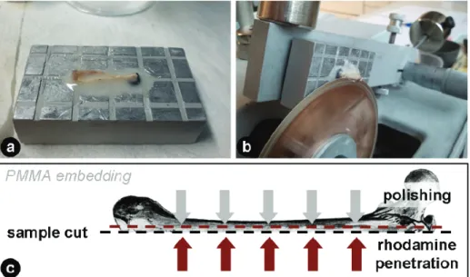
For rhodamine staining in combination with PMMA embedding, 0.002 % wt of rhodamine was dissolved in methyl metacrylate (MMA) and used as staining solution (3 times 1 day) during the dehydration series of the bone samples. Sub- sequently bone samples were embedded in covered plastic containers with PMMA solution containing 400 ml MMA, 100 ml nonylphenyl- polyethylene- glycol acetate (NPA) and 10 g dibenzoyl peroxide (BPO). During embedding samples were put to an oven at 42 °C for 12 hours, 48 °C for another 12 hours and for final hardening to 58 °C for 24 hours.

4.3.1.3 Scanning Electron Microscopy and Back-scattered Electron Microscopy

Dry bone samples were glued on an object holder with double sided tape and mounted on an aluminum stub. For examination a FEI-Quanta 600FEG electron microscope (FEICompany, Oregon, USA) was used in low vacuum mode (0.75 Torr) at a working distance of 10 mm. Images were taken with a solid state detector (SSD) at 15kV measuring the back-scattered-electron signal from the surface of the sample.

4.3.1.4 Cryo Scanning Electron Microscopy

Cryo SEM was performed in cooperation with Julia Mahamid at the Weizmann Institute of Science (WIS), Rehovot, Israel. To maintain transient mineral phases, samples had to be examined under the electron microscope using cryo conditions. This preparation protocol for bone samples is described elsewhere (Mahamid, Sharir et al. 2008). Fresh medullary bone pieces of approximately 500 x 500 x 200 microns were taken from the medullary cavity of the femur of a chicken directly after harvesting the bones. The samples were immediately im- mersed in 10% Dextran (Fluka – Sigma Aldrich GmbH, Germany), mounted between two metal discs (3 mm diameter, with 0.1 or 0.2 mm cavities) and cryo- immobilized in a high pressure freezing device HPM10 (Bal-Tec, Germany).

Subsequently samples were transferred to a Freeze Fracture device BAF 60 (Bal- Tec, Germany) and fractured at -140 °C, etched for 20 min and coated. Samples were observed in an Ultra 55 SEM (Zeiss, Germany) using a secondary electron in-lens detector and a backscattered electron in-lens detector (operating at 5 kV) in the frozen-hydrated state by use of a cryo-stage at a temperature of -120 °C.

(33)

4.3.1.5 Quantitative Back-scattered Electron Imaging

These measurements were performed in cooperation with Paul Roschger from the Ludwig Boltzmann Institute of Osteology in Vienna. More information about the experimental setup and calibration can be found elsewhere (Roschger, Fratzl et al. 1998). Bone samples containing a transversal fibrolamellar bone structure from the periosteal region down to the endosteal region were embedded in blocks of polymethylmethacrylate, polished and carbon coated by vacuum evaporation (SCD 004 Balzers, Liechtenstein). Examination was performed with a digital scanning electron microscope (DSM 962, Zeiss, Oberkochen, Germany) equipped with a four quadrant semiconductor back-scattered electron detector.

The microscope was set to an accelerating voltage of 20 kV and a working distance of 15 mm.

4.3.2 Small Angle X-ray Scattering Measurements

Small angle x-ray scattering is used to measure inhomogeneities of the nanos- tructure of a sample by elastic scattering of the x-ray beam. The signal contains amongst others information about the size and shape of macromolecules or pores.

In bone SAXS is used to study the dimension and the alignment of mineral particles which allows a better understanding of bone formation and remodeling.

Within this project bone samples were studied at two different synchrotron beamlines – the µSpot at BESSY II (Helmholtz-Zentrum Berlin für Materialien und Energie GmbH, Berlin, Germany) as well as the Nanofocus beamline ID13 at the European Synchrotron Radiation Facility (ESRF), Grenoble, France. The most relevant difference between these beamlines was the size of the x-ray beam and thus the maximum scanning resolution accessible. At BESSY a nominal beam size of ~ 15 µm could be obtained whereas at ID13 a beam size of ~ 500 nm could be used for scans. Here the experimental setup and measurement parameters at both beamlines are briefly described. Data correction and analysis of experiments with FIT2D and Autofit is similar and described subsequently.

4.3.2.1 Experimental Setup at BESSY

Ovine and murine bone samples with a thickness of approximately 30 µm were measured at the µSpot beamline with multi layer setup and a monochromatic x-

(34)

ray beam of 15keV. Sample to detector distance was set to ~ 300 mm for measurement with a 2D position-sensitive CCD-detector (MarMosaic 225, Mar USA Evanston, USA) with 3072 x 3072 pixels and a corresponding pixel size of 73.242 x 73.242 µm². To improve measurement time the detector binning was set to 2 x 2 (1536 x 1536 pixels, corresponding pixel size of 146.484 x 146.484 µm²) and the sample detector distance increased to ~ 400 mm to assure sufficient q- resolution. Bone samples were fixed with a lead tape and mounted on a sample holder screwed on an xyz translation stage which could be moved perpendicularly to the beam, allowing to measure the sample in scanning mode with a step size of 10 µm. Additionally an x-ray fluorescence (XRF) detector (ASAS-SDD, KETEK Germany) was used to measure calcium fluorescence signal simultaneously. For data correction, transmission intensity of each scanning point was measured with a diode before each area scan. The exposure time for the transmission measurements was set to 0.3 seconds. For measurement of the scattering pattern, exposure times were set accordingly to the binning factor, sample properties and the x-ray beam intensity between 4 and 30 seconds. A detailed description of the beamline can be found elsewhere (Paris, Li et al. 2007).

4.3.2.2 Experimental Setup at ESRF

At the Nanofocus beamline at ESRF ovine bone samples with a thickness of approximately 30µm were measured. A monochromatic x-ray beam with an energy of 14 keV was used. Scattering patterns were measured with an ESRF FReLoN detector with 2048 x 2048 pixels and a corresponding pixel size of 51.5 x 50.7 µm² (after flat field correction). To reduce measurement time detector binning was set to 4x4 (512 x 512 pixels, corresponding resolution of 205.9 x 202.8 µm²). The sample to detector distance was set to approximately 720 mm. Ovine bone samples were framed with a lead tape and screwed on a sample holder which was magnetically mounted to the sample stage. During the scan the stage was translated in yz direction, perpendicularly to the beam, with a step size of 1 µm. Simultaneously to the measurements of the scattering patterns, the calcium fluorescence signal was obtained with an XRF detector which was moved approximately 20 mm apart from the sample. Before each scan, transmission intensity of each scanning point was measured with a diode for later data correction.

The exposure time for the transmission measurements was set to 0.1 seconds. For

(35)

measurement of the scattering patterns, exposure times were set between 0.1 and 1 second.

4.3.2.3 Data Correction

Using Fit2d (Hammersley, Svensson et al. 1996) the sample to detector distance and the exact beam center position was determined from the diffraction patterns of hydroxyapatite (HAP) standard powder measured before and after each scan.

In order to correctly correlate background measurements with the measured scattering patterns a correction factor was determined:

⎟⎟

⎠

⎞

⎜⎜

⎝

⋅⎛

⎟⎟

⎠

⎞

⎜⎜

⎝

=⎛

∗

=

mar EB

mar sample diode

EB diode sample

Monitor Monitor I

t I t t

, , ,

, 2

1

with t1 as the correction of the transmission intensity which is the ratio of the Intensity at the Sample (Isample) and the empty beam intensity (IEB); and t2 as the correction of the decreasing beam intensity during scanning – measured with a beam monitor – due to the decrease of the ring current. For t1 the decrease of the ring current during the transmission scan was neglected since transmission scans were very short. Additionally the calcium fluorescence signal was corrected with t2 since a reduction in beam intensity leads to a lower fluorescence signal. The intensity correction of the scattering patterns was calculated by Autofit as followed:

mar EB mar sample

corrected I

t

I = I ^, − _,

4.3.2.4 Data Analysis

The data were analyzed using Autofit (custom made analysis software, C. Li, MPI of Colloids and Interfaces, Potsdam, Germany). For calculation of the T- parameter the following equations were used:

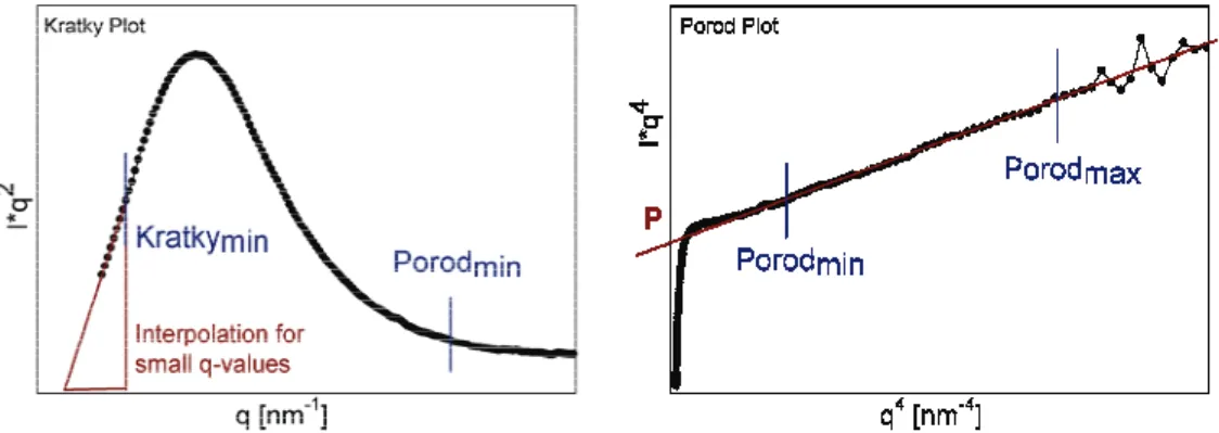
P T = ⋅ I

π 4

(36)

with Ī as the integration of the Kratky plot (Figure 7) and P the Porod constant as the intercept of the Porod fit with the ordinate (Figure 7). Ī was further calculated with

∫ ∫ ∫

∫

^∞

∞ = + +

=

min , ,

0 , ,min

2 min

, ,

min . ,

2 2

0

2 ( ) ( ) ( ) ( )

Kratky q

Porod q Porod

q

Kratky q

dq q I q dq

q I q dq

q I q

I r r r r

which further simplifies to

min , min

, ,

min , ,

2 min

. min

, ( )

2 1

Porod Porod

q

Kratky q Kratky Kratky

q dq P q I q q

I

I = ⋅ +

∫

^r +

as for biphasic systems the following equation is valid

) 4

( q

q P

I ⎯^q⎯ →^→⎯^∞

Fitting parameters for the Porod plot were set accordingly to different bone samples, since different bone types feature different mineral particle sizes. For ovine bone the Porod fit was set from Porodmin = 1.5 to Porodmax = 2.8 nm^-1. The Porod fit parameters for murine bone were set from 1.8 to 3.1 nm^-1. The fit parameter Kratkymin, from which the run of the Kratky plot is interpolated for small q- values (due to insufficient q-resolution), was set constantly to 0.3 nm^-1.

For the calculation of the Rho-parameter the scattering intensity integrated over q as a function of the azimuthal angle χ is analyzed. The distribution of the integrated intensity over χ shows two peaks (Figure 8) which are fitted with two Gaussian functions. The peak position of each Gaussian indicates the alignment of the mineral particles. To calculate the Rho-parameter, which describes the ratio of aligned particles to the total amount of particles in the illuminated area, the following equation is used:

0 2 1

2 1

A A A

A A Mineral

Mineral Rho

unaligned aligned

aligned

+ +

= +

=

+

(37)

with A1 and A2 as the area under both Gaussians respectively, interpreted as the amount of aligned particles and A0 as the area under the baseline of both Gaus- sians which can be interpreted as the fraction of unaligned particles.

Figure 7: Kratky and Porod plot from radially integrated SAXS patterns. The T-parameter calculation needs the user input of following parameters: Kratkymin Porodmin, Porodmax

Figure 8: Azimuthal plot of the scattering intensity showing two peaks which are 180° sepa- rated. A1+A2 describes the fraction of aligned particles, A0 the fraction of randomly aligned particles.

(38)

4.3.3 Quantitative Synchrotron Micro Computer Tomography

Medullary bone samples from chicken at 4 different time points (0, 6, 12, 18 hours after lay, 2 samples each) were examined using a 23 keV x-ray beam at the BAMline at BESSY II Helmholtz-Zentrum Berlin für Materialien und Energie GmbH, Berlin, Germany) to determine bone properties such as the degree of mineralization and trabecular architectures. For measurements, 1 cm long intact sections from the midshaft of the femur were embedded in blocks of polymethylmethacrylate as fixation. Samples were prepared completed anhydrously (see chapter 5), stacked onto each other and mounted to a rotation stage. For quantitative measurement of the bone mineral density, the sample to detector distance was set to 15 mm to prevent the influence of straylight and the measurement of coherence effects. For phase enhanced imaging, which improves the visualization of macroscopic edges of the bone architecture, the sample to detector distance was set to 40 mm. For each scan a total number of 1200 projections was measured with different resolutions ranging from 0.876 up to 4.34 µm. A more detailed description of the beamline setup can be found elsewhere (Rack, Zabler et al. 2008). The projection images were normalized and reconstructed using PyHST (Mirone, Wilcke et al. 2009)

4.3.4 Ptychography at the Swiss Light Source (SLS)

The experiments were performed in cooperation with Martin Dierolf from the Technical University Munich at the cSAXS beamline at the Swiss Light Source (SLS) which is part of the Paul Scherrer Institute (PSI), Villigen, Switzerland. In this experiment ovine bone samples, which where chemically treated with So- dium chloride solution and subsequently cut to small 2 mm long beams with a cross section of approximately 50 x 50 microns were scanned. As a standard measurement single spheres of HA powder with a diameter of approximately 30 µm were scanned. The cSAXS beamline is optimized for coherent SAXS appli- cations. A monochromatic x-ray beam with an energy of 6.2 keV, running through a small aperture, with a diameter of 2 to 3 µm was used. The detector (Pilatus 2M) was located at a distance of 7.19 m behind the sample in order to fulfill the required conditions for coherent diffractive imaging. The small beams of treated ovine bone were glued at the tip of a syringe and mounted close behind

(39)

the beam-defining pinhole to a three-axis piezo scanning stack located on top of an air bearing rotation stage. For each tomographic scan, 361 projections with a step size of 0.5° were taken. For each projection a ptychographic raster scan contains approximately 450 single scan points which overlap at adjacent positions.

Due to the overlap an improved convergence behavior of the image reconstruc- tion is obtained. With an exposure time of 0.1 seconds with an additional scanning overhead of another 0.1 seconds, scanning a field of view of approximately 65 x 20 µm² took about 12 hours. A more detailed description of ptychography measurements and data analysis as well as reconstructions can be found elsewhere (Dierolf, Menzel et al. 2010).

4.3.5 Infrared Spectroscopy

Infrared (IR) spectroscopy was performed together with Yotam Asscher from the Weizmann Institute of Science (WIS), Rehovot, Israel. More information on the influence of different sample preparation procedures can be found elsewhere (Asscher, Weiner et al. 2011). Freshly dissected pieces of medullary bone were washed with acetone to remove fatty tissue components. Samples were subsequently crushed in an agate mortar with sodium hypochlorite solution (6%) added for 5 minutes at room temperature. The suspension was then transferred into Eppendorf tubes and centrifuged at 14,000 rpm for 3 min in an Eppendorf 5417C micro centrifuge to remove the supernatant. The pellet was washed three times with double distilled water saturated with calcium and phosphate and twice with 100% ethanol. The pellet was resuspended in ethanol and sonicated (Ultra- sonicprocessor W-380; Heat Systems Ultrasonics). This procedure is known to not alter transient mineral phases (Mahamid, Sharir et al. 2008). The freshly sus- pended medullary bone mineral particles were subsequently exposed to a heat lamp in order to remove the remaining ethanol. The residual bone mineral was lightly crushed in an agate mortar, mixed with potassium bromide (KBr) and a 7- mm pellet was prepared. The IR-spectra were measured with a Nicolet 380 FTIR spectrometer. The splitting factor of the phosphate υ4 peak describing the crystal- linity of the bone material was calculated following Weiner and Bar-Yosef (Weiner and Bar-Yosef 1990).

(40)

4.4 Data Treatment and Visualization

All images obtained from microscopy-techniques as well as reconstructions from micro CT were edited and processed in ImageJ (National Institutes of Health, USA). Three-dimensional volumes were visualized using Drishti – Volume Ex- ploration and Visualization Tool (VizLab, The Australian National University).

Plotting of Data was done in SigmaPlot (Systat Software, Inc., USA) and Origin (OriginLab Corporation, USA).

(41)

5 Development of Experimental Procedures

The position resolved correlation of bone material properties with the osteocyte network geometries requires a variety of complementary experimental methods which all have to be performed at the same sample area. Thus bone preparation- and experimental procedures become a crucial issue and all have to be mutually accommodated. This chapter describes experimental- and sample preparation procedures which were developed during this project. These procedures such as the three-dimensional visualization of osteocyte networks, anhydrous sample preparation to not alter mineral properties as well as special labeling of scanning areas for confocal microscopy and scanning SAXS are essential for addressing the question whether osteocytes can influence their surrounding bone material.

5.1 Visualization of Osteocyte Networks

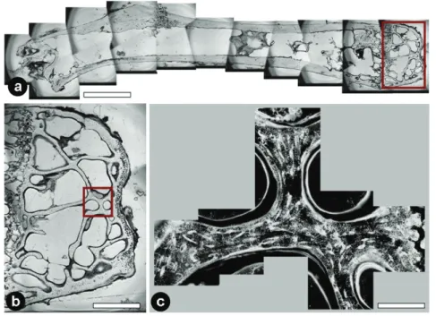
Visualizing osteocyte networks in undecalcified bone tissue is yet a great chal- lenge (Schneider, Meier et al. 2010) since resolving of canaliculi structures featuring diameters smaller then 100 nm involves scanning techniques with high spatial resolution. In principle two main approaches for visualization of the network structures are possible: Firstly micro- or even nano-computed tomography allows the assessment of volumes of various shapes (optimal signals with cylin- drical shapes). These can be performed either at lab sources or at the synchrotron. The final resolution of the scan is hereby defined by the technical setup and – even more important – by the dimension of the exposed sample volume. This leads to the fact that an increase in scanning resolution involves more sophisticated sample preparation since scanned volumes need to be smaller. As an example, for µCT scans at the BAMline at BESSY with a resolution of 3.5 µm cylin- drical objects of a maximal height of 14 mm and maximal diameter of 9.3 mm was measured. For a maximal resolution of 0.22 µm sample dimensions are already limited to a maximal height of 0.9 mm and a diameter of 0.6 mm. How- ever, to visualize canaliculi connecting the cells, a final pixel resolution smaller then 100 nm is required (Figure 9).

(42)

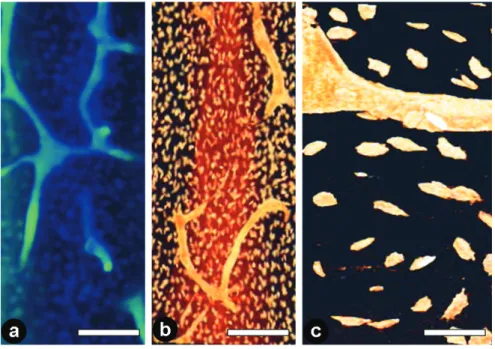
Figure 9: Visualization of osteocyte networks with different micro CT setups: (a) Skyscan 1072 with a pixel resolution of 10µm, (b) BAMline at BESSY II with a pixel resolution of 440 nm and (c) Skyscan NanoCT 2011 with a pixel resolution of 150 nm. Scale bars: (a), (b) 200µm, (c) 50 µm. None of these setups is capable of resolving canalicular structures in bone.

Secondly Confocal Laser Scanning Microscopy (CLSM) combined with fluorescent staining was applied on thin bone sections with a maximum thickness of 200 µm. The fluorescent dye gets excited by a laser with a suitable energy. The position of the emitted light was measured in a three-dimensional mode since the laser is accurately focused over the different z-levels of the sample (minimal step size of 0.2 µm) leading to a three-dimensional data output comparable to reconstructed data of a CT-scan. A substantial advantage of CLSM is the required sample dimension. These are fairly similar to those needed for different microscopical techniques as well as x-ray scattering measurements. Thus, a correlation of data from complementary experimental techniques from identical sample areas becomes feasible. Here rhodamine was used as staining solution diffusing through the blood vessels and osteocyte network binding to the cell membranes and mineral edges. Due to the high quantum efficiency of nearly one, high penetration depths of the measurement up to 50 µm are achievable (Figure 10). Even though a maximum pixel resolution of only approximately 0.2 µm is possible,