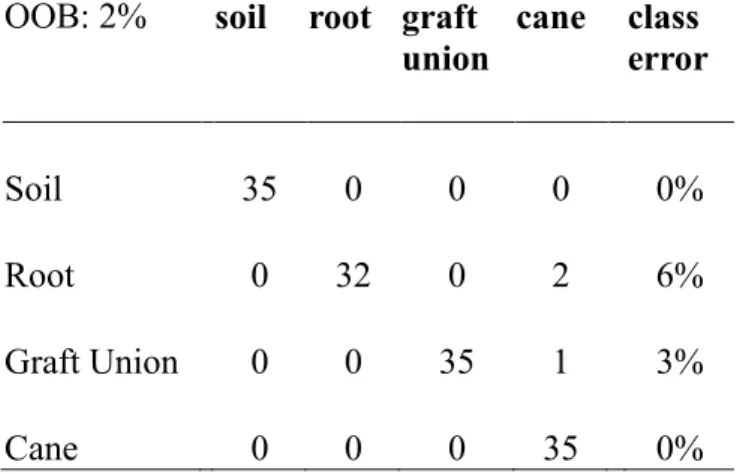
TABLE S1 Classification of the grapevine-associated microbiota attained by performing a

(1)

(2)

TABLE S1 Classification of the grapevine-associated microbiota attained by performing a

supervised learning analysis according to the factor sampling site (Random Forest). The predicted sample site classifications (soil, root, graft union, cane; horizontal) were compared to the known classifications of the sample sites (vertical). The percentage of wrongly classified samples within one sample site is called class error while the percentage of wrongly classified samples of all classified samples is termed the out-of-bag error (OOB: 2%).

OOB: 2% soil root graft

union cane class error

Soil 35 0 0 0 0%

Root 0 32 0 2 6%

Graft Union 0 0 35 1 3%

Cane 0 0 0 35 0%

(3)

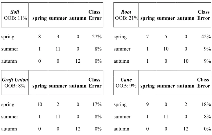
TABLE S2 Grapevine-associated microbiota were used to perform a supervised learning analysis (Random Forest) according to the factor season. Predicted classifications of the samples into spring, summer and autumn (horizontal) were compared to the known classifications in spring summer and autumn (vertical). The percentage of wrongly classified samples within one season is called class error while the percentage of wrongly classified samples within one sample site (soil, root, graft union, cane) is called out-of-bag error (OOB).

Soil Class Root Class

OOB: 11% spring summer autumn Error OOB: 21% spring summer autumn Error

spring 8 3 0 27% spring 7 5 0 42%

summer 1 11 0 8% summer 1 10 0 9%

autumn 0 0 12 0% autumn 1 0 10 9%

Graft Union Class Cane Class OOB: 8% spring summer autumn Error OOB: 9% spring summer autumn Error

spring 10 2 0 17% spring 9 0 2 18%

summer 1 11 0 8% summer 1 11 0 8%

autumn 0 0 12 0% autumn 0 0 12 0%

(4)

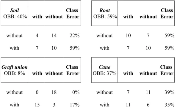
TABLE S3 Classification of the grapevine-associated microbiota according to the factor crown gall from performing a supervised learning analysis (Random Forest). The predicted

classification of the sample sites from grapevines with and without a crown gall (horizontal) are compared to the known sample site classifications of grapevines with and without a crown gall (vertical). The percentage of wrongly classified samples of grapevines with or without a crown gall is called class error while the percentage of wrongly classified samples within one sampling site (soil, root, graft union, cane) is termed an out-of-bag error (OOB).

Soil Class Root Class OBB: 40% with without Error OBB: 59% with without Error

without 4 14 22% without 10 7 59%

with 7 10 59% with 7 10 59%

Graft union Class Cane Class OBB: 8% with without Error OBB: 37% with without Error

without 0 18 0% without 7 11 39%

with 15 3 17% with 11 6 35%

(5)

factor comparision (A / B) A B logFC logCP p-value FDR class order genus species OTU with / without 1191 8 7.0 15.3 3.19E-13 4.71E-10 α-Proteobacteria Rhizobiales Agrobacterium vitis OTU_0003 with / without 4159 94 5.4 17.1 7.06E-07 2.98E-04 -Proteobacteria Pseudomonadales Pseudomonas NA OTU_0005

with / without 1872 10 7.4 15.9 4.03E-13 5.10E-10 -Proteobacteria Enterobacteriales NA NA OTU_0008

with / without 121 8 3.7 12.1 1.65E-09 1.46E-06 α-Proteobacteria Sphingomonadales Novosphingobium NA OTU_0022

with / without 985 1 9.1 15.0 3.27E-37 2.89E-33 -Proteobacteria Enterobacteriales Sodalis NA OTU_0043

with / without 56 5 3.2 11.1 1.41E-06 5.66E-04 Actinobacteria Actinomycetales Mycobacterium NA OTU_0065

with / without 92 0 6.4 11.7 1.87E-14 3.31E-11 -Proteobacteria Xanthomonadales Xanthomonas NA OTU_0076

with / without 107 2 5.1 11.9 3.34E-08 2.47E-05 α-Proteobacteria Rhizobiales Bosea genosp. OTU_0180

with / without 26 0 4.4 10.1 5.79E-07 2.70E-04 -Proteobacteria Xanthomonadales NA NA OTU_0188

with / without 45 0 5.4 10.7 8.63E-17 1.91E-13 Flavobacteriia Flavobacteriales Flavobacterium NA OTU_0248 with / without 24 0 4.3 10.0 3.14E-07 1.82E-04 Sphingobacteriia Sphingobacteriales Pedobacter NA OTU_0271

with / without 24 0 4.5 10.0 6.74E-13 7.46E-10 α-Proteobacteria Rhodospirillales NA NA OTU_0288

with / without 22 0 4.0 9.9 2.87E-09 2.31E-06 α-Proteobacteria Sphingomonadales Sphingomonas NA OTU_0421

with / without 23 1 3.7 9.9 4.72E-08 3.22E-05 α-Proteobacteria Rhizobiales NA NA OTU_1129

with / without 1 244 -7.2 13.0 4.03E-07 2.10E-04 -Proteobacteria Pseudomonadales Pseudomonas NA OTU_2368

with / without 875 1 9.1 14.8 9.27E-30 4.11E-26 -Proteobacteria NA NA NA OTU_3436

with / without 523 0 8.7 14.1 1.78E-18 5.26E-15 -Proteobacteria Enterobacteriales Erwinia NA OTU_7832

with / without 50 0 5.3 10.9 7.65E-08 4.84E-05 Actinobacteria Actinomycetales NA NA OTU_8550

with / without 120 11 3.3 12.6 2.71E-07 4.80E-04 α-Proteobacteria Rhizobiales Agrobacterium vitis OTU_0003 with / without 38 1380 -5.1 16.0 9.48E-08 4.20E-04 -Proteobacteria Pseudomonadales Pseudomonas NA OTU_0005 with / without 1 139 -6.0 12.7 1.13E-09 1.00E-05 Actinobacteria Actinomycetales Curtobacterium NA OTU_0011 with / without 4 171 -5.1 13.0 1.58E-07 4.27E-04 α-Proteobacteria Sphingomonadales Sphingomonas NA OTU_0052

with / without 37 1 4.4 11.0 1.93E-07 4.27E-04 -Proteobacteria NA NA NA OTU_3436

with / without 1230 1 9 16 9.51E-31 2.10E-27 α-Proteobacteria Rhizobiales Agrobacterium vitis OTU_0003

with / without 1855 2 9 16 8.13E-22 1.44E-18 -Proteobacteria Pseudomonadales Pseudomonas NA OTU_0005

with / without 345 1 8 14 2.18E-10 1.76E-07 α-Proteobacteria Rhizobiales Methylobacterium NA OTU_0006

with / without 509 11 5 14 1.86E-09 1.18E-06 -Proteobacteria Burkholderiales NA NA OTU_0007

with / without 3315 8 9 17 1.17E-13 1.15E-10 -Proteobacteria Enterobacteriales NA NA OTU_0008

with / without 87 8 3 12 6.55E-07 3.05E-04 α-Proteobacteria Sphingomonadales Sphingomonas NA OTU_0013

with / without 168 1 6 13 4.01E-15 4.43E-12 α-Proteobacteria Sphingomonadales Novosphingobium NA OTU_0022

with / without 252 15 4 13 1.06E-08 6.26E-06 α-Proteobacteria Rhizobiales Agrobacterium NA OTU_0032

with / without 352 0 8 14 1.19E-61 1.05E-57 -Proteobacteria Enterobacteriales Sodalis NA OTU_0043

with / without 61 1 5 11 1.60E-47 7.10E-44 Actinobacteria Actinomycetales Mycobacterium NA OTU_0065

with / without 103 0 6 12 2.06E-15 2.61E-12 -Proteobacteria Xanthomonadales Xanthomonas NA OTU_0076

with / without 87 1 5 12 1.38E-06 6.12E-04 α-Proteobacteria Rhizobiales Methylopila NA OTU_0121

with / without 67 1 5 11 1.38E-10 1.22E-07 Cytophagia Cytophagales Dyadobacter NA OTU_0144

with / without 26 1 3 10 1.84E-06 7.74E-04 Actinobacteria Actinomycetales Salinibacterium NA OTU_0210

with / without 25 1 4 10 1.21E-09 8.92E-07 α-Proteobacteria Sphingomonadales Sphingomonas NA OTU_0421

with / without 26 1 4 10 6.62E-16 9.77E-13 -Proteobacteria Burkholderiales NA NA OTU_3153

with / without 611 1 8 15 4.64E-38 1.37E-34 -Proteobacteria NA NA NA OTU_3436

bacterial classification

spr ing

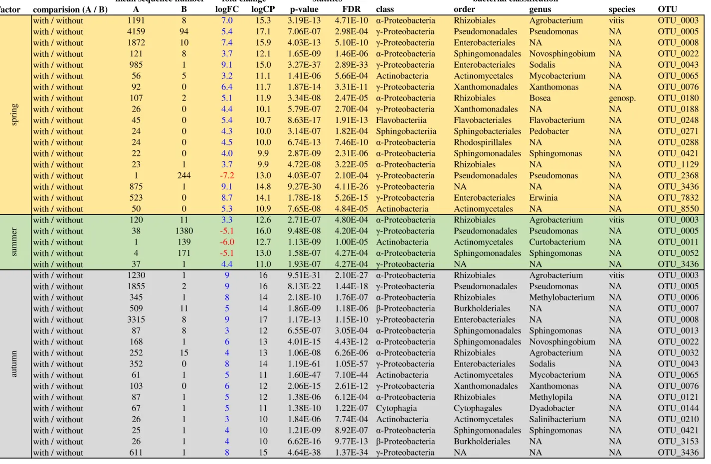
TABLE S4 Operational taxonomic units (OTUs) with significant differences (FDR < 0.001) in the mean number of 16S rRNA gene amplicon sequences. Differences between graft unions with 'A' and without 'B' crown gall disease in spring, summer, and autumn. Fold changes are given as log2FC and log2CPM (average log2 counts per million). Statistics analysis was performed using a two- sided test for calculation of the p-values. The false discovery rate (FDR) gives an adjusted p-value for multiple testing according to Benjamin-Hochberg.

summer autumn

mean sequence number fold change statitics

(6)

# R script for statistical analysis of microbiota in one vineyard in Franconia and in vitro grown grapevine plantlets

# datasource: SRA:EBI database (http://www.ebi.ac.uk/ena), project:

RJEB12040

# Title: Crown galls of grapevine (Vitis vinifera) host distinct microbiota; Authors: Hanna Faist, Alexander Keller, Ute Henschtel Humeida, Rosalia Deeken; Journal: AEM

#

#loading required packages library(phyloseq)

library(ggplot2)

library(vegan) # version 2.2-1 library(edgeR)

library(randomForest)#4.6-10 library(plyr)

######

#veganotu from

https://rdp.cme.msu.edu/tutorials/stats/using_rdp_output_with_phyloseq.ht ml, 2015-12-14, John Quensen and Qiong Wang

veganotu <- function(physeq) { OTU <- otu_table(physeq) if (taxa_are_rows(OTU)) { OTU <- t(OTU)

}

OTU <- as(OTU, "matrix") return(OTU)

}

####

# Phyloseq to EdgeR from http://joey711.github.io/phyloseq- extensions/edgeR.html, 2015-12-14

#########################################################################

#######

#' Convert phyloseq OTU count data into DGEList for edgeR package

#'

#' Further details.

#'

#' @param physeq (Required). A \code{\link{phyloseq-class}} or

#' an \code{\link{otu_table-class}} object.

#' The latter is only appropriate if \code{group} argument is also a

#' vector or factor with length equal to \code{nsamples(physeq)}.

#'

#' @param group (Required). A character vector or factor giving the experimental

#' group/condition for each sample/library. Alternatively, you may provide

(7)

#' the name of a sample variable. This name should be among the output of

#' \code{sample_variables(physeq)}, in which case

#' \code{get_variable(physeq, group)} would return either a character vector or factor.

#' This is passed on to \code{\link[edgeR]{DGEList}},

#' and you may find further details or examples in its documentation.

#'

#' @param method (Optional). The label of the edgeR-implemented normalization to use.

#' See \code{\link[edgeR]{calcNormFactors}} for supported options and details.

#' The default option is \code{"RLE"}, which is a scaling factor method

#' proposed by Anders and Huber (2010).

#' At time of writing, the \link[edgeR]{edgeR} package supported

#' the following options to the \code{method} argument:

#'

#' \code{c("TMM", "RLE", "upperquartile", "none")}.

#'

#' @param ... Additional arguments passed on to

\code{\link[edgeR]{DGEList}}

#'

#' @examples

#'

phyloseq_to_edgeR = function(physeq, group, method="RLE", ...){

require("edgeR") require("phyloseq") # Enforce orientation.

if( !taxa_are_rows(physeq) ){ physeq <- t(physeq) } x = as(otu_table(physeq), "matrix")

# Add one to protect against overflow, log(0) issues.

x = x + 1

# Check `group` argument

if( identical(all.equal(length(group), 1), TRUE) & nsamples(physeq) > 1 ){

# Assume that group was a sample variable name (must be categorical) group = get_variable(physeq, group)

}

# Define gene annotations (`genes`) as tax_table taxonomy = tax_table(physeq, errorIfNULL=FALSE) if( !is.null(taxonomy) ){

taxonomy = data.frame(as(taxonomy, "matrix")) }

# Now turn into a DGEList

y = DGEList(counts=x, group=group, genes=taxonomy, remove.zeros = TRUE, ...)

# Calculate the normalization factors z = calcNormFactors(y, method=method)

# Check for division by zero inside `calcNormFactors`

if( !all(is.finite(z$samples$norm.factors)) ){

stop("Something wrong with edgeR::calcNormFactors on this data, non-finite $norm.factors, consider changing `method` argument") }

# Estimate dispersions

return(estimateTagwiseDisp(estimateCommonDisp(z))) }

#########################################################################

#######

(8)

#funktion to make multiple plots from http://www.cookbook-

r.com/Graphs/Multiple_graphs_on_one_page_%28ggplot2%29/, 2015-12-15

################################################

# Multiple plot function

#

# ggplot objects can be passed in ..., or to plotlist (as a list of ggplot objects)

# - cols: Number of columns in layout

# - layout: A matrix specifying the layout. If present, 'cols' is ignored.

#

# If the layout is something like matrix(c(1,2,3,3), nrow=2, byrow=TRUE),

# then plot 1 will go in the upper left, 2 will go in the upper right, and

# 3 will go all the way across the bottom.

#

multiplot <- function(..., plotlist=NULL, file, cols=1, layout=NULL) { require(grid)

# Make a list from the ... arguments and plotlist plots <- c(list(...), plotlist)

numPlots = length(plots)

# If layout is NULL, then use 'cols' to determine layout if (is.null(layout)) {

# Make the panel

# ncol: Number of columns of plots

# nrow: Number of rows needed, calculated from # of cols layout <- matrix(seq(1, cols * ceiling(numPlots/cols)), ncol = cols, nrow = ceiling(numPlots/cols)) }

if (numPlots==1) { print(plots[[1]])

} else {

# Set up the page grid.newpage()

pushViewport(viewport(layout = grid.layout(nrow(layout), ncol(layout))))

# Make each plot, in the correct location for (i in 1:numPlots) {

# Get the i,j matrix positions of the regions that contain this subplot

matchidx <- as.data.frame(which(layout == i, arr.ind = TRUE))

print(plots[[i]], vp = viewport(layout.pos.row = matchidx$row, layout.pos.col = matchidx$col)) }

} }

#########################################################################

###########

##set local directions

(9)

treefile="<PATH-TO-DATA>\\otus.tre"

otufile="<PATH-TO-DATA>\\otus.ncmt.biom"

mapfile="<PATH-TO-DATA>\\mapfile-vers1.txt"

#otufile2 was not filtered for plastids and mitochondria otufile2="<PATH-TO-DATA>\\otus.tax.biom"

##import data

otu= import_biom(otufile, parseFunction= parse_taxonomy_greengenes) map = import_qiime_sample_data(mapfile)

tree=read_tree(treefile)

datensatz=merge_phyloseq(otu, map, tree)

#without filtering for plastids and chloroplasts

otu2= import_biom(otufile2, parseFunction= parse_taxonomy_greengenes) datensatz2=merge_phyloseq(otu2, map, tree)

## generate a sub dataset with in vitro grown grapevine plantlets

BlankIVS= subset_samples(datensatz,(sample_data(datensatz))$Study ==

"seasons-invitro" )

Invitro1= subset_samples(datensatz,(sample_data(datensatz))$Study ==

"invitro" )

Invitro=merge_phyloseq(BlankIVS, Invitro1)

Invitro= subset_samples(Invitro,(sample_data(Invitro))$grapevariety !=

"silvaner" ) #silvaner was not used for the study as A.vitis sequences were found in this variety of in vitro grapevine plantlets

GV=subset_samples(Invitro,(sample_data(Invitro))$Crown_gall == "GV3101" ) S7=subset_samples(Invitro,(sample_data(Invitro))$Crown_gall == "A.vitis"

)

no=subset_samples(Invitro,(sample_data(Invitro))$Crown_gall == "no" ) Invitro_18=merge_phyloseq(GV,S7,no)

## generate sub datasets with grapevine and soil samples from the vineyard

Seasons1= subset_samples(datensatz,(sample_data(datensatz))$Study ==

"seasons")

Seasons1= subset_samples(Seasons1, (sample_data(Seasons1))$Season !=

"graftgall") # exclude grapevine samples which are not a part of the publication as they are not from the same vineyard

BlankIVS= subset_samples(datensatz,(sample_data(datensatz))$Study ==

"seasons-invitro" )

Seasonsdatabl=merge_phyloseq(Seasons1, BlankIVS) Seasonsdata_c1=subset_samples(Seasonsdatabl,

(sample_data(Seasonsdatabl))$Crown_gall != "blank") #exclude negative controls (c1) without any material

Seasonsdata_c2=subset_samples(Seasonsdata_c1,

sample_data(Seasonsdata_c1)$Kit == "MP") # exclude soil samples done with another dna-extraction kit (c2)

Seasonsdata_144= subset_samples(Seasonsdata_c2, X.SampleID!="HF055") #One DNA-extraction was analyzed on two different sequencing chips, the second sample was excluded - now 144 samples as decribed in FIG_1C remain

(10)

# remove outliers

Seasonsdata = subset_samples(Seasonsdata_144, X.SampleID!="HF009") Seasonsdata = subset_samples(Seasonsdata, X.SampleID!="HF060") Seasonsdata = subset_samples(Seasonsdata, X.SampleID!="HF096") Seasonsdata = subset_samples(Seasonsdata, X.SampleID!="HF140")

# separate data according to sources

Trunkdata=subset_samples(Seasonsdata, (sample_data(Seasonsdata))$Source

== "trunk")

Canedata=subset_samples(Seasonsdata, (sample_data(Seasonsdata))$Source ==

"cane")

Rootdata=subset_samples(Seasonsdata, (sample_data(Seasonsdata))$Source ==

"root")

Soildata=subset_samples(Seasonsdata, (sample_data(Seasonsdata))$Source ==

"soil")

# restrict to graft union samples and separate them according to crown gall disease and seasons

# GU= graftunion, CG=crown_gall, NGGU=Non-galled graft union, Au=autumn, Sp=apring, Su=summer

GU_data=Trunkdata

CG_data=subset_samples(GU_data, (sample_data(GU_data))$Crown_gall ==

"present")

NGGU_data=subset_samples(GU_data, (sample_data(GU_data))$Crown_gall ==

"absent")

Au_data=subset_samples(GU_data, (sample_data(GU_data))$Seasons ==

"autumn")

Sp_data=subset_samples(GU_data, (sample_data(GU_data))$Seasons ==

"spring")

Su_data=subset_samples(GU_data, (sample_data(GU_data))$Seasons ==

"summer")

NGGU_Au_data=subset_samples(NGGU_data, (sample_data(NGGU_data))$Seasons

== "autumn")

NGGU_Sp_data=subset_samples(NGGU_data, (sample_data(NGGU_data))$Seasons

== "spring")

NGGU_Su_data=subset_samples(NGGU_data, (sample_data(NGGU_data))$Seasons

== "summer")

CG_Au_data=subset_samples(CG_data, (sample_data(CG_data))$Seasons ==

"autumn")

CG_Sp_data=subset_samples(CG_data, (sample_data(CG_data))$Seasons ==

"spring")

CG_Su_data=subset_samples(CG_data, (sample_data(CG_data))$Seasons ==

"summer")

CG_AuSp_data=merge_phyloseq(CG_Au_data, CG_Sp_data) CG_AuSu_data=merge_phyloseq(CG_Au_data, CG_Su_data) CG_SuSp_data=merge_phyloseq(CG_Su_data, CG_Sp_data)

NGGU_AuSp_data=merge_phyloseq(NGGU_Au_data, NGGU_Sp_data) NGGU_AuSu_data=merge_phyloseq(NGGU_Au_data, NGGU_Su_data) NGGU_SuSp_data=merge_phyloseq(NGGU_Su_data, NGGU_Sp_data)

(11)

#### Results in the order of the paper

## Comparison of the environmental grapevine datasets with and without filtering for plastids and mitochondria

#dataset with plastids and mitochondria

Seasons1_2= subset_samples(datensatz2,(sample_data(datensatz2))$Study ==

"seasons")

Seasons1_2= subset_samples(Seasons1_2, (sample_data(Seasons1_2))$Season

!= "graftgall") #exclude grapevine samples which are not a part of the publication as they are not from the same vineyard

BlankIVS_2= subset_samples(datensatz2,(sample_data(datensatz2))$Study ==

"seasons-invitro" )

Seasonsdatabl_2=merge_phyloseq(Seasons1_2, BlankIVS_2) Seasonsdata_c1_2=subset_samples(Seasonsdatabl_2,

(sample_data(Seasonsdatabl_2))$Crown_gall != "blank") #exclude negative controls (c1) without any material

Seasonsdata_c2_2=subset_samples(Seasonsdata_c1_2,

sample_data(Seasonsdata_c1_2)$Kit == "MP") #exclude soil samples done with another dna-extraction kit (c2)

Seasonsdata_144_2= subset_samples(Seasonsdata_c2_2, X.SampleID!="HF055")

#One DNA-extraction was analyzed on two different sequencing chips, the second sample was excluded - now 144 samples as decribed in FIG_1C remain

sum(otu_table(Seasonsdata_144_2)) #total sequences with plastids and mitochondria

sum(otu_table(Seasonsdata_144)) #total sequences without plastids and mitochondria

Seasonsdata_144_gr0= prune_taxa(taxa_sums(Seasonsdata_144)>0, Seasonsdata_144) #remove taxa with no sequences in this dataset

## FIG 2A: Non metric multidimensional scaling analysis using the Bray Curtis distance to show differences between microbiomes of grapevine and soil material

# calculate non metric multidimensional (NMDS) scaling NSe=ordinate(Seasonsdata, "NMDS", distance="bray")

# plot NMDS

NMDS_Source= plot_ordination(Seasonsdata, NSe, axes=c(1,2), color="Source") +geom_point(size =7)+ theme_classic()

NMDS_Source

# environmental fit for finding significant factors that influence the data

envfit(NSe, data.frame(sample_data(Seasonsdata)[,c(5,7,11)]))

#final layout was done with inkscape 0.91

(12)

## Analysing the influence of the factor season on the microbiome:

general linear model and anova

#extract scores of NMDS and link them to sample sheet

df=cbind(scores(NSe),data.frame(sample_data(Seasonsdata)[,c(6,5,7,11)]))

#calculate the general lineal model and show the summary results summary(glm(NMDS1~Source,data=df))

#test the significance of the model by anova anova(glm(NMDS1~Source,data=df), test="F")

## STAB 1: Random forest categorisation of all samples according to different sources

Seasonsdata_rel = transform_sample_counts(Seasonsdata, function(x) x/sum(x))

RFSource_rel= randomForest(x = veganotu(Seasonsdata_rel), y =

data.frame(sample_data(Seasonsdata_rel))$Source, ntree = 2000, mtry = sqrt(ntaxa(Seasonsdata_rel)), importance = T, do.trace = 100) RFSource_rel #print details

#the table layout was done in excel

## FIG 3A Richness of different sources

#Observed=Richness

SeasonsObserved.biodiv=plot_richness(Seasonsdata , x="Source", measures

= c("Observed"), title="Richness")

#plot biodiversity

SeasonsObserved.biodiv + geom_boxplot(alpha = 1)+ theme_classic()+

scale_x_discrete(limits=c("soil", "root", "trunk", "cane"))

#table with Observed values

SeasonsObserved.tab= cbind(estimate_richness(Seasonsdata, measures=c("Observed")), sample_data(Seasonsdata))

#mean and sd per source

ddply(SeasonsObserved.tab, .(Source), summarize, mean_value = mean(Observed)) # mean per source

ddply(SeasonsObserved.tab, .(Source), summarize, sd_value = sd(Observed))

# sd per source

#significance by wilcoxon

wilcox.test(Observed~Source, data=SeasonsObserved.tab, subset= Source

%in% c("soil", "root"))

%in% c("soil", "trunk"))

%in% c("soil", "cane"))

%in% c("cane", "root"))

(13)

%in% c("cane", "trunk"))

%in% c("root", "trunk"))

## Percentage of shared OTUs of different sample sources

#extract the rownames of those OTUs with at least one sequence

source.venn=rownames(otu_table(Seasonsdata))[rowSums(otu_table(Seasonsdat a))>0.01]

trunk.venn=rownames(otu_table(Trunkdata))[rowSums(otu_table(Trunkdata))>0 .01]

root.venn=rownames(otu_table(Rootdata))[rowSums(otu_table(Rootdata))>0.01 ]

soil.venn=rownames(otu_table(Soildata))[rowSums(otu_table(Soildata))>0.01 ]

cane.venn=rownames(otu_table(Canedata))[rowSums(otu_table(Canedata))>0.01 ]

#percentage of shared OTUs between all sources

venn_list.source= list(Soil=soil.venn, Root=root.venn, Trunk=trunk.venn, Cane=cane.venn)

p=(length(Reduce(intersect, venn_list.source))/length(source.venn))*100

#percentage of shared OTUs of one source with the soil (the OTUs of the non-soil source are=100%)

length(intersect(soil.venn,root.venn))/(length(root.venn)) length(intersect(cane.venn,soil.venn))/(length(cane.venn)) length(intersect(trunk.venn,soil.venn))/(length(trunk.venn))

#percentage of shared OTUS between two sources (unique OTUs in both sources are =100%)

length(intersect(soil.venn,root.venn))/(length(setdiff(soil.venn, root.venn))+ length(setdiff(root.venn,

soil.venn))+length(intersect(soil.venn,root.venn)))

length(intersect(trunk.venn,root.venn))/(length(setdiff(trunk.venn, root.venn))+length(setdiff(root.venn,

trunk.venn))+length(intersect(trunk.venn,root.venn)))

length(intersect(trunk.venn,cane.venn))/(length(setdiff(trunk.venn, cane.venn))+length(setdiff(cane.venn,

trunk.venn))+length(intersect(trunk.venn,cane.venn)))

length(intersect(cane.venn,soil.venn))/(length(setdiff(cane.venn, soil.venn))+length(setdiff(soil.venn,

cane.venn))+length(intersect(soil.venn,cane.venn)))

length(intersect(trunk.venn,soil.venn))/(length(setdiff(trunk.venn, soil.venn))+length(setdiff(soil.venn,

trunk.venn))+length(intersect(soil.venn,trunk.venn)))

length(intersect(cane.venn,root.venn))/(length(setdiff(cane.venn, root.venn))+length(setdiff(root.venn,

cane.venn))+length(intersect(root.venn,cane.venn)))

## FIG 3B alpha Diversity (Shannon) of different sources

#alpha diversity, Shannon Index

SeasonsShannon.biodiv=plot_richness(Seasonsdata , x="Source", measures = c("Shannon"), title="Shannon")

(14)

#plot biodiversity

SeasonsShannon.biodiv + geom_boxplot(alpha = 1)+ theme_classic()+

scale_x_discrete(limits=c("soil", "root", "trunk", "cane"))

#Table with Shannon values

SeasonsShannon.tab= cbind(estimate_richness(Seasonsdata, measures=c("Shannon")), sample_data(Seasonsdata))

#mean and sd per source

ddply(SeasonsShannon.tab, .(Source), summarize, mean_value = mean(Shannon)) # mean per source

ddply(SeasonsShannon.tab, .(Source), summarize, sd_value = sd(Shannon))

# sd per source

wilcox.test(Shannon~Source, data=SeasonsShannon.tab, subset= Source %in%

c("soil", "root"))

c("soil", "trunk"))

c("soil", "cane"))

c("cane", "root"))

c("root", "trunk"))

## FIG 3C: Relative phyla composition of microbiota of soil, root, graft union and canes

#merge all OTUs from the same phyla within one sample PhylSeasons=tax_glom(Seasonsdata, taxrank="Phylum")

#now we have instead of OTUs, different phyla-names

#merge all samples from the same source

PhylSeasons.M=merge_samples(PhylSeasons, "Source")

#calculate the relative abundance of each phylum in each sample type PhylSeasons.Mrel=transform_sample_counts(PhylSeasons.M, function(x) x/sum(x))

#merge all phyla with a relative abundance < 0.05 PhylSeasons.plot=merge_taxa(PhylSeasons.Mrel,

taxa_names(PhylSeasons.Mrel)[taxa_sums(PhylSeasons.Mrel)<0.05])

#create table

TablePhylSeasons=rbind(otu_table(PhylSeasons.plot),t(tax_table(PhylSeason s.plot)[,2]))

#save files

#write.table(TablePhylSeasons, "<PATH-TO-DATA>\\TablePhylSeasons")

# the layout of the barplot was done in excel

## FIG 3D: Relative genera composition of microbiota of soil, root, graft union and cane

(15)

#merge all OTUs from the same genus within one sample GenusSeasons=tax_glom(Seasonsdata, taxrank="Genus")

#now we have instead of OTUs, different Genera-names

#merge all samples from the same source

GenusSeasons.M=merge_samples(GenusSeasons, "Source")

#calculate the relative abundance of each genus in each sample type GenusSeasons.Mrel=transform_sample_counts(GenusSeasons.M, function(x) x/sum(x))

#merge all genera with a relative abundance < 0.05 GenusSeasons.plot=merge_taxa(GenusSeasons.Mrel,

taxa_names(GenusSeasons.Mrel)[taxa_sums(GenusSeasons.Mrel)<0.05])

#create table

TableGenusSeasons=rbind(otu_table(GenusSeasons.plot),t(tax_table(GenusSea sons.plot)[,6]))

#save files

#write.table(TableGenusSeasons, "<PATH-TO-DATA>\\TableGenusSeasons")

# the layout of the barplot was done in excel

## FIG 4: NMDS separated for each source and coloured according to crown gall disease and seasons

# calculate non metric multidimensional (NMDS) scaling plot NC=ordinate(Canedata, "NMDS", distance="bray")

NR=ordinate(Rootdata, "NMDS", distance="bray") NS=ordinate(Soildata, "NMDS", distance="bray") NT=ordinate(Trunkdata, "NMDS", distance= "bray")

# plot NMDS

FIG4BS= plot_ordination(Soildata, NS, axes=c(1,2), shape="Crown_gall", title="soil" ) +geom_point(size =4)+

theme_classic()+scale_shape_manual(values=c(17,15))+coord_cartesian(xlim

= c(-2, 2), ylim = c(-1.1,1))

FIG4BR= plot_ordination(Rootdata, NR, axes=c(1,2), shape="Crown_gall", title="root" ) +geom_point(size =4)+

= c(-2, 2), ylim = c(-1.1,1))

FIG4BT= plot_ordination(Trunkdata, NT, axes=c(1,2),shape="Crown_gall", title="graft union" ) +geom_point(size =4)+

= c(-2, 2), ylim = c(-1.1,1))

FIG4BC= plot_ordination(Canedata, NC, axes=c(1,2), shape="Crown_gall", title="cane" ) +geom_point(size =4)+

= c(-2, 2), ylim = c(-1.1,1))

FIG4AS= plot_ordination(Soildata, NS, axes=c(1,2), color="Seasons", title="soil" ) +geom_point(size =4)+

= c(-2, 2), ylim = c(-1.1,1))

FIG4AR= plot_ordination(Rootdata, NR, axes=c(1,2), color="Seasons", title="root" ) +geom_point(size =4)+

(16)

= c(-2, 2), ylim = c(-1.1,1))

FIG4AT= plot_ordination(Trunkdata, NT, axes=c(1,2),color="Seasons", title="graft union" ) +geom_point(size =4)+

= c(-2, 2), ylim = c(-1.1,1))

FIG4AC= plot_ordination(Canedata, NC, axes=c(1,2), color="Seasons", title="cane" ) +geom_point(size =4)+

= c(-2, 2), ylim = c(-1.1,1))

multiplot(FIG4BS,FIG4BT,FIG4BR,FIG4BC, cols=2) multiplot(FIG4AS,FIG4AT,FIG4AR,FIG4AC, cols=2)

# environmental fit for finding significant factors that influence the data

envfit(NT, data.frame(sample_data(Trunkdata)[,c(7,11)])) envfit(NC, data.frame(sample_data(Canedata)[,c(7,11)])) envfit(NR, data.frame(sample_data(Rootdata)[,c(7,11)])) envfit(NS, data.frame(sample_data(Soildata)[,c(7,11)]))

#the final layout of the multiplots was done in inkscape 0.91

##STAB 2: Random forest categorisation of graft union samples according to different seasons

Trunkdata_rel = transform_sample_counts(Trunkdata, function(x) x/sum(x)) Soildata_rel = transform_sample_counts(Soildata, function(x) x/sum(x)) Rootdata_rel = transform_sample_counts(Rootdata, function(x) x/sum(x)) Canedata_rel = transform_sample_counts(Canedata, function(x) x/sum(x))

RF_Tr_Se_rel= randomForest(x = veganotu(Trunkdata_rel), y =

data.frame(sample_data(Trunkdata_rel))$Seasons, ntree = 2000, mtry = sqrt(ntaxa(Trunkdata_rel)), importance = T, do.trace = 100) RF_So_Se_rel= randomForest(x = veganotu(Soildata_rel), y =

data.frame(sample_data(Soildata_rel))$Seasons, ntree = 2000, mtry = sqrt(ntaxa(Soildata_rel)), importance = T, do.trace = 100) RF_Ca_Se_rel= randomForest(x = veganotu(Canedata_rel), y =

data.frame(sample_data(Canedata_rel))$Seasons, ntree = 2000, mtry = sqrt(ntaxa(Canedata_rel)), importance = T, do.trace = 100) RF_Ro_Se_rel= randomForest(x = veganotu(Rootdata_rel), y =

data.frame(sample_data(Rootdata_rel))$Seasons, ntree = 2000, mtry = sqrt(ntaxa(Rootdata_rel)), importance = T, do.trace = 100)

RF_Ro_Se_rel RF_So_Se_rel RF_Ca_Se_rel

RF_Tr_Se_rel #print details

##STAB 3: Random forest categorisation of graft union samples according to the crown gall disease

Trunkdata_rel = transform_sample_counts(Trunkdata, function(x) x/sum(x)) Soildata_rel = transform_sample_counts(Soildata, function(x) x/sum(x))

(17)

Rootdata_rel = transform_sample_counts(Rootdata, function(x) x/sum(x)) Canedata_rel = transform_sample_counts(Canedata, function(x) x/sum(x))

RF_Tr_CG_rel= randomForest(x = veganotu(Trunkdata_rel), y =

data.frame(sample_data(Trunkdata_rel))$Crown_gall, ntree = 2000, mtry = sqrt(ntaxa(Trunkdata_rel)), importance = T, do.trace = 100)

RF_So_CG_rel= randomForest(x = veganotu(Soildata_rel), y =

data.frame(sample_data(Soildata_rel))$Crown_gall, ntree = 2000, mtry = sqrt(ntaxa(Soildata_rel)), importance = T, do.trace = 100)

RF_Ca_CG_rel= randomForest(x = veganotu(Canedata_rel), y =

data.frame(sample_data(Canedata_rel))$Crown_gall, ntree = 2000, mtry = sqrt(ntaxa(Canedata_rel)), importance = T, do.trace = 100)

RF_Ro_CG_rel= randomForest(x = veganotu(Rootdata_rel), y =

data.frame(sample_data(Rootdata_rel))$Crown_gall, ntree = 2000, mtry = sqrt(ntaxa(Rootdata_rel)), importance = T, do.trace = 100)

RF_Ro_CG_rel RF_Ca_CG_rel RF_So_CG_rel

RF_Tr_CG_rel #print details

##FIG 5A: Richness in graft union samples

#Observed=Richness

GU_Observed.biodiv=plot_richness(GU_data, color="Crown_gall" , x="Seasons", measures = "Observed", title="GU")

#plot biodiversity

GU_Observed.biodiv + geom_boxplot(alpha = 1)+ theme_classic()+

scale_x_discrete(limits=c("spring","summer","autumn"))+

scale_colour_manual(values = c("blue","red"))

#Table with Observed values

CG_Observed.tab= cbind(estimate_richness(CG_data, measures=c("Observed")), sample_data(CG_data))

NGGU_Observed.tab= cbind(estimate_richness(NGGU_data, measures=c("Observed")), sample_data(NGGU_data)) Au_Observed.tab= cbind(estimate_richness(Au_data, measures=c("Observed")), sample_data(Au_data)) Sp_Observed.tab= cbind(estimate_richness(Sp_data, measures=c("Observed")), sample_data(Sp_data)) Su_Observed.tab= cbind(estimate_richness(Su_data, measures=c("Observed")), sample_data(Su_data))

wilcox.test(Observed~Seasons, data=NGGU_Observed.tab, subset= Seasons

%in% c("summer", "autumn"))

wilcox.test(Observed~Seasons, data=NGGU_Observed.tab, subset= Seasons

%in% c("autumn", "spring"))

wilcox.test(Observed~Crown_gall, data=Au_Observed.tab) wilcox.test(Observed~Crown_gall, data=Su_Observed.tab) wilcox.test(Observed~Crown_gall, data=Sp_Observed.tab)

(18)

## FIG 5 B: Shannon index in galled and non-galled graft unions

#biodiversity

GU_Shannon.biodiv=plot_richness(GU_data, color="Crown_gall" , x="Seasons", measures = "Shannon", title="GU")

#plot biodiversity

GU_Shannon.biodiv + geom_boxplot(alpha = 1)+ theme_classic()+

scale_x_discrete(limits=c("spring","summer","autumn"))+

scale_colour_manual(values = c("blue","red"))

#Table with Shannon values

CG_Shannon.tab= cbind(estimate_richness(CG_data, measures=c("Shannon")), sample_data(CG_data))

NGGU_Shannon.tab= cbind(estimate_richness(NGGU_data, measures=c("Shannon")), sample_data(NGGU_data))

Au_Shannon.tab= cbind(estimate_richness(Au_data, measures=c("Shannon")), sample_data(Au_data))

Sp_Shannon.tab= cbind(estimate_richness(Sp_data, measures=c("Shannon")), sample_data(Sp_data))

Su_Shannon.tab= cbind(estimate_richness(Su_data, measures=c("Shannon")), sample_data(Su_data))

wilcox.test(Shannon~Seasons, data=CG_Shannon.tab, subset= Seasons %in%

c("summer", "autumn"))

wilcox.test(Shannon~Seasons, data=CG_Shannon.tab, subset= Seasons %in%

c("summer", "spring"))

wilcox.test(Shannon~Crown_gall, data=Au_Shannon.tab) wilcox.test(Shannon~Crown_gall, data=Su_Shannon.tab) wilcox.test(Shannon~Crown_gall, data=Sp_Shannon.tab)

## FIG 5 C, Three most abundant OTUs in the six different graft union typs (sp-cg, su-cg, au-cg, sp-nggu, su-nggu, au-nggu)

# merge all crown gall samples from the same season CG.M=merge_samples(CG_data, "Seasons")

NGGU.M=merge_samples(NGGU_data, "Seasons")

# rel

CG.Mrel=transform_sample_counts(CG.M, function(x) x/sum(x)) NGGU.Mrel=transform_sample_counts(NGGU.M, function(x) x/sum(x))

# order

CG_top_OTUs=t(otu_table(CG.Mrel))[order (t(otu_table(CG.Mrel))[,1], decreasing="TRUE"),]

NGGU_top_OTUs=t(otu_table(NGGU.Mrel))[order (t(otu_table(NGGU.Mrel))[,1], decreasing="TRUE"),]

#write table

#write.table(CG_top_OTUs, "<PATH-TO-DATA>\\CG-top-OTUs-percent")

#write.table(NGGU_top_OTUs, "<PATH-TO-DATA>\\NGGU-top-OTUs-percent")

#barplots were done in excel

(19)

## STAB 4: Different abundant OTUs in spring crown galls compared to spring non-galled graft unions. The analysis was repeated for summer and autumn

#convert phyloseq format to EdgeR format

A.EdgeRTrunk= phyloseq_to_edgeR(Au_data, group="Crown_gall") Sp.EdgeRTrunk= phyloseq_to_edgeR(Sp_data, group="Crown_gall") Su.EdgeRTrunk= phyloseq_to_edgeR(Su_data, group="Crown_gall")

# Perform binary test: logFC,logCMP and p-value of the comparison of the two groups

A.et = exactTest(A.EdgeRTrunk) Sp.et = exactTest(Sp.EdgeRTrunk) Su.et = exactTest(Su.EdgeRTrunk)

#create table with taxonomic rank, logFC, logCPM, P-value and FDR, sorted by p-value

A.tt = topTags(A.et, n=nrow(A.EdgeRTrunk$table), adjust.method="BH", sort.by="PValue")

Sp.tt = topTags(Sp.et, n=nrow(Sp.EdgeRTrunk$table), adjust.method="BH", sort.by="PValue")

Su.tt = topTags(Su.et, n=nrow(Su.EdgeRTrunk$table), adjust.method="BH", sort.by="PValue")

A.res = A.tt@.Data[[1]]

Sp.res = Sp.tt@.Data[[1]]

Su.res = Su.tt@.Data[[1]]

# set significant threshold alpha = 0.001

#limit table to OTUs with FDR<treshold A.sigtab = A.res[(A.res$FDR < alpha), ] Sp.sigtab = Sp.res[(Sp.res$FDR < alpha), ] Su.sigtab = Su.res[(Su.res$FDR < alpha), ]

# calculate the average abundance of sequences from the significant OTUs per sample in each group

abNGGUSusig=apply(otu_table(NGGU_Su_data)[rownames(Su.sigtab),], 1 , mean)

abNGGUSpsig=apply(otu_table(NGGU_Sp_data)[rownames(Sp.sigtab),], 1 , mean)

abNGGUAsig=apply(otu_table(NGGU_Au_data)[rownames(A.sigtab),], 1 , mean) abCGSusig=apply(otu_table(CG_Su_data)[rownames(Su.sigtab),], 1 , mean) abCGSpsig=apply(otu_table(CG_Sp_data)[rownames(Sp.sigtab),], 1 , mean) abCGAsig=apply(otu_table(CG_Au_data)[rownames(A.sigtab),], 1 , mean)

#save files

#write.table(A.sigtab, "<PATH-TO-DATA>\\A.sigtab")

#write.table(Sp.sigtab, "<PATH-TO-DATA>\\Sp.sigtab")

#write.table(Su.sigtab, "<PATH-TO-DATA>\\Su.sigtab")

#write.table(abNGGUSusig, "<PATH-TO-DATA>\\abNGGUSusig")

#write.table(abNGGUSpsig, "<PATH-TO-DATA>\\abNGGUSpsig")

#write.table(abNGGUAsig, "<PATH-TO-DATA>\\abNGGUAsig")

#write.table(abCGSusig, "<PATH-TO-DATA>\\abCGSusig")

#write.table(abCGSpsig, "<PATH-TO-DATA>\\abCGSpsig")

#write.table(abCGAsig, "<PATH-TO-DATA>\\abCGAsig")

# final table layout was done in excel

(20)

## core microbiota of graft unions with and without a crown gall, a core OTU has at least 20 sequences in at least 80% of all samples of one group

CG_coredata=filter_taxa(CG_data, function(x) sum(x > 19) >

(0.8*length(x)), TRUE)

NGGU_coredata=filter_taxa(NGGU_data, function(x) sum(x > 19) >

(0.8*length(x)), TRUE) # no core microbiota

otu_table(CG_coredata) tax_table(CG_coredata)

## Comparison of the invitro grapevine datasets with and without filtering for plastids and mitochondria

BlankIVS_2= subset_samples(datensatz2,(sample_data(datensatz2))$Study ==

"seasons-invitro" )

Invitro1_2= subset_samples(datensatz2,(sample_data(datensatz2))$Study ==

"invitro" )

Invitro_2=merge_phyloseq(BlankIVS_2, Invitro1_2)

Invitro_2= subset_samples(Invitro_2,(sample_data(Invitro_2))$grapevariety

!= "silvaner" ) #silvaner was not used for the study as A.vitis sequences were found in this variety of in vitro grapevine plantlets

GV_2=subset_samples(Invitro_2,(sample_data(Invitro_2))$Crown_gall ==

"GV3101" )

S7_2=subset_samples(Invitro_2,(sample_data(Invitro_2))$Crown_gall ==

"A.vitis" )

no_2=subset_samples(Invitro_2,(sample_data(Invitro_2))$Crown_gall == "no"

)

Invitro_18_2=merge_phyloseq(GV_2,S7_2,no_2)

sum(otu_table(Invitro_18_2) # with plastids and mitochondria sum(otu_table(Invitro_18)) #without plastids and mitochondria

Invitro_18_gr0= prune_taxa(taxa_sums(Invitro_18)>0, Invitro_18)

#remove taxa with no sequences in this dataset

## Detected OTUs of in vitro cultivated grapevine plantlets

# calculate the average number of sequences for each OTU per sample meanno1=apply(otu_table(no),1,mean)

#connect to taxonomic information meanno=cbind(tax_table(no),meanno1) meanno[ order(meanno[,9]),]

#save table

#write.table(meanno, "<PATH-TO-DATA>\\meanno")

(21)

##TAB 1: Different abundant OTUS of in vitro grown grapevine plantlets treated with S7(A.vitis--> crown gall growth) or GV3101 (non- virulent A.tume--> wound)

#convert phyloseq format to EdgeR format

IVER=phyloseq_to_edgeR(Invitro, group="Crown_gall")

# Perform binary test: logFC,logCMP and p-value of the comparison of the two groups

IVGVS7.et=exactTest(IVER, pair=c(1,3))

#create table with taxonomic rank, logFC, logCPM, P-value and FDR, sorted by p-value

IVGVS7.tt = topTags(IVGVS7.et, n=nrow(IVER$table), adjust.method="BH", sort.by="PValue")

IVGVS7.res=IVGVS7.tt@.Data[[1]]

# set significant threshold alpha = 0.001

#limit table to OTUs with FDR<treshold

IVGVS7.sigtab=IVGVS7.res[(IVGVS7.res$FDR < alpha), ]

# calculate the average abundanc of sequences from the significant OTUs per sample in each group

abGVsig=apply(otu_table(GV)[rownames(IVGVS7.sigtab),], 1 , mean) abS7sig=apply(otu_table(S7)[rownames(IVGVS7.sigtab),], 1 , mean)

# save tables

#write.table(IVGVS7.sigtab, "<PATH-TO-DATA>\\GV-S7")

#write.table(abGVsig, "<PATH-TO-DATA>\\abGVS7-GV")

#write.table(abS7sig, "<PATH-TO-DATA>\\abGVS7-S7")

#final layout was done in excel

## shared OTUs of crown galls with soil, root and cane (dataset1).

The analysis was repeated for non-galled graft unions (dataset2). A paired wilcoxon test was done to find significant differences between dataset 1+2.

# generate parameter-interactions which are needed for the loop sample_data(Seasonsdata_144)[,"interA"] <-

interaction(data.frame(sample_data(Seasonsdata_144))[,"Individual"],data.

frame(sample_data(Seasonsdata_144))[,"Replicates"],data.frame(sample_data (Seasonsdata_144))[,"Seasons"],data.frame(sample_data(Seasonsdata_144))[,

"Source"])

sample_data(Seasonsdata_144)[,"interB"] <-

interaction(data.frame(sample_data(Seasonsdata_144))[,"Source"],data.fram e(sample_data(Seasonsdata_144))[,"Seasons"])

sample_data(Seasonsdata_144)[,"interC"] <-

interaction(data.frame(sample_data(Seasonsdata_144))[,"Individual"],data.

frame(sample_data(Seasonsdata_144))[,"Replicates"],data.frame(sample_data (Seasonsdata_144))[,"Seasons"])

# definition of the length of the loop cycle <-

data.frame(unique(sample_data(Seasonsdata_144)[,"interC"]))$interC

# create the for now emty result table of the loop

(22)

comparison =data.frame(Comp=c(), Shared= c(), Crown_gall=c(),Season=c(), Ind=c(), Rep=c())

# loop - calculation of shared OTUs for each sample, while keeping the sample data

for (i in 1:length(cycle)){

# finding the two samples from the same plant and the same season for analysing the shared OTUs

typeR = paste(cycle[i],"root",sep=".") # the complete analysis was repeated for, soil and cane. Therefore here the "root" was changed into

"cane" or "soil"

typeT = paste(cycle[i],"trunk",sep=".")

sampleR=sample_names(sample_data(Seasonsdata_144)[sample_data(Seaso nsdata_144)[,"interA"]==typeR,])[1]

sampleT=sample_names(sample_data(Seasonsdata_144)[sample_data(Seaso nsdata_144)[,"interA"]==typeT,])[1]

# calculation of the shared amounts of OTUs shared =

length(intersect(taxa_names(otu_table(Seasonsdata_144)[otu_table(Se asonsdata_144)[,sampleR]>0,]),taxa_names(otu_table(Seasonsdata_144)[otu_t able(Seasonsdata_144)[,sampleT]>0,])))/(length(setdiff(taxa_names(otu_tab le(Seasonsdata_144)[otu_table(Seasonsdata_144)[,sampleT]>0,]),taxa_names(

otu_table(Seasonsdata_144)[otu_table(Seasonsdata_144)[,sampleR]>0,])))+le ngth(setdiff(taxa_names(otu_table(Seasonsdata_144)[otu_table(Seasonsdata_

144)[,sampleR]>0,]),taxa_names(otu_table(Seasonsdata_144)[otu_table(Seaso nsdata_144)[,sampleT]>0,])))+length(intersect(taxa_names(otu_table(Season sdata_144)[otu_table(Seasonsdata_144)[,sampleR]>0,]),taxa_names(otu_table (Seasonsdata_144)[otu_table(Seasonsdata_144)[,sampleT]>0,]))))

# writing the results in a table comparison =rbind(comparison, data.frame(

Comp=data.frame(sample_data(Seasonsdata_144)[sampleR,"interB"]), Shared= shared,

Crown_gall=data.frame(sample_data(Seasonsdata_144)[sampleR,"Crown_g all"]),

Season=data.frame(sample_data(Seasonsdata_144)[sampleR,"Seasons"]), Ind=data.frame(sample_data(Seasonsdata_144)[sampleR,"Individual"]),

Rep=data.frame(sample_data(Seasonsdata_144)[sampleR,"Replicates"])) )

}

# make table for paired wilcoxon test comparison$pseudoInd <- comparison$Ind

comparison$pseudoInd[comparison$pseudoInd %in% c(1)] <- 3 comparison$pseudoInd[comparison$pseudoInd %in% c(2)] <- 4

comparison$interA <- interaction(comparison$pseudoInd, comparison$Rep, comparison$Season)

shared = data.frame(sharedT= c(),sharedN = c())

(23)

for (i in 1:length(unique(comparison$interA))){

tmp= data.frame(value=comparison$Shared[comparison$interA==

unique(comparison$interA)[i]],

tumor=comparison$Crown_gall[comparison$interA==

unique(comparison$interA)[i]])

shared = rbind (shared,data.frame(sharedT=

tmp$value[tmp$tumor=="present"],sharedN = tmp$value[tmp$tumor=="absent"]))

}

# paired wilcoxon test

wilcox.test(shared$sharedT,shared$sharedN, paired=T)

#plot results - not shown in the publication par(mfrow=c(1,1))

matplot(t(shared), type="b", pch=19, col="lightgray", lty=1) boxplot(shared$sharedT,shared$sharedN, add=T)

#the analysis was repeated for soil and cane