A Streaming System with Coordination-Free Fault-Tolerance

(1)

Research Collection

Master Thesis

A Streaming System with Coordination-Free Fault-Tolerance

Author(s):

Selvatici, Lorenzo Publication Date:

2020-04

Permanent Link:

https://doi.org/10.3929/ethz-b-000455359

Rights / License:

In Copyright - Non-Commercial Use Permitted

This page was generated automatically upon download from the ETH Zurich Research Collection. For more information please consult the Terms of use.

(2)

Master’s Thesis Nr. 281

Systems Group, Department of Computer Science, ETH Zurich

A Streaming System with Coordination-Free Fault-Tolerance

by

Lorenzo Selvatici

Supervised by Andrea Lattuada Prof. Timothy Roscoe

21st April 2020

(3)

(4)

Abstract

Distributed stream processors have gained popularity in recent years due to their ability to process continuous stream of data at large scale and produce real-time results. As these systems accumulate large quantity of state as a result of long-running computations, it is of paramount importance that such state is not lost in the presence of failures. Fault- tolerance is a critical requirement for any system addressing real-world use cases.

Typical approaches rely on creating periodic snapshots of the entire application state, so that, in case of failure, one would rollback to the latest snapshot. While there are ways to not stall the computation while the snapshot is taken, to date we are not aware of a design that does not require global-coordination between dataflow operators. Synchronization points are likely to negatively affect end-to-end latency, potentially violating Service- Level-Agreements (SLA).

We propose a novel approach to achieve fault-tolerance in the classical fail-stop failure model. Our design does not aim to produce a snapshot of the entire application at a specific point in time. Rather, each stateful operator persists its state independently and incrementally, requiring absolutely no coordination with other operators or peer workers.

Each stateful operator implements a local protocol where it communicates its progress in the computation to its upstream operators, and it is provided with the same information by its downstream operators. Tracking persistence progress allows for compaction and garbage-collection of the operator state, while maintaining safety properties providing correctness guarantees on recovery.

We provide a prototype implementation for Timely Dataflow, a powerful and expressive distributed stream processing engine. We finally discuss its effects on performance, analyzing steady-state and upon-recovery overheads.

(5)

(6)

Acknowledgements

I would like to thank Prof. Timothy Roscoe for giving me the chance to join the Systems Group and hack on this exciting project.

I am genuinely grateful to Andrea Lattuada for his precious help and constant support throughout the last few months. He was always ready to provide valuable insights when my understanding was falling short.

A final thank you goes to all (former) members of the Strymon team and Frank McSherry, whose creative work has made this project possible.

(7)

(8)

1 Introduction

Distributed stream processors have been proved successful at continually processing large amount of data, achieving both high throughput and low latency in large cluster deployments. Often employed for long-lasting computations, they are powering core services and store essential, mission-critical information. Stream processing computations are typically structured asdataflow computations, an abstract graph whose nodes and edges represent respectivelyoperators anddata. Operators process input data, emitting output and potentially accumulating state over time, upon which future output data will depend on. Operators can be divided in two macro categories, stateful operators and stateless operators, depending whether or not they rely on internal state to emit their output.

Most non-trivial computations heavily employ stateful operators.

Cluster deployments, even of moderate sizes, are very likely to experience failures that might compromise some of the nodes in the cluster. The ability to deal with such failure scenarios is a must-have requirement of any distributed stream processor.

Traditional approaches to design fault-tolerant systems rely on creating periodiccheck- points of the state of the entire application, which usually amounts to the union of all stateful operators’ state and potentially additional logs of some messages that have been sent along the edges. Such checkpoint can be then used to initialize the state of the application on recovery, after a failure has occurred.

Capturing a consistent checkpoint/snapshot of the application state efficiently can be a difficult problem: the more coordination between workers and operators is introduced, the more harmful to performance the snapshotting algorithm becomes.

Some systems capture snapshots synchronously, completely stalling the computation and resuming only when the the snapshot has been persisted to some durable storage.

While it is very easy to reason about the correctness of such approach, stalling the system is not a bearable option.

More modern approaches, such as Flink’s [6, 5], extend the algorithm first introduced in [8] to asynchronously capture a consistent snapshot of a distributed system, also deal- ing with cyclic dataflows. Flink [6, 5] conceptually divides the input stream in epochs, introducing markers at epoch boundaries to begin the snapshotting algorithm. A stateful operator, upon receiving markers on all its inputs, would persist a copy of its state and forward the marker to its downstream operators.

An alternative approach, adopted by MillWheel [1], is to externalize the state completely to some external fault-tolerant distributed database. While this removes the need to capture explicit snapshots of the application state, accessing the state incurs a high- overhead.

In this document we introduce a novel approach based on fully-asynchronous, coordination- free, incremental, off-the-critical-path persistence of the operator state. We address fault- tolerance under the assumptions of the fail-stop failure model, and we further assume that we can rely on a state-of-the-art failure detector. We provide a prototype implementation for Timely Dataflow [14], implemented as user-level library code using only primitives exposed by the framework itself. Fault-tolerance is provided by means of a generic stateful operator, accepting closures implementing the operator-specific logic.

(11)

We remove the need to explicitly initiate a snapshot by continuously appending state- updates to an append-only collection, which is progressively compacted and persisted to some durable storage. The stateful operator leverages the built-in capabilities of Timely’s progress tracking protocol to maintain safety properties and communicate its persistence progress, both to upstream operators and peer timely workers.

This thesis contributions include the following:

A novel fully-asynchronous coordination-free approach to capture operator state incrementally.

A novel approach to achieve dataflow-global fault-tolerance by combining operator- local invariances.

An end-to-end integration of the fault-tolerance mechanism for Timely Dataflow, supported with example programs and performance characteristic analysis.

A dynamic scaling mechanism for Timely Dataflow, based on the same fault-tolerant mechanism.

An evidence that core functionalities, such as fault-tolerance, can be decoupled by the underlying stream processor when a limited set of expressive-enough primitives is exposed.

Our prototype achieves promising results, comparable to alternative approaches such as active-active replication. We have evidences, however, that with some additional en- gineering effort, especially on the persistence backend, we could improve the steady-state performance by a significant factor.

The rest of the thesis document is organized as follows. Chapter 2 provides some core background about dataflow systems in general and Timely Dataflow. It further introduces some critical concepts about Timely’s timestamp infrastructure. Lastly, it defines the fault-tolerance problem for stream processors, and how it differs from the standard notion of system fault-tolerance. Chapter 3 sets the requirements for a fault-tolerance implementation by defining whatcorrectness is in this context. It then gives a high-level overview of our fault-tolerance mechanism and explains how it can be leveraged to perform dynamic scaling of the cluster. Chapter 4 introduces two fundamentals data structures:

Trace and FutureLog. Such data structures will be the core building blocks for the fault-tolerance mechanism, backing the operator state and providing some fundamental guarantees. Chapter 5 dives into the details of thestatefuloperator: the fault-tolerant generic stateful operator. The inner workings of the stateful operator are presented, describing how it achieves the correctness property defined in chapter 3, by leveraging the data structures introduced in chapter 4. We then illustrate the dynamic scaling mechanism, along with the minimal changes to generalize the mechanism to deal with operator state re-partitioning. Chapter 6 evaluates the effectiveness of the fault-tolerance mechanism. We analyze throughput and end-to-end latency of tuples both at steady-state and on-recovery. We compare performance against a baseline (non fault-tolerant) Timely implementation. Chapter 7 presents the related works, giving an in-depth analysis of other systems’ mechanisms, pointing out what their shortcomings are and how we believe they have been addressed with our novel design. In the conclusion we summarize the crucial points and contribution of this thesis, suggesting how the system could be further improved in the future.

(12)

2 Background

In this chapter, we will first introduce thedataflow model abstraction. We will then give a high-level description of Timely Dataflow [14], the distributed stream processor on top of which we aim to develop the fault-tolerant mechanism. Furthermore, we will provide the reader some fundamental concepts and definitions that will be used throughout the document – in particular, the concept of Timely frontiers. Finally, we will introduce the fault-tolerance problem in the context of stream processing systems and summarize existing solutions along with their limitations.

2.1 Dataflow Systems

The field of Big Data processing has been traditionally approached by designing data- parallel frameworks. Input data are sharded and processed concurrently by different workers. Worker-independence is only achievable to some extent: workers performing non- trivial computations most likely need to interact and exchange information. The desire for designing abstract frameworks suggested a declarative approach where the computation and workers-interactions are explicitly modelled.

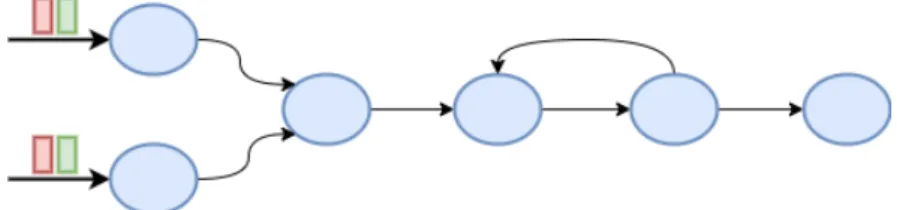
TheDataflow computational model expresses a computation as adirected graph (figure 2.1). Thenodes of the graph represent the operators executing arbitrary transformation on the input data. The edges of the graph represent the channels used by the operators to send messages and emit output data. Operators employ the shared-nothing principle and their potential interactions are explicitly expressed in the dataflow graph: dataflow edges are the only mean to exchange data and information. Channels typically provide First-In-First-Out (FIFO) delivery guarantees.

Apache Spark[12] successfully employed the dataflow model to tackle batch-processing at large scale, generalizing the first-introduced Map-Reduce model[10].

Apache Flink[2], Naiad [16] and Timely Dataflow [14] are stream-processing systems also based on the dataflow model.

2.2 Timely Dataflow

Timely [14] is a distributed stream processing system based on thetimely dataflow computational model, first introduced with Naiad[16]. It allows user programs to define dataflow

Figure 2.1:A sample dataflow graph. Blue nodes represent operators, black edges represent the inter-operator channels.

(13)

computations and executes them in a potentially distributed cluster of timely workers.

A dataflow graph is a (possibly cyclic) directed graph comprised ofnodes, the operators applying transformation on data, and edges, representing the channels where data are flowing along. Following the data-parallel paradigm, each worker in the timely cluster builds its own copy of the entire dataflow graph and then processes a portion of the input data. Workers operate asynchronously and independently from each other, exchanging data messages and progress information.

At the core of timely dataflow lies the progress tracking protocol, a distributed, asynchronous protocol which aims to track the progress of the computation and ensure some safety properties that guarantee the correctness of the produced output results.

Each message sent along dataflow edges carries a logical timestamp. Any partially- ordered data type can be used as timestamps, common examples are nanoseconds since the beginning of the execution (which can be employed to setup an open-loop experiment), or transaction numbers. More often that not, timestamps are integer tuples (whose partial order will be defined in section 2.3.1), as they fit naturally the concept of scoped and iterative dataflow graphs.

The progress tracking protocol tracksactive timestamps across the dataflow graph. The presence of active timestamps has implications on what input a certain operator might see in the future. Afrontier, a minimal set of incomparable, partially ordered timestamps, fully characterizes the set of active timestamps. Thus, we model active timestamps at operators input and output ports as frontiers. For each operator input, the corresponding input frontier constrains the possible timestamped-data that might be seen by that operator in the future: only data with a timestamp that is larger than any element in the frontier might ever be pulled from that input channel in the future. This is the essential safety property that is ensured by the progress tracking protocol.

Each dataflow operator is provided a capability for each output port. A capability, or rather a capability set, expresses the ability for that operator to emit data at that output port, carrying a timestamp larger or equal to any of the timestamps associated with its capabilities. Capabilities can be completelydiscarded, or downgraded over time as progress is made in the computation, affecting the corresponding output frontier.

The progress tracking protocol is extremely flexible and versatile, and can be employed to achieve diverse tasks that rely on the same safety property. Megaphone [15] is a library built on top of Timely to implement dynamic scaling and flexible state-management of operator state. Megaphone was entirely written in user-level code, only using primitives exposed by Timely, without needing to modify the underlying system. It provides a generic operator wrapper that performs state migrations across different worker instances of the same operator, relying only on the capabilities guarantees ensured by the progress tracking protocol.

In this work, we implement a fault-tolerance mechanism for Timely, again using only user-level library code. The design of Megaphone, having proved its effectiveness, inspired the design of this project and of the stateful operator - the generic operator which implements the fault-tolerance mechanism.

2.3 Concepts and Definitions

In this section we present in more details and formalize some of the core concepts behind Timely timestamp infrastructure, as we will rely on them thoroughly for our fault- tolerance mechanism. In particular, we describe whatfrontiers are and why they are the right abstraction to model progress in Timely dataflow computational model.

(14)

2.3.1 Partial Order

According to Wikipedia [22], “a partially ordered set consists of a set together with a binary relation indicating that, for certain pairs of elements in the set, one of the elements precedes the other in the ordering”.

At the core of Timely lies the concept of multi-dimensional timestamps: tuples of arbitrary partially ordered elements, typically integers. We define a partial order on multi-dimensional timestamps using the following definition of the≤operator.

Definition 1. Let t_x = (x₁, x₂, .., x_k) and t_y = (y₁, y₂, .., y_k) be two k-dimensional timestamps, then we sayt_x ≤t_y if and only if ∀i∈ {1, . . . , k}, x_i ≤y_i.

Note that this is not the lexicographical order of tuples, which would induce a total order on the set instead.

Lattice

Alattice [21] is a partially ordered set (S,≤) which, for each non-empty subset S⁰ of S, defines two elements: themeet (greatest lower bound) and thejoin(least upper bound) ofS⁰ [20].

Definition 2. Let(S,≤) be a partially ordered set, letS⁰ ⊂S and S⁰6=∅, then themeet of S⁰ is the greatest element m∈S such that ∀x∈S⁰, m≤x.

Definition 3. Let (S,≤) be a partially ordered set, let S⁰ ⊂S and S⁰6=∅, then thejoin of S⁰ is the smallest elementj ∈S such that ∀x∈S⁰, x≤j.

t₁ (3,7) t₂ (4,6)

meet(t₁,t₂) (3,6) join(t₁,t₂) (4,7)

timestamps ≤

Figure 2.2: Join and meet elements for two-dimensional timestamps.

Figure 2.2 shows an example for a two-dimensional timestamp scenario.

2.3.2 Frontier

Definition 4. Anantichainis a minimal (size-wise) set of mutually-incomparable partially- ordered elements.

A minimal antichain, or frontier, is an antichain which has been obtained by repeatedly adding elements to the set, and evicting comparable larger elements until the resulting set is again an antichain. Note that the final minimal antichain obtained depends on the set of elements only, not on the order in which they are inserted. The operation

(15)

of building a minimal antichain can be thought of as a function that maps a (multi)set of partially ordered elements to an antichain.

Example Consider the set S = {(2,15),(3,15),(7,9),(10,10)}, the corresponding minimal antichain is the set A = {(2,15),(7,9)}. (3,15) and (10,10) do not belong to the minimal antichain since (2,15)<(3,15) and (7,9)<(10,10).

We define the≤operator (and similarly ≥) for timestamps and frontiers as such:

Definition 5. Lettbe ak-dimensional timestamp, letf be a frontier made ofk-dimensional timestamps, then we say that t≤f if and only if ∃t⁰ ∈f, t≤t⁰.

Example Consider three timestamps t₁ = (3,4) t₂ = (3,16) t₃ = (3,14) and a frontier f ={(2,15),(7,9)}, thent1 ≤f,t2≥f andt3 is incomparable tof.

2.3.3 Frontiers as Partial Order

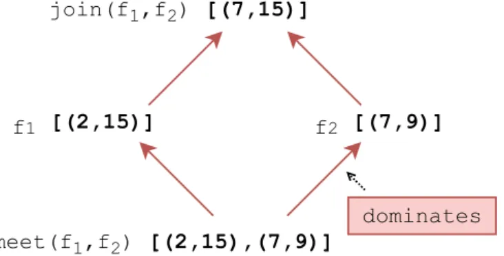
Definition 6. Let f1 and f2 be two frontiers, we say that f1 dominates f2 if and only

∀t₂ ∈f₂,∃t₁∈f₁, t₁ ≤t₂

Examples

f1={(2,15),(7,9)},f2 ={(3,16),(7,9)},f1 dominatesf2

f₁ = {(2,15)}, f₂ = {(7,9)}, f₁ does not dominate f₂, and neither the contrary (they are incomparable with respect to thedominate relation).

f1 [(2,15)] f2 [(7,9)]

meet(f₁,f₂) [(2,15),(7,9)]

join(f₁,f₂) [(7,15)]

dominates

Figure 2.3:Join and meet elements two-dimensional timestamps frontiers. Red arrows represent the dominates relation.

Using the dominates relation, we can define a partial order on a set of frontiers. As we can also define themeet and join frontier elements, it is also a lattice. Figure 2.3 shows themeet and join frontiers for the second example above.

We define themeet_frontiersandjoin_frontiersas functions that take an arbitrary number of input frontiers (of the same timestamp type) and return the meet and join frontiers respectively.

(16)

2.3.4 Using Frontiers to Track Progress

As already introduced in section 2.2, the progress tracker is arguably the most important component of the entire Timely infrastructure. The progress tracking protocol is an asynchronous, peer-to-peer protocol to which every worker participates and contributes to. Its ultimate goal is to provide guarantees about which timestamps an operator might have to process at its input channels in the future. This guarantee is provided by tracking active timestamps throughout the dataflow graph. Each operator port (i.e. input and output channel endpoints) is associated with a frontier. A frontier, comprised of n- dimensional timestamps, unambiguously defines an open manifold of the n-dimensional space (i.e. a potentially unbounded portion of the space). In simple terms, a frontier constrains active timestamps to all timestamps that are larger or equal to any of its timestamp-elements, and thus represents the ideal abstraction to model the progress in the computation.

2.4 The Fault-Tolerance Problem

Fault-tolerance is typically referred to as the ability of a system to continue to correctly operate in the presence of failures. What correctness means depends on the specific system and the guarantees it provides. For example, for a distributed database this could boil down to not lose part of the state (i.e. the result of write operations) when one of the servers fails. For such system, failing to fulfill the fault-tolerance requirements is likely to compromise its correctness in an irreparable way: some future queries, relying on part of the lost state, will return incorrect results.

Distributed stream processor are generally employed to perform data analytics on continuous streams of input data. The input streams are typically assumed to be a reliable source, whose content can be potentially replayed (e.g. Kafka topics [3]). In these terms, fault-tolerance for stream processors becomes an optimization problem, where the goal is not to protect unrecoverable state, but rather avoiding to repeat the whole computation from scratch in case of failure. Depending on the specific dataflow computation, re-computing the entire state from scratch might or might not be practical. Consider somewindowing operator (very common in streaming queries), if the size of the window is large (e.g. last 24 hours), then you would need to replay 24-hours-worth of data at the same input rate. Even worse would be to recompute state that depends on the entire history of the input stream, such as a simple non-windowed version ofWordCount.

One widespread approach to address this problem relies onrollback recovery. In rollback- recovery mechanisms, the state of the entire dataflow computation is periodically persisted to some durable storage, creating acheckpoint. In case of failure, one would recover the last persisted checkpoint and resume the computation since that point, thus avoiding the repetition of already-performed work. The distributed nature of the system makes the problem of creating aconsistent checkpoint of the dataflow state non-trivial: workers exe- cute asynchronously and independently, and message delivery is subject to unpredictable delays and network issues.

2.4.1 Limitations of the Existing Solutions

Some systems, such as Flink [6, 5], tweak the original algorithm presented in [8] to snapshot the state of the dataflow graph reflecting all the inputs up to a specific point in time (referred to as an epoch boundary). Such approach requires a significant amount of coordination between operators (and parallel workers) in order to determine when it

(17)

is safe to persist their state to durable storage. In particular, special marker messages are sent along the dataflow edges to signal the end of the current epoch and initiate the snapshot. Upon receiving the first marker, a stateful operator stalls and waits until a marker has been received on every input channel. Once all markers have been received, the stateful operator persists its state and forwards the marker to the downstream operators. Marker alignment imposes extensive coordination among operator instances and has been shown by the authors themselves in [5] that it results in several hundreds of milliseconds overhead to steady-state latency when the parallelism increases. Moreover, the approach requires special handling of cycles in the dataflow, which would cause the algorithm to deadlock otherwise.

Other Systems, like MillWheel [1], rely on an external reliable distributed database to persist the operator state and highly-available key-value store to provide the fault- tolerance guarantees. While this outsources most of the fault-tolerance-related concerns, accessing the state incurs a high-overhead, which affects steady-state latency significantly.

In the next chapter, we will present a novel mechanism that aims to solve the above- mentioned coordination problem, without relying on external fault-tolerant systems.

(18)

3 Fault-Tolerance Mechanism Overview

In this chapter, we present a high-level overview of our fault-tolerance mechanism, focusing on the novelty of the approach and how we believe it can address the shortcomings affecting existing solutions. We first give a definition of correctness in the context of fault-tolerance for stream-processors and then give the intuition of how it is achieved by our mechanism. We will also present the challenges to generalize the same mechanism to implement dynamic scaling of the cluster.

3.1 Correctness of the Mechanism

Below we report the main property that we wish to achieve. We say that if such property is achieved, then the mechanism iscorrect.

Correctness We want an execution subject to an arbitrary number of failures to be undistinguishable from a correct execution (where no failure has occurred) with respect to the application state and its emitted output¹.

A way to ensure the correctness property is to guarantee that every message is accounted for exactly-once. For example, in aWordCount dataflow, you want a word occurrence to be counted only once in the word-count accumulation maintained as the operator state.

Exactly-once delivery semantic is trivially achieved in a correct execution, simply because messages are sent only once and they are neither lost or dropped. In the presence of failures, one must ensure that the persisted state isconsistent with the input that will be processed after recovering. In other words, if we visualize the input stream as an ordered sequence of tuples, you want to recover a state that, for some index i, reflects all the effects of the portion of the input stream [0, i), and then process every single input tuple with index≥i.

3.2 Mechanism Overview

Most fault-tolerance mechanisms rely on persisting theapplication state to some durable storage, so that on failure the previous work is not lost, at least for the major part. What application state is defined to be, how and when is it persisted, and how is it useful on recovery, are the major design decisions that characterize a fault-tolerance mechanism.

As any non-trivial dataflow employs several stateful operators that need to persist their state and recover it after a failure, one approach could be to achieve correctness for the entire dataflow as a whole. One unfortunate consequence of this is that the different stateful operators would need tocoordinate when persisting their state. Referring to the example above, the would need to agree on the same indexi. As the mechanism is based on Timely timestamps, an indexiactually corresponds to a frontier.

1Note that if operators interact with the outside world (e.g. a distributed database) we do not require the mechanism to provide any specific guarantee on the state of the external system.

(19)

An alternative strategy, and the one adopted in our mechanism, is to guarantee correctness for each stateful operator independently, without coordinating them. We shift the focus from the entire dataflow to a single stateful operator. Our goal is to design an operator-local mechanism to persist the operator state that does not require coordination with its upstream/downstream operators and its parallel physical instances managed by other workers. The persistence mechanism, coupled with an asynchronous communication protocol, ensures that the correctness property (i.e. exactly-once delivery semantic) is achieved for the single operator instance. Achieving the property individually for every stateful operator guarantees that the property is achieved for the ensemble of stateful operators, the whole dataflow.

3.2.1 Incremental Operator State Persistence

Having removed any sort of coordination when persisting the state, each stateful operator is free to persist its state as a sequence of timestamped delta updates. We record the updates in an append-only data structure (theTrace data structure described in section 4.1) which has the characteristic of being multi-versioned, i.e. it can reconstruct the state at arbitrary points in time. Updates are gathered in batches and persisted via the durability subsystem.

3.2.2 Persistence Progress and Recovery Guarantees

A stateful operator asynchronously communicates to its upstream operators its persistence progress, i.e. up to which frontier (a point in time for possibly multi-dimensional timestamps) it has durably persisted its state. We call such frontier therecovery frontier of the stateful operator, as it corresponds to the frontier the operator would recover at in case of failure. If we want to draw a parallel with other systems, this corresponds to the time at which the last snapshot was taken for that operator. Two fundamental guarantees build upon the recovery frontier.

Recovery Guarantee 1 On recovery, an upstream operator will never be requested to replay output tuples with timestamp smaller than the recovery frontier of the stateful operator.

Recovery Guarantee 2 On recovery, an upstream operator must be able to replay all output tuples with timestamp larger or equal to the recovery frontier of the stateful operator.

A stateful operator is asynchronously communicated from its downstream operator the downstreampersistence progress, i.e. up to whichfrontier the downstream has consumed the output stream and has durably persisted its state reflecting the corresponding effects.

We call such frontier thedownstream recovery frontier, as it corresponds to the frontier the downstream operator would recover at in case of failure. Two fundamental guarantees build upon the downstream recovery frontier.

Recovery Guarantee 3 On recovery, a stateful operator will never be requested to replay output tuples with timestamp smaller than the downstream recovery frontier of the downstream operators.

(20)

Recovery Guarantee 4 On recovery, a stateful operator must be able to replay all output tuples with timestamp larger or equal to the downstream recovery frontier of the downstream operators.

This last recovery guarantee is the real challenge of the mechanism implementation. To fulfill it, we will rely on the multi-versioned data structure storing the operator state and the (not very limiting) assumption that one is able to reproduce output tuples from the operator state.

3.2.3 The Mechanism in a Nutshell

Each stateful operator incrementally persists its own state, requiring no coordination with other dataflow operators or peer workers. Each stateful operator tells its upstream operator up to which point it has durably persisted its state. Each stateful operator is told by its downstream operator up to which point the downstream has durably persisted its state. On recovery, a stateful operator requests all input tuples with timestamp larger or equal to its recovery frontier and replays all output tuples with timestamp larger or equal to the downstream recovery frontier.

3.2.4 A note on Coordination

Above we argued that our mechanism requires no coordination whenpersisting the state delta updates. However, in order to maintain the recovery guarantees in a distributed system, some coordination between workers must occur, and our mechanism in no exception.

In particular, coordination happens at the progress tracking level: persistence progress information are communicated using standard Timely inter-operator connections which heavily rely on the underlying capability system. When a frontier is communicated, it is aggregated among all parallel instance of the operator of all the workers to obtain a unique aggregate value (we will describe this in detail in the following chapter).

The novelty of the approach is that coordination has been removed from the critical path of state persistence and turned intoasynchronous aggregation of frontiers which has no effect on end-to-end latency.

3.3 Dynamic Scaling Overview

The fault-tolerance mechanism provides semantics for persisting operator state asynchronously and initializing a new computation from such previously-persisted state. We can leverage the mechanism for another system task: dynamic re-scaling of the cluster and load-balancing. We now describe how, by pre-partitioning the local operator state in sub-shards, they can be dynamically re-assigned to different workers in a process similar to failure recovery.

We pre-partition the operator state (i.e. a key-value collection) using a user-provided partitioning function. The partitioning function divides the operator state in non-overlapping shards, each containing only a subset of the keys. Shards represent the atomic unit of state that can be potentially re-distributed among the workers during a re-scaling operation.

A reconfiguration may grow or shrink a cluster, or re-assign subsets of the state. On reconfiguration, we briefly shut down the cluster, re-assign the state sub-shards according to the new configuration and resume execution. Except for the sub-shards re-assignment, this process is identical to failure recovery and does not require a separate re-scaling protocol.

(21)

The same technique can be also employed to change the routing function among workers for load-balancing or applying software patches. The only constraint imposed by the mechanism is that the persisted-state format must not be changed.

On an important note, we must ensure that the four recovery guarantees presented in the previous section are maintained even in the case of re-partitioning of the operator state. We will achieve such goal by adding an extraasynchronouscommunication channel between parallel instances of the same stateful operator, so that each operator instance is aware of the pace at which the other instances are persisting their state. The intuition is that the slowest operator instance determines what is the recovery frontier that must be considered when ensuring recovery guarantees. Note that this change has no impact on end-to-end latency, as the communication happens asynchronously and off the critical path.

(22)

4 Trace and FutureLog Data Structures

In this chapter we set the ground for presenting the design of the stateful operator, by introducing the Trace and FutureLog data structures – the backing stores for the operator state and fundamentals building blocks for the overall design.

We will first motivate their design presenting the requirements of the use-case and then explain the implementation details and the optimizations that improved upon the original prototype.

4.1 Trace Data Structure

We leverage the existing implementation of theTrace, a multi-versioned, LSM-like data structure, to incrementally store operator state changes. The existing implementation is part of the open-sourceDifferential Dataflowproject [13]. In this section we present our requirements for the operator state data structure, we describe the existing implementation, and detail the changes necessary to support our use case.

Below are listed the most important requirements that led to the design of theTrace data structure:

enable asynchronous, off-the-critical-path, incremental persistence of the operator state

optimized for a write-heavy workload

minimize the write-amplification of records (i.e. how many times the same record is rewritten)

natural integration with timely cornerstone concepts, in particular its timestamps- based progress tracking protocol

The above points suggested a Log-Structured Merge-Tree (LSM-Tree) [17] inspired data structure. The LSM-Tree is a disk-based data structure designed to provide very efficient insertion (and deletion) of records and low-cost indexing. Propagations of updates is deferred and batched, cascading the changes over a possibly multi-level hierarchy of in- memory-based and disk-based components. The propagation is performed following a merge-sort inspired algorithm, that aims to rewrite records only logarithmically many times (over the number of total records). LSM-Tree is a logically immutable append- only data-structure, in the sense that old record are not modified in place, but rather new records (carrying a larger timestamp) are batched and appended to it. This allows for very memory-friendly access patterns, thus increasing write efficiency and making it suitable for write-heavy workloads.

The Trace data structure is a multi-versioned append-only collection of (Key, Val, Time, Diff) tuples. It is multi-versioned, as one can reconstruct the state of the collection at different points in time, i.e. at different frontiers, by aggregating tuples with timestamp smaller to one such frontier. The trace is organized asbatches of tuples.

(23)

4.1.1 Batch

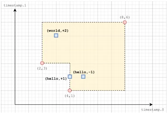
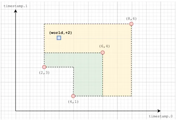
ABatch is a collection of (Key, Val, Time, Diff) tuples. Each batch is characterized by aDescription, which consists of three frontiers:

Thelowerfrontier represents aninclusive lower bound for the timestamps that can appear in the batch.

Theupperfrontier represents anexclusive upper bound for the timestamps that can appear in the batch.

The since frontier represents the frontier up to which updates within the batch might have beencompacted.

A batch maintains a few invariants. It is always¹ the case thatlowerdominates upper.

All tuples belonging to the batch must present aninitial timestamptsuch thatlower≤ t<upper, where≤is the timestamp-frontier relation defined in the background chapter.

While there is no restriction on its value, the since frontier provides a guarantee on the content of the batch: if tuples are accumulated up to some frontier F, such that sincedominatesF, then the reconstructed state is equivalent to the state that would be reconstructed if not compaction of tuples happened at all. This is a fundamental property that we will get back to and rely on thoroughly. There is no reason to be concerned if it does not make much sense for the moment.

(2,3)

(4,1)

(8,6)

(hello,+1)

(hello,-1) (world,+2)

timestamp.0 timestamp.1

Figure 4.1: Visual representation of a sampleBatch with two-dimensional timestamps.

Figure 4.1 shows a visual representation of the following sampleBatch:

1except in a very specific case of the recovery protocol, which will be described in a later chapter

(24)

B a t c h {

D e s c r i p t i o n { l o w e r : [(2 ,3) , (4 ,1)] , u p p e r : [(8 ,6)] , s i n c e : [ ( 0 , 0 ) ] } T u p l e s [(" h e l l o " , () , (4 ,2) , +1) ,

(" h e l l o " , () , (5 ,2) , -1) , (" w o r l d " , () , (3 ,5) , + 2 ) ] }

As timestamps are two-dimensional, we can visualize it on a cartesian plane, where the two axis represents the first and second timestamp coordinates, respectively. The yellow region, visually representing the[lower, upper)range, is the potential timestamp space for the tuples within the batch.

Compaction of Tuples

A batch supports a compaction operation on the tuples it contains. Thesince frontier represents the frontier up to which compaction of updates might have occurred.

A compaction operation up to some frontierFconsists of the following high-level steps:

1. Advance each timestampt<FtoF.

2. Aggregate all tuples with the sameKey,Valand Timeby the Diff field.

3. Maintain only those tuples with a non-zeroDiff field.

As an example, suppose we perform compaction of the sample batch above up to F = [(6,4)]:

B a t c h @ step 1 {

D e s c r i p t i o n { l o w e r : [(2 ,3) , (4 ,1)] , u p p e r : [(8 ,6)] , since: [(6,4)]}

T u p l e s [(" h e l l o " , () , (6,4), +1) , (" h e l l o " , () , (6,4), -1) , (" w o r l d " , () , (3 ,5) , + 2 ) ] }

T u p l e s [(" h e l l o " , () , (6,4), 0) , (" w o r l d " , () , (3 ,5) , + 2 ) ] }

T u p l e s [(" w o r l d " , () , (3 ,5) , + 2 ) ] }

Figure 4.2 shows a visual representation of the same sampleBatchafter the compaction operation has been performed. The green sub-region, delimited by the since frontier, indicates that any tuple within that timestamp region might have been compacted. In particular, tuples might present a timestamp value different from their original value, or, as in the example above, they might get cancelled out as theDiff accumulated to zero.

(25)

(2,3)

(4,1)

(8,6) (world,+2)

timestamp.0 timestamp.1

(6,4)

Figure 4.2: Visual representation of the same sampleBatch after compaction.

InternalBatch structure

What we have described so far are the abstract ideas of what a Batch is and how it should behave. The specific data structure storing the tuples depends on the specific implementation.

Certain operations (e.g. merging of batches, as we will soon discuss) would benefit from having the batchindexed in some way, so that look-ups within the batch are very efficient.

Moreover, as batches are immutable, they need to be indexed only once on creation. In the current implementation, batches are indexed first by Key, then by Value and finally byTime. They are stored in a custom trie-like data structure.

Iterate on the Tuples

Naturally, the batch exposes an interface to iterate over its content. Such iterator object is called aCursor. As there is no constraint on how the tuples are laid out in memory (e.g.

in one implementation they are stored as an ordered trie data structure), the interface follows theinternal iteration pattern via themap_timesfunction of theCursor. In other words, you provide a closure that will be invoked for each tuple of the batch. It is important to point out that a cursor iterates on thecurrent content of the batch, which might have been compacted.

4.1.2 Merging Batches

In the previous subsection we described the structure of batches. A trace manages a contiguoussequence of batches, where eachlowerfrontier is equal to the previous batch’s upperfrontier (if any).

In order to bound the amount of memory and disk space necessary to store the collection batches, the collection supports progressive summarisation and merging. A collection-

(26)

widedistinguish_sincefrontier controls for which timestamps the trace must maintain detailed change information. For all timestamps smaller than the distinguish_since frontier, the trace can replace batches so that the accumulation of the trace up to distinguish_sinceremains equivalent.

The trace can decide tomerge adjacent batches into a new batch, essentially eliminating the “inner” boundary. As thedominates relation is transitive, the lower frontier of the merged batch still dominates the upper frontier of the merged batch, thus maintaining the invariance. Thesince frontier of the resulting merged batch is computed as follows:

merged_batch.since = join_frontiers(batch1.since, batch2.since) The intuition behind this is that, in order to not violate the since frontier guarantee about the reconstructed state, the since frontier of the merged batch must be larger than thesincefrontiers of the batches being merged.

Suppose this is not the case, one of the batches might have advanced the timestamp of tuples whose original timestamp is larger than the newsince frontier, clearly violating the safety guarantee.

During a merge operation, the trace can also decide to allow compaction of the tuples within the merged batch, as explained in the previous section. The frontier used for compaction is controlled by the user code owning the trace, we call it thedistinguish_since frontier.

Thesincefrontier guarantee of batches can be generalized for thedistinguish_since frontier of traces: if tuples are accumulated up to some frontierF, such thatdistinguish_since dominates F, then the reconstructed state is equivalent to the state that would be reconstructed if not compaction of the underlying batches happened at all.

Allowing the trace to compact the underlying batches up to some frontierF, we are giving up thedistinguish_sinceguarantee for any frontier dominating thedistinguish_since frontier. Intuitively, this means that we are able to iterate over and distinguish the indi- vidual original tuples (using aCursor on the trace) only since thedistinguish_since frontier.

While compacting the trace reduces its capability of being “multi-versioned”, it is a necessary action to perform in order to prevent the trace from growing indefinitely.

Merging batches plays also an essential role, as compaction is possible only within a batch itself.

Merging Strategy

To characterize a merging strategy we essentially want to define:

which batches do we merge

how much effort do we put in performing such merges.

For the first point, our goal is to minimize the write-amplification of each tuple, as it in turns implies minimizing the overhead of merging. A merge-sort inspired strategy allows us to merge batches logarithmically many times in the number of inserted records, by repeatedly merging batches of similar sizes². When two batches are being merged, they are also compacted up to thedistinguish_since frontier.

2every batch size is rounded to the next power of two for the purpose of the comparison

(27)

When a merge operation is initiated, it is not necessarily taken to completion synchronously. In other words, the merge is likely to not be completed entirely during the same function call that initiated the merge, but rather the work is performed progressively and proportionally on the size of the new batches being inserted in the trace. Spread- ing the merging overhead over time avoids spikes in latency and achieve a more regular behavior.

4.1.3 Persisting Batches

If a timely worker fails, all its in-memory data structure are lost. A natural requirement for a fault-tolerant system is the ability to persist the state of the application to some durable storage. On recovery, we would access that storage and recover the work that was already done, or at least part of it.

TheTrace data structure will backup the state maintained by thestatefuloperator, the generic operator implementing the fault-tolerance mechanism, introduced in the following chapter. As such, it will interact with somedurability subsystemvia a well-defined interface in order to persist the produced batches to durable storage.

4.2 FutureLog Data Structure

Timely operators are provided withcapabilities, expressing their ability to produce output tuples carrying a certain timestamp. An operator can produce an output tuple at timestamp tout if and only if it holds a capability for a timestamp tcap such that tcap ≤ tout. In other words, an operator is effectively allowed to produce output in the future as a consequence of something that happened in thepresent.

This flexibility comes very handy in multiple occasions. For instance, implementing a sliding-window for a counting problem (e.g. the implementation of NexMark query 5 in the Evaluation chapter) is as simple as emitting a positive delta for the current time t, and the corresponding negative delta for the future timet+window size.

In order to not give up this flexibility, we must explicitly distinguish between the time at which a message was produced and the actual time a message is supposed to be delivered. In particular, the operator state at some frontier f must include all those future messages that were produced at some timestamp t_produced < f and have some actual future timestampt_actual≥f.

In this section we describe the design and implementation of theFutureLogdata structure. Its purpose is very simple: store (and durably persist) future messages until they become “present” and ready to be processed by the operator.

4.2.1 A Collection of Batches

Similarly to the Trace data structure, the FutureLog exposes an interface to append batches of future messages. AFutureMessageis simply the message payload augmented with the actualfuture timestamp (the produced timestamp is implicit and determined once the message is received). The batches are characterized by two frontiers and one timestamp:

Theproduced_lower frontier represents an inclusive lower bound for theproduced timestamps that can appear in the batch.

Theproduced_upper frontier represents anexclusive upper bound for theproduced timestamps that can appear in the batch.

(28)

The actual_upper_bound timestamp represents the maximum actual timestamp that is present in the batch.

The FutureLog allows garbage collection of batches up to some frontier. A batch can be garbage collected if and only if its actual_upper_boundis smaller than the provided frontier, meaning that all the messages it contains are older than the garbage collection frontier.

4.2.2 Message Stash and Notificator

Each appended batch is not stored as it is: each message contained in the batch is stashed away in a map indexed by theactualtimestamp and a notification for that time is setup accordingly, using a Timely FrontierNotificator. When the future message is not in the future anymore, a notification is delivered, and the message is unstashed and made available to the user using the data structure. Storing the content of the batches in a map allows for efficient insertion and retrieval of messages, which would not be possible if they were kept in memory using the batch layout.

4.2.3 Persistence of Batches

Similarly to the Trace data structure, the FutureLog persists the appended batches to some durable storage. A straightforward solution would be to simply persist every single batch that has been appended. The initial prototype employed this simple approach, but as the amount of produced batches was extremely large at high rates, the durability subsystem was overwhelmed and unable to persist all the batches at a reasonable pace.

We prototyped an alternative approach, with the goal of self-regulating the amount of batches that the durability subsystem has to persist, which we now describe.

Optimized Persistence of Batches

The durability subsystem informs the FutureLog what is the upper frontier of the last batch it has successfully persisted. If the durability subsystem is keeping up well, the last persisted batch will be just a few batches behind the last appended batch. If the durability subsystem is running behind, it will have a non-negligible amount of batches yet to persist.

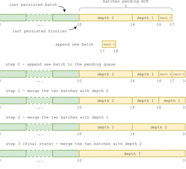
In order to reduce the amount of batches to persist by the durability subsystem, the FutureLogkeeps track of the batches pending acknowledgment and merges them. Batches are merged in logarithmic fashion, in order to minimize the write-amplification of each future message. Batches are associated with a depth, representing their level of merging (i.e. their depth in the logical tree of the merges), and only adjacent batches with the same depth will be merged.

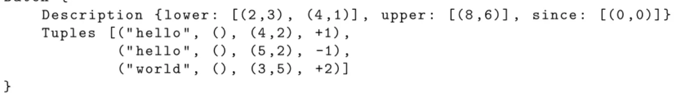
Figure 4.3 shows an example of the merging process in action, for a single-dimensional timestamp scenario. The green batches in the figure have been persisted already by the durability subsystem, and they are not kept in memory anymore (only showing them to give some context): as their content has been already stashed in the map, they are not useful anymore. When the new batch is appended to theFutureLog, a cascade of merges is triggered. The intermediate merged batches are not sent to the durability subsystem, but only the last produced at the end of the merging process (the batch with depth 3).

Note that the batches have been assumed to have constant size of one time unit for the sake of explanation, but that is not necessarily the case for real executions. Moreover,

(29)

0 ... 10 last persisted batch

last persisted frontier

depth 2 depth 1 ^{depth 0}

depth 0

14 16 17

append new batch

17 18

step 0 - append new batch to the pending queue

0 ... 10

depth 2 depth 1 ^{depth 0}

14 16 17 18

step 1 - merge the two batches with depth 0

0 ... 10

depth 2 depth 1 depth 1

14 16 18

depth 0

step 2 - merge the two batches with depth 1

0 ... 10

depth 2 depth 2

14 18

step 3 (final state) - merge the two batches with depth 2

0 ... 10

depth 3

18 batches pending ACK

Figure 4.3:Sample merging process of the FutureLog pending queue.

the merging strategy is independent of the time range spanned by each batch, and relies only on the depth of the batches.

The next time the durability subsystem processes new batches, it will be presented with some overlapping batches, as shown in figure 4.4. Note that those batches were produced during previousappendoperations, but were never processed by the durability subsystem. The durability subsystem will store only non-overlapping batches, while still ensuring that the whole contiguous time range is covered. In this simple example, only the batch with depth 3 will be persisted.

This optimization gave substantial benefits to the overall performance of the system, reducing steady-state end-to-end latency by a significant factor and the latency spike on recovery by one second. It has the nice self-regulating property that, the more the durability subsystem is struggling (thus reporting an old last_persisted_frontier), the more merges will be performed by theFutureLog, resulting in less batches to persist.

(30)

depth 0

depth 1 depth 0

depth 1

depth 2 depth 0

depth 1 depth 0

depth 3

Figure 4.4:The collection of batches received by the durability subsystems (visually ar- ranged to reflect the spanned time ranges). Only the blue batch with depth 3 will be persisted.

(31)

(32)

5 The stateful Operator

In this chapter we describe the design and implementation of the stateful operator.

Thestatefuloperator implements the fault-tolerance mechanism, hiding its complexity by providing a generic interface and defining clear operator boundaries. We use the TraceandFutureLogdata structures introduced in the previous chapter, as fundamentals building blocks to maintain operator state. We will provide a detailed description of the stateful operator interface, along with a working WordCount example. We will then dive into the inner workings of the operator, and finally generalize its design to allow re-partitioning of its state to perform dynamic scaling.

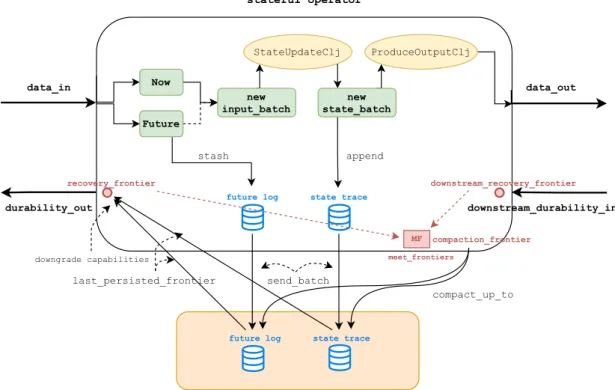
Figure 5.1 shows an abstract representation of the operator structure. The reader is invited to refer to it as we introduce new concepts in the following sections.

5.1 stateful Operator Input and Output Connections

Figure 5.2 depicts thestatefuloperator input and output connections for its one-input- one-output version.

data in is the input data stream. Its type is anenumwith two variants,NowandFuture.

Each timely message moving along dataflow edges is associated with the timestamp at which is was produced. In vanilla timely, such timestamp is arbitrary, as long as you hold a capability for it. In order to not give up this flexibility, but still be able to determine when a message was produced (a requirement for any recovery protocol), we need to model this explicitly. The Now variant represents a message whose actual timestamp is the timestamp at which it wasproduced. TheFuturevariant represents a message which is produced at a certain timestamp, but with a different (future)actual timestamp, which is stored explicitly alongside the message. Both variants wrap the message - a key-value pair (K1,D1). Input messages are routed among workers according to a user-supplied exchange strategy.

data out is the output data stream. Its type is arbitrary.

downstream durability in is the durability signal that downstream operator(s) con- suming the output stream are sending back to the stateful operator. Semantically, it indicates up to which point the downstream operator(s) has processed the output stream and durably persistedits effects. Its type is the Rust unit type(): nothing is actually sent along the dataflow edge, but rather we leverage built-in features of the progress tracker to make the information available (more on this later).

durability out is the durability signal that the stateful operator is sending to its upstream operator. Similarly to the downstream signal, it indicates up to which point thestateful operator has processed the input stream and durably persisted its effects.

Its type is also the unit type.

(33)

data_in Now Future

new input_batch

StateUpdateClj

new state_batch

ProduceOutputClj

data_out

future log

downstream_durability_in state trace

durability_out

recovery_frontier downstream_recovery_frontier

stash append

future log state trace send_batch last_persisted_frontier

Durability Subsystem

compaction_frontier MF

compact_up_to stateful operator

downgrade capabilities meet_frontiers

Figure 5.1:stateful operator structure

stateful

data_in data_out

downstream_durability_in durability_out

Figure 5.2: statefulinput and output connections

(34)

1 impl<G, D1> Stateful<G, D1> for Stream<G, Message<G::Timestamp, D1>>

2 where G: Scope, D1: ExchangeData + Ord {

3

4 fn stateful_unary_frontier<

5 D1K: ExchangeData + Ord, // input key

6 D2K: ExchangeData + Ord, // state key

7 D2: ExchangeData + Ord, // state value

8 D3: ExchangeData, // output type

9 KeyExtractor: Fn(&D1) -> D1K + Clone + 'static,

10 KeyHasher: Fn(&D1K) -> u64 + Clone + 'static,

11 StateUpdateClosure: FnMut(

12 &[G::Timestamp], // input frontier

13 &OrdValBatch<D1K, D1, G::Timestamp, i32>, // input batch

14 &mut StateBatchBuilder<D2K, D2, G::Timestamp, i32>

15 &TraceAgent<D2K, D2, G::Timestamp, i32>, // current state

16 ) + 'static,

17 ProduceOutputClosure: FnMut(

18 &mut dyn FnMut() -> Option<(D2K, D2, G::Timestamp, i32)>,

19 Option<(StateCursor<D2K, D2, G::Timestamp>,

20 &StateStorage<D2K, D2, G::Timestamp>)>,

21 ) -> HashMap<G::Timestamp, Vec<Message<G::Timestamp, D3>>> + 'static,

22 >(

23 &self,

24 name: &str,

25 key_extractor: KeyExtractor,

26 key_hasher: KeyHasher,

27 downstream_durability_in_stream: &Stream<G, ()>,

28 durability_context: DurabilityContext,

29 state_update_clj_builder: impl Fn() -> StateUpdateClosure,

30 produce_output_clj_builder: impl Fn() -> ProduceOutputClosure,

31 )

32 -> StatefulOut<G, D3> where G::Timestamp: Lattice { ... }

33 }

Listing 1:Function prototype of stateful unary frontier

5.2 stateful Operator Interface

Listing 1 shows the signature of the stateful_unary_frontier: the one-input-one- output version of the abstractstatefuloperator. The many template parameters might look a bit daunting, but it is not as complex as it looks. Let us analyze it piece by piece.

First, we declared a new traitStatefulwith a single methodstateful_unary_frontier and we implemented it for the timelyStreamtype. Messageis theenumwith two variants, Nowand Future, that has been introduced before. All key and value types are required to be thread-safe and serializable, thus we mark them asExchangeData- the timely trait to express these constraints. We ask the user to provide a few closures, which will then be used as building block in the generic implementation.

KeyExtractor extracts the input key D1K from the input data D1. We do not require the input stream to be an explicit stream of key-value pairs, but rather something that can be treated as such.

(35)

KeyHasher maps the input key D1Kto an integer value that will be used in the routing function to shuffle input data among workers.

StateUpdateClosure implements the core operator logic that processes new inputs and updates the operator state. The closure expects four input parameters:

the current input frontier

the new input batch to process

a mutable reference to a batch builder: an append-only collection of update tuples in the differential format (key-value pairs associated with a timestamp and a multiplicity)

a read-only handle to access the current state

ProduceOutputClosure emits the output corresponding to a new batch of state updates.

An important requirement is that the state must contain enough information for the closure to produce the output stream. The closure expects two input parameters:

an iterator on the new state updates (i.e. a closure to be invoked multiple times)

an optional read-only cursor on the current state 5.2.1 A WordCount Example

The description of the interface above can be probably better understood by looking at a simple example. Listing 2 presents a possible implementation of aWordCount dataflow.

In this specific counting problem, we can leverage the format of differential collections to achieve an efficient state encoding: (word, (), timestamp, diff), wherediff represents a variation in the count at a specific timestamp. TheStateUpdateClosuresimply emits, for each word in the input batch, a state update tuple in the format just described.

TheProduceOutputClosureemits, for every timestamp and for every word whose count changed at that timestamp, the updated count. To achieve this, we iterate over all new state updates, initialize the count with the content of the last recorded value in the operator state and then keep accumulating the diffs to it. Importantly, we rely on the fact that the get_next_updateclosure returns update tuples grouped first by word, then by increasingtimestamp.

Finally, we inspect the output (word-count pairs) and connect the durability signal. As theinspect operator is a stateless operator, it has nothing to persist or recover. Thus, we convert its output to an empty stream and use it as the durability signal. Intuitively, this means that we are only interested in printing the tuples.