Divergence Corrections in the Numerical

(1)

Divergence Corrections in the Numerical

Simulation of Electromagnetic Wave Propagation

F. Kemm

^∗

C.-D. Munz

^∗^†

R. Schneider

^†

E. Sonnendrücker

^‡

May 31, 2000

Abstract

Besides evolution equations the mathematical models for problems with electromagnetic waves also contain divergence constraints for the electric or magnetic

£elds. Due to the approximation errors in these constraints these errors may increase during numerical simulation in time and produce unphysical solutions. This can be avoided by coupling the evolution equations with the divergence constraints. The numerical simulations are then based on this constrained formulation of the underly- ing equations. In this paper we review this idea and its applications. A simple model problem shows the behaviour and properties of different approaches. Extensions for the MHD-equations are proposed.

1 Indroduction

Electro-magnetic wave propagation is mathematically modelled by the Maxwell equations. This system consists of two hyperbolic equations and two divergence constraints.

The hyperbolic equations

E_t−c²∇×B = −1 ε0

j, (1.1)

B_t+∇×E = 0 (1.2)

are evolution equations for the electric £eld E and the magnetic induction B, usually called Maxwell’s and Faraday’s law. Here, j denotes the current density, c is the speed of light,

∗Universität Stuttgart, Institut für Aerodynamik und Gasdynamik

†Forschungszentrum Karlsruhe, Institut für Hochleistungsimpuls- und Mikrowellentechnik

‡Universite Louis Pasteur, Institut de Recherche Mathématique Avancée

(2)

andε0is the dielectric constant which are related byε0·µ₀·c²=1, where µ₀denotes the magnetic permeability. The elliptical part of the Maxwell equations are given by the laws

∇·E = 1 ε0

ρ, (1.3)

∇·B = 0, (1.4)

whereρdenotes the charge density. Any solution of (1.1)-(1.4) satis£es the basic physical principle of charge conservation which reads as

ρt+∇·j=0. (1.5)

This equation is obtained by applying the divergence operator to (1.1), time differentia- tion to (1.3) and combining both results. Due to the fact that the curl of any vector £eld is divergence-free results in the conservation equation (1.5). Existence, uniqueness and stability of solutions may be considered by applying techniques of semigroup theory to the hyperbolic evolution equations, see [4]. Such an existence proof is then stated in the following way. If the initial data E₀, B₀satisfy the divergence constraints (1.3), (1.4), and if the functionsρand j satisfy (1.5) are given, then a solution E, B of (1.1), (1.2) exists that satis£es the divergence constraints (1.3), (1.4) for all times. We do not want to go into details at this point and omit to state the regularity of the solutions. For a bounded domain we need in addition appropriate boundary conditions for E, B.

Now we consider the numerical simulation. If initial data E₀, B₀ are given, then the approximation of the hyperbolic evolution equations by some numerical scheme, such as a £nite difference (FD-), £nite element (FE-) or £nite volume (FV-) scheme gives a procedure to calculate approximate values for the electric and magnetic £elds for all times.

But the situation is different to this mentioned above. Even, if (1.3) and (1.4) are satis£ed initially, the validity of the divergence constraints for all times can, in general, not be expected. Two kinds of errors may occur. The £rst is that a discrete divergence operator applied to a discrete curl operator may give the zero up to some approximation error only.

The second kind of errors may be introduced by the current density j. In the existence proof for the Maxwell equations it is assumed thatρand j are given functions satisfying (1.5). For certain problems the charge and current density are functions of the £elds itself and the charge conservation equation may be satis£ed up to an approximation error only.

In both cases, we cannot longer assume that (1.3), (1.4) are automatically satis£ed for all times as valid for the exact solution. Errors of the divergence constraints may increase during the calculation and strongly falsify the numerical results. Such phenomena in numerical calculation have been described for Maxwell equations, for MHD-equations, and for Maxwell-Vlasov equations, see [2, 3, 7, 9].

To avoid the £rst kind of errors, shortly named the div-curl-errors, special schemes have been constructed in the past. A FD-scheme without div-curl-errors has been proposed by Yee [16]. It uses a staggered grid where the different components of the £elds are calculated at different spatial and temporal locations. The extension to curvilinear structured staggered grids has been performed by Holland [5]. From a more general point

(3)

of view, the construction of the grid and approximation satis£es the important vector iden- tities is, of instance, considered by Hyman and Shashkov [6]. Within the FE framework the so called edge elements have been constructed where the divergence constraints are incorporated in the £nite element spaces (see Nédélec [13]). For a review of their ad- vantages and drawbacks we refer to Mur [12]. FV-schemes that satisfy the div curl=0 condition have been proposed by Madsen and Ziolkowski [8] and Weiland [15]. Here, the integral formulation of the evolution equations is obtained by using Stokes theorem and a staggered grid arrangement.

In this paper we follow another path very recently investigated in ([10]): There a mathematical model is introduced which couple the evolution equation with the divergence conditions by appropriate chosen differential operators. This generalised Lagrange multiplier (GLM) system may be considered as an extension of the constrained formulation of the Maxwell equations [1]. Standard correction techniques proposed in the literature are obtained as special cases of the numerical approximation of the GLM equations.

2 A constrained formulation of the Maxwell equations

In the cases where divergence errors or/and charge conservation errors appear in the numerical approximation, the Maxwell equations (1.1)-(1.4) are over determined and no exact solution exists. Solving the hyperbolic evolution equations these errors would not decrease rather then are pronounced during the calculation. The divergence constraints have to be taken into account in such a way that the numerical solution has to be enforced to be a good approximation of all equations, not the hyperbolic part only. In the following we replace the mathematical model established by the Maxwell equations by an approximate model whose solution allows charge conservation or/and divergence errors ([10]).

This GLM model system is given by

E_t−c²∇×B+c²∇ φ = −1 ε0

j, (2.1)

Bt+∇×E+∇ ψ = 0, (2.2)

g(φ,φt) +∇·E = 1 ε0

ρ, (2.3)

h(ψ,ψt) +∇·B = 0, (2.4)

where g and h are continuous functions ofφ, φt andψ, ψt respectively. The additional variables couple the divergence constraints to the hyperbolic evolution equations.

For brevity we restrict our discussion £rst to the case of charge conservation errors and discuss (2.1) and (2.3) only. A simple choice for the till not speci£ed function g is g≡0. This means that φis a Lagrange multiplier which couples the Ampère’s with the Gauss’ law. This has been proposed by Assous et al. [1] and mathematically justi£ed in a rigorous way. They called this approach a constrained formulation of the Maxwell equation and used it as the mathematical model for a FE approximation. A fractional step procedure may also be applied: First, the electric and magnetic £elds are calculated from

(4)

solving (2.1) and (2.2), then the £elds are corrected by the Lagrange multipliers according to the divergence constraints. This is known as the projection or Boris correction [2]. For zero-divergence conditions the correction step states the Helmholtz decomposition of the

£elds into a curl-free and a divergence-free part. In the numerical computation this is performed solving the Poisson equation:

∆ φ=− 1

ε0c²(ρt+∇· j) (2.5)

for the correcting potentialφ. This approach of course can be combined with any numerical scheme by performing the correction in a subsequent step. We call the yet mentioned approach the elliptic correction because the variableφcarries the charge conservation errors and is determined by the elliptic equation (2.5).

Another choice for the function g may be g(φ) = ^φ_β where β is a positive constant.

Instead of (2.5) the equation for the correcting function is now given by the parabolic one φt−βc²∆ φ= 1

ε0

(ρt+∇·j). (2.6)

This means that a local accentuation of errors are prevented by smoothing them out. An explicit approximation of this divergence correction approach - known as pseudo-current method and called in this contest as parabolic correction - has been proposed by Marder [9] and has been improved by Nielson and Drobot [14] and Langdon [7].

The choice g(φ) = _α^φ^t2 gives a hyperbolic correction method where the correction func- tionφsatis£es the inhomogeneous wave equation

φtt−α²c²∆φ= 1 εo

(ρt+∇·j). (2.7)

Local divergence errors are transported out of the computational domain with £nite speed αc. Moreover, it can be shown that the GLM model along with appropriate initial and boundary data and under usual regularity conditions admits a unique solution. A fur- ther result for the GLM system is that the energy norm is uniformly bounded in time if absorbing boundary conditions are imposed onφ. This guarantee that divergence errors do not increase in time and that both (1.1) and (1.2) are approximately satis£ed by the GLM model during the temporal computation. A numerical method based on the evolution equations only does possess this property. A numerical method only based on the hyperbolic evolution equation (2.1)-(2.2) clearly does not ful£l this condition.

3 A simple test problem

The simplest problem where the situation described above may occur is the system

u_t =0, ∇·u=0. (3.1)

(5)

If the initial data for u are divergence-free, then a solution of (3.1) exists. In the case, where the divergence of the initial data are non-zero at some points, then the problem (3.1) is over determined. The solution of the evolution equation only would preserve the divergence errors for all times. Now, we replace (3.1) by the approximate model

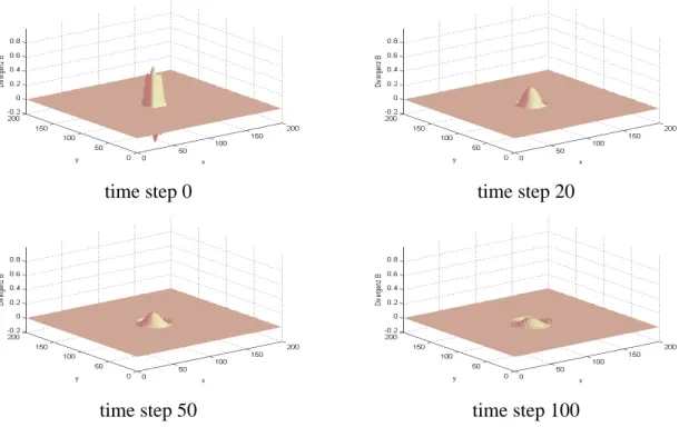
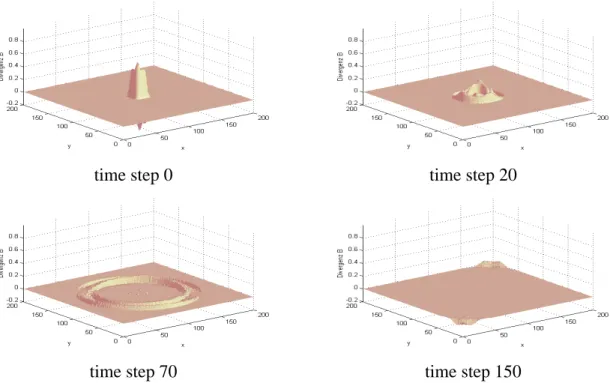
u_t+∇ φ=0, ∇·u+g(φ) =0, (3.2) whereφ is the additional degree of freedom. In that case we can get solutions of (3.2) where divergence errors decrease in time and, furthermore, a divergence-free stationary state is obtained. In the following we compare numerical results for the parabolic (g(φ) = φ), the hyperbolic (g(φ) =φt) and the mixed hyperbolic-parabolic (g(φ) = _α¹2φt+¹_βφ) ansatz. In the case of parabolic correction (cf. £gure 1) we discretize the £rst equation by forward differences in time and central differences in space. The second equation is discretized with central differences in space on the new time level. In each time step we solve the two discrete equations, one after the other and obtain an explicit procedure. A similar procedure can be deduced by performing a div-operation to the second and inserting the result into the £rst equation. For the hyperbolic ansatz (cf. £gure 2) we apply the Courant-Isaacson-Rees scheme to the system (3.2), which for this simple linear case is equivalent to any £rst-order upwind FV scheme, and can easily extended by dimensional splitting techniques for the two dimensional situations. In the mixed hyperbolic-parabolic (cf. £gure 3) case we reformulate the equations into a hyperbolic system with a source term and apply usual splitting methods. For every time step we £rst solve the hyperbolic part with the same scheme as for the purely hyperbolic correction and then the in¤uence of the source is computed. This second step is a simple ordinary differential equation that can be solved exactly.

The numerical results show the typical properties of the solution for the different types of correction methods. As expected for the elliptic correction procedure, the divergence error vanishes within one iteration cycle (not shown here). The parabolic correction intro- duces a smearing of the initial errors. The constantβhas been chosen as large as possible according to the parabolic stability condition for explicit schemes. In the hyperbolic approach the errors propagate out to the boundary of the domain. The wave velocityα has been calculated by the CFL-stability condition. For the value ofα=4.5 an additional dissipation has been switched on. The numerical results of this hyperbolic-parabolic approach is shown in £gure 3 for different values of β. Clearly, these results reveal the increase of the hyperbolic character for large values ofβ.

4 A constrained formulation of MHD-equations

Now we combine the constrained Maxwell equations with the ¤uid dynamic equations to derive a constrained form of the ideal MHD System. Usually one takes the Euler equations, plugs the Lorentz force into the momentum equation as well as the electromagnetic energy into the energy equation and expresses the evolution equation in terms of the magnetic £eld B and the ¤uid variables. The momentum equation with the Lorentz

(6)

time step 0 time step 20

Figure 1: Temporal evolution of the parabolic correction approach force term reads as

ρdv

dt = j×B−∇p, (4.1)

where quasi-neutrality is assumed. In the unit system where µ₀is equal to one and under the assumption that the displacement current is small compared to the spatial variation of B, the electric current obtained from Ampère’s law is

j=−∇×B.

Inserting this expression into (4.1) yields for the momentum equation the expression ρdv

dt =−∇(p+B²

2 ) + (B·∇)B. (4.2) Obviously, there is no in¤uence of the divergence constraint to this equation. In the non- relativistic case the electric £eld can be easily expressed in terms of the magnetic £eld and the ¤uid velocity

E=−v×B, (4.3)

known as Ohm’s law of ideal MHD. This has been also used for eq. (4.1).

Since a dimensional analysis for the MHD equations reveals quasi-neutrality (ρel.≡0), the evolution equations of the magnetic induction may be expressed according to

B_t−∇×(v×B) +∇ψ=0. (4.4)

(7)

Figure 2: Divergence error propagation obtained with the hyperbolic correction at different time steps

beta=1 beta=10

beta=100 beta=1000

Figure 3: Divergence error pro£le computed with the hyperbolic-parabolic correction after 10 time steps for £xedα(α=4.5) and differentβ

(8)

Using this constrained formulation of the magnetic £eld induction to compute the evolution of electro-magnetic energy we get

e_t+∇·

·

(e+p+1

2B²)v−B(v·B)

¸

=−B·(∇ψ). (4.5)

An additional term appears on the right hand side which is a consequence of the constrained formulation of the Maxwell equations. Under the considered constrained formulation, the resulting MHD system in conservation form reads as

ρt+∇·(ρv) =0, (4.6) (ρv)t+∇·(ρv·v^T+ (p+1

2B²)I−B·B^T) =−(∇·B)B, (4.7) B_t+∇·(v·B^T −B·v^T +ψI) =0, (4.8) e_t+∇·

·

(e+p+1

2B²)v−B(v·B)

¸

=−B·(∇ψ), (4.9)

g(ψ) +∇·B=0, (4.10)

manifesting a set of nine equations for nine unknowns (p= (1−γ)ρe). For a FV scheme of the MHD equations a central building block is often an approximate Riemann solver by which nonlinear wave propagation is incorporated into the numerical ¤ux calculation.

This fact establishes the robustness and the shock-capturing property of those schemes.

Locally the wave propagation at the edges between two adjacent grid zones into the normal direction is considered. The solution of the local one-dimensional Riemann problems is then used for the numerical ¤ux computation. The ideal MHD model in one space di- mensions spoils down to a system of seven equations, while the magnetic £eld into normal direction is restricted to be constant across the edge. This is, of course, in general not valid and the value of the normal B-component is set to be the arithmetic mean value.

This procedure is then combined by a subsequent projection correction step to obtain the divergence-free condition for B. In the constrained formulation proposed the correction of the divergence errors is automatically included. Besides the two additional eigenvalues

±ch, it is easy to show that the constrained system in one space dimension has the same eigenvalues as the usual MHD equations. In ascending order, the resulting eigenvalues read as

λ1=−c_h, λ2=u−cf, λ3=u−cA, λ4=u−cs, λ5=u,

λ6=u+c_s, λ7=u+c_A, λ8=u+c_f, λ9=c_h, where the abbreviations

c_A = |b1|, (4.11)

c_f = s

1 2

µ

a²+b²+ q

(a²+b²)²−4a²b₁²

¶

, (4.12)

cs = s

1 2

µ

a²+b²− q

(a²+b²)²−4a²b12

¶

(4.13)

(9)

with

bi= s

B²_i

ρ b²= B²

ρ a=

rγp

ρ (4.14)

are used. Inspecting A(q)−λiI for i=2, . . . ,8 more closely, one recognises that the sys- tem of eigenvalues does not becomes much more complicated. Because c_his constant, one can easily £nd out that every eigenvector of A(q)has a zero in the £fth and the ninth component. Now the £fth and the ninth lines of the matrix only have entries in the £fth and the ninth column. Hence, to each eigenvector r= (r1, . . . ,r7)^T of the seven one-dimensional MHD waves corresponds an eigenvector matrix ˜r= (r1, . . . ,r4,0,r₅, . . . ,r8,0)^T of A(q).

So none of the waves travelling with wave speedsλ2, . . . ,λ8 carries a change in B₁ orφ and none of the corresponding wave strengths is proportional to a jump in B₁orφ.

One problem in the hyperbolic approach are ¤ux terms on the right hand side of the conservation form, that play the role of sources. In the numerical approximation rounding and discretization errors may lead to violation of charge conservation even if the initial values are divergence free. Using the GLM Maxwell system not for the derivation of the GLM-MHD model but for the correction in the usual MHD equation context avoids that source terms occur. The considerations for the eigenvalues and eigenvectors are also valid in this case. The only difference is in the eigenvectors to the eigenvalues±ch.

5 Conclusions

The constrained formulation of the Maxwell equations gives a uni£ed approach to divergence correction techniques. The Boris projection method [2], called the elliptic approach in our formulation, needs the numerical solution of a Poisson equation. This needs a lot of computational effort and becomes cumbersome, especially, in combination with an explicit treatment of the hyperbolic £eld equations. But, it might be not necessary to apply the projection step at each time level, but only after a couple of steps depending on the problem on hand. To reduce the computational effort the pseudo-current method has been introduced which is approximated at each time step in an explicit way. Its ef£ciency is restricted by the parabolic stability condition for an explicit approximation. The hyperbolic approach by which the errors propagate towards the boundary of the computational domain seems to be quite attractive in combination with an explicit scheme for the evolution equations. The constant should be chosen in such a way that these errors move at the largest wave speed. That means with ∆x/∆t where the step sizes ∆t, ∆x satisfy the CFL-stability condition. It seems to us that any correction technique has not the consequence to decrease the errors up to zero, but only to avoid their local increase in time.

The additional equation can be solved by a £rst-order scheme, because any numerical dissipation enhances the spreading of the errors. In the parabolic-hyperbolic approach this is supported by adding an explicit parabolic term, in addition. For the Maxwell and the Maxwell-Vlasov equations the hyperbolic approach works very well [11]. For the MHD-equations, as proposed in this paper, practical applications have been started yet.

(10)

References

[1] F. Assous, P. Degond, E. Heintze, P. Raviard, J. Segré: On a £nite-element method for solving the three-dimensional Maxwell equations, J. Comput. Phys.

109 (1993), 222-237.

[2] J. P. Boris: Relativistic plasma simulations - Optimization of a hybrid code, in: Proc. 4th Conf. Num. Sim. of Plasmas (NRL Washington, Washington, DC, 1970), 3-67.

[3] J. U. Brackbill, D. C. Barnes: The effect of nonzero ∇·B on the numerical so- lution of the magnetohydrodynamic equations, J. Comput. Phys. 35 (1980), 462- 469.

[4] R. Dautray, J. L. Lions : Analyse mathématique et calcul numérique pour les sciences et les techniques, Masson, Paris 1988.

[5] R. Holland: Finite-difference solution of Maxwell’s equations in generalised nonorthogonal coordinates, IEEE Trans. Nucl. Sci. 30 (1983), 4589-4591.

[6] J. M. Hyman, M. Y. Shashkov: Natural discretizations for the divergence, gra- dient, and curl on logically rectangular grids, Comput. Math. Appl. 33 (1997), 81-104.

[7] A. B. Langdon: On enforcing Gauss’ law in electromagnetic particle-in-cell codes, Comput. Phys. Commun. 70 (1992), 447-450.

[8] N. K. Madsen, R. W. Ziolkowski: A three-dimensional modi£ed £nite volume technique for Maxwell’s equations, Electromagnetics 10 (1990), 147-161.

[9] B. Marder: A method incorporation Gauss law into electromagnetic PIC codes, J. Comput. Phys. 68 (1987), 48-55.

[10] C.-D. Munz, R. Schneider, E. Sonnendrücker, U. Voss: Maxwells equations when the charge conservations is not satis£ed, C. R. Acad. Sci. Paris, p. 328, 1999, 431-436.

[11] C.-D. Munz, P. Omnes, R. Schneider, E. Sonnendrücker, U. Voss: Divergence correction techniques for Maxwell solvers based on a hyperbolic model, to appear in J. Comput. Phys. 161 (2000).

[12] G. Mur: The fallacy of edge elements, IEEE Trans. Magnetics 34 (1998), 3244- 3247.

[13] J. Nédélec: Mixed £nite elements in R3, Numer. Math. 35 (1980), 315-341.

[14] D. Nielsen, A. Drobot: An analysis of the pseudo-current method, J. Comput.

Phys. 89 (1990), 31-40.

(11)

[15] T. Weiland: Time domain electromagnetic £eld computation with £nite difference methods, Int. J. Numer. Model 9 (1996), 296-319.

[16] K. S. Yee: Numerical solution of initial boundary value problems involving Maxwell’s equations in isotropic media, IEEE Trans. Ant. Prop. 14 (1966), 302- 307.