Bounded Analysis of Concurrent and Recursive Programs

Recursive Programs

Sören van der Wall

Institute of Theoretical Computer Science Technische Universität Braunschweig Supervised by Prof. Dr. Roland Meyer

October 30, 2019

tems. Previous work has shown an upper bound of k-EXPTIME for k bounded phase multi-pushdown parity games [13]. We present a k-EXPTIME lower bound on the complexity of reachability games on k + 2 bounded context switching and k bounded phase multi-pushdown systems and a k-EXPTIME upper bound on parity games over k + 2 bounded context switching multi-pushdown systems.

Declaration of Authorship I hereby declare that the thesis submitted is my own unaided work. All direct or indirect sources used are acknowledged as references.

This paper was not previously presented to another examination board and has

not been published.

1 Introduction and related work 7

2 Preliminaries 13

2.1 Multi-pushdown systems . . . . 13

2.2 Games . . . . 15

2.2.1 Game simulation . . . . 16

2.3 Multi-pushdown games . . . . 18

3 Upper bound 21 3.1 Push-pop-pairs, stairs and notation . . . . 21

3.2 Finite state game . . . . 23

3.2.1 Construction . . . . 26

3.2.2 Strategy automaton . . . . 27

3.2.3 Correctness . . . . 36

4 Lower bound 47 4.1 Turing machines . . . . 48

4.1.1 A game equivalent to an alternating Turing machine . . . . . 50

4.2 First order relations . . . . 51

4.2.1 A game equivalent to a first order formula . . . . 53

4.3 Layered indexing . . . . 55

4.4 Comparing indexed words with mpdg . . . . 55

4.4.1 k-Equality(Σ) . . . . 57

4.4.2 k-ValidIndexing(Σ) . . . . 60

4.4.3 k-∼-Check(Σ, Υ) . . . . 65

4.5 Simulating a Turing machine with an mpdg . . . . 79

5 Conclusion 87

Programs are omnipresent in every sector of today’s world, ranging from entertain- ment systems, communication and science to defense, health care and transportation.

Dependent on project size and application, software is developed in a vast variety of fashions, often including globally distributed teams of developers. Up until today, programs are handwritten and, by human nature, they regularly contain bugs. The critical application fields dramatically increase the need for programs that are known to be correct.

Even though formal proof systems with the capability of showing program correct- ness exist, they are rarely used in practice [8–10]. This is mainly due to additional complexity during the development process, which is already consumed by a rapidly growing demand for software solutions.

Today’s most common approach to bug reduction in a program is testing. Testing can be very dynamic and finds bugs in any component of a development process, but it is “hopelessly inadequate for showing their absence” [7]. This is particularly true for concurrent programs where bugs are hard to reproduce. By their nature, the interaction of threads in a concurrent program increases the number of possible computations drastically.

This motivates a shift towards automated procedures ensuring program correct- ness. In theoretical computer science, showing correctness of a program belongs to the field of verification. The perspectives for formal verification of program prop- erties seemed to be very limited after the results of Turing’s halting problem and Rice’s theorem [12, 15]. They conclude that even simple properties like termination of programs are already undecidable. In principle, for any looping programs that have two counters and the ability to test them for being zero, most properties are undecidable. If the counters are bound however, the state space of the program is finite and those properties become decidable. However, complexity theory states most verification problems as computationally hard.

One part of formal verification is Model checking. Model checking introduces an automatic way to use logical specifications for bug finding, making it applicable for practical use. The basic concept of model checking is simple. The paradigm consists of the following parts:

• Modelling. The program is abstracted to a transition system which is an ade- quate model for finite state systems like programs. The specific type of model depends on the type of program.

• Specification. A language to formalize conditions on finite state systems is

usually utilized in the form of logics. Common examples are temporal logics

System description

Model M

Model checker, M ϕ?

Logic formula ϕ System specification

Model satisfies formula Counterexample in M

compile translate

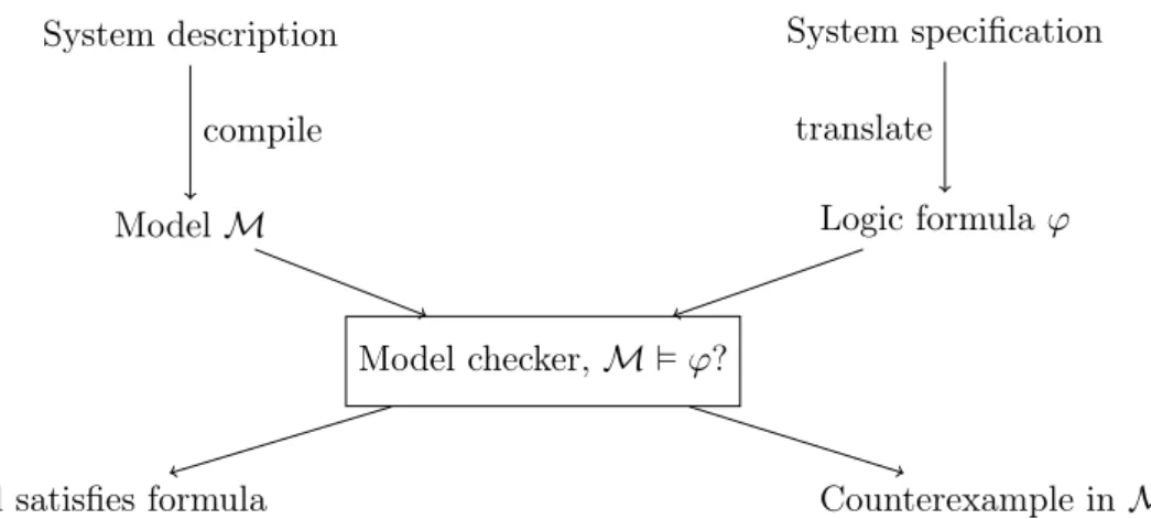
Figure 1.1: Model checking

like LTL or BTL, but the logic is usually tied to the expressiveness of the modelled system.

• Algorithms. These form the backbone of model checking as they are procedures for solving whether the model satisfies the specification.

The typical methodology for model checking involves each of the parts, its general concept is displayed in Figure 1.1. A system description (program) is compiled into the model M of the system, some kind of transition system, and the system specification is translated into a formula ϕ of the logic. Both are serve as input to the model checker, where a decision procedure concludes whether the model satisfies the formula (M ϕ) or not (M 6 ϕ). If M 6 ϕ, the model checker usually also yields a counterexample, witnessing the violation of the formula in the model.

Work in the branch of model checking focuses on two major parts. Finding new algorithms for existing models and specifications and showing their computational hardness or creating new models and specifications in order to model new kinds of programs or hardware.

The introduction of model checking offers some advantages over other methods

known. Firstly, the algorithmic nature of model checking. As such, model checking

can be automated and meets the goal to be integrated into the development process

of programs. Secondly, model checking can be used on very different systems, from

abstract modeling languages to hardware implementations. While each needs its

own model and specification language, the methodology stays the same across all

applications of model checking and knowledge can be spread across the fields. At

last, it can be used for checking concurrent programs, for which testing is not a

sufficient option due to the interaction of parallel processes. As an automated tool

designed to explore large state spaces, model checking is applicable for showing

correctness of concurrent programs.

correctness of a program, synthesis is about constructing a system that acts compliant with a specification. The motivation for synthesis is relief for the programmer from implementation details, increasing their focus on conceptual design. At the same time, synthesis entails a formal correctness proof for each generated program.

A typical setting for synthesis are “reactive systems”. Their specification consists of input and output parameters and they are generated such that the correct outputs for any inputs are produced. The synthesis problem motivates an extension to the model checking methodology by the use of games.

A typical model checking algorithm for a model M and a formula ϕ creates an automaton A

for the negated formula and builds the product model M × A

and runs an language emptiness test on it. If there is no accepting path in it, M satisfies ϕ. If there is an accepting path, it is a witness for a faulty behaviour. One could interpret these actions as a question “is there any input sequence such that M enters a faulty state?”. Naturally, the product automaton is a non-deterministic automaton where the environment of the program chooses the input parameters.

In the synthesis environment, this question needs to be adapted to “is there a model M that reacts to every input with the correct output, such that no input sequence brings M to a faulty state?”. Implicitly, this question brings a second kind of non-determinism into the synthesis problem. The first type of non-determinism is the environment, deciding the inputs as in typical model checking, the second one is the synthesizer, deciding the outputs with the ability to react to the input.

Formally, synthesis can be seen as a two player perfect information game and the task of finding a model M corresponds to finding a winning strategy in such a such game.

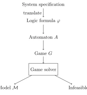
The concept of synthesis is displayed in Figure 1.2. A specification is translated into a formula ϕ, which is further translated into an automaton A. The automa- ton is then modified into a game G. Intuitivly, we split each transition of A into two halfs: the input transitions, which belong to the environment, and the output transitions, which belong to the synthesizer. If there is a winning strategy for the synthesizer, it outputs a model M that satisfies ϕ. Otherwise, there is no model for the specification. Synthesis based on this paradigm shares the positive properties of model checking. It can be automated and integrated into the development process.

However, the computational complexity of solving games on a model is usually a lot harder than the verification problem.

In this work, we focus on a model for concurrent, recursive programs: Multi- pushdown systems. Pushdowns can be used to model call stacks of recursive pro- grams, while a finite state space abstracts the set of (bounded) global variables.

In a concurrent world of recursive programs, each having their own call stack, the

adequate model also needs multiple pushdowns. As discussed earlier, only two push-

downs and a common finite state space are sufficient for most properties to become

undecidable. Various under-approximations have been suggested in order to arrive

at a decidable model, including bounded context switching and bounded phase com-

System specification Logic formula ϕ

Automaton A Game G Game solver

Model M Infeasible

translate

Figure 1.2: Program synthesis

putations [11, 14]. A context is part of a computation where only one pushdown is active, i.e. the system uses transitions acting on that stack only for the duration of the context. Similarly, a phase is part of a computation where only one pushdown uses pop transitions, i.e. the system uses any transitions execpt pop transitions.

These may only occur for the active pushdown during the phase. A multi-pushdown system with bounded context switching or bounded phase allows only computations that do not exceed a fixed number of contexts or phases.

The model checking problem for multi-pushdown systems with bounded context switching (phase) has been solved in EXPTIME (2-EXPTIME) [3], where the number k of contexts (phases) is part of the input. In this work, we focus on reachability and parity games on multi-pushdown systems with bounded context switching and phase, settling the complexity for game based synthesis and other proceedures looking to solve games on this model.

1996, Walukiewicz introduced the complexity of EXPTIME for single pushdown

games by creating a finite state game, exponential in the size of the pushdown sys-

tem [4, 16]. Key to the construction is to only remember the top of stack symbol of

the pushdown and maintain a prediction of possible popping scenarios. Whenever

a symbol would be pushed, one of the players proposes such a prediction P ⊆ Q

which is a subset of the states. The other player may either skip to one of the pro-

posed states or remember the set in the state. Whenever a symbol would be popped

from the pushdown, the winner of the play is determined depending on whether

P contained the popping scenario. The exponential size of the finite state game

is immediate, because the states space of the game consits of the whole powerset

of states. However, the construction could only determine the winner of positions

Seth adapted Walukiewicz’s approach in 2009 to find an algorithm solving bounded phase multi-pushdown games [13]. The construction contains a slight error, leading to missing winning strategies for the predicting player even though the original bounded phase multi-pushdown game was winning for them. We construct a very similar game to solve this problem for the bounded context switching case, resulting in a difference of two exponents in complexity to the bounded phase problem. In that work, Seth also suggests a non-elementary lower bound, encouraging further work in this direction.

Very recently, in 2017, there has been work in order to find a uniform solution for bounded phase multi-pushdown games as well [2]. The authors also mention an idea on how to show the non-elementary lower bound. In another publication [1], they find a non-elementary lower bound on model checking branching time logic for bounded context switching multi-pushdown systems by reducing from a Turing machine.

In this work, we settle a tight k-EXPTIME lower bound for k + 2 context bound multi-pushdown games and k phase bound multi-pushdown games. This confirms the non-elementary lower bound for both problems and tightens them for each fix bound on the contexts or phases. We use key elements of the construction in [1]

of bounded context switching and bounded phase multi-pushdown games such as the idea of storing a computation of the Turing machine on one stack, encoding the configurations of the Turing machine into a layered indexing system. We also use a kind of “Guess & Check” approach heavily for the correctness of the construction.

We also provide an upper bound of k-EXPTIME for k + 2 context bounded multi-

pushdown games. Together with Seth’s upper bound on the bounded phase case,

we can conclude k-EXPTIME completness for k + 2 context bounded and k phase

bounded multi-pushdown games.

First settle notation and definition of basic structures involved in multi-pushdown games. We define multi-pushdown systems, games, plays, winning conditions and games on multi-pushdown systems.

2.1 Multi-pushdown systems

A multi-pushdown system consists of a single state space, a finite number of stacks and a transition relation. Like a regular pushdown system, each transition pushes or pops a symbol on one of the stacks. Each stack is affected only by the transitions acting on them. A transition acting on one stack does not change the contents of any other stack.

Definition 1. A multi-pushdown system (mpds) P is a tuple (Q, Γ, δ, n) where Q is a finite set of states, n is the number of stacks, Γ is a finite alphabet and δ = δ

∪ δ

∪ δ

is a set of transition rules with

δ

⊆ Q × [1..n] × Q δ

⊆ Q × [1..n] × Γ × Q δ

⊆ Q × Γ × [1..n] × Q.

We denote the set of transition rules acting on stack r by

δ

= (δ

∩ (Q × {r} × Q)) ∪ (δ

∩ (Q × {r} × Γ × Q)) ∪ (δ

∩ (Q × Γ × {r} × Q)).

A configuration of P is of the form (q, S ) where q ∈ Q is the configuration’s state and S : [1..n] → Γ

⊥ are its stack contents. Each stack r is being assigned its content S

∈ Γ

⊥. The bottom of each stack consists of a non-removable symbol ⊥. We sometimes denote configurations of mpds with n stacks by (q, S

, . . . , S

). The top of the stack is on the left side in our notation.

The set of all configurations is C = Q × (Γ

⊥)

. We define the transition relation of the associated transition system.

Definition 2. The transition relation 7→ ⊆ C ×δ ×C implements the transition rules given by P on its configurations. For any two configurations, ((q, S), τ, (q

, S

)) ∈ 7→

if

• τ = (q, r, q

) ∈ δ

and S

= S

or

• τ = (q, r, s, q

) ∈ δ

and sS

= S

or

• τ = (q, s, r, q

) ∈ δ

and S

= sS

and for all stacks j 6= r, S

= S

.

We also denote this by (q, S) 7− →

(q

, S

). If the transition τ is of no importance, we may omit it. A computation of P is a sequence π = π

. . . π

∈ C

of configurations with π

7→ π

7→ · · · 7→ π

.

We restrict our computational model by introducing a bound to phases or contexts.

Definition 3. A context on stack r is a non-empty computation α = α

7−→

α

7−→

. . . 7−−→

α

such that each transition rule acts on stack r. I.e. for each position 0 ≤ p < l, τ

∈ δ

.

A phase on stack r is a non-empty computation α = α

7−→ α

7−→ . . . 7−−−→

α

such that each pop transition rule acts on stack r. Formally, there is a transition rule τ

∈ δ

∩ δ

and for each position 0 ≤ p < l, if τ

∈ δ

then τ

∈ δ

∩ δ

.

A computation π = π

7−→ π

7−→ . . . 7−−→

π

is a k context (phase) computation, if it consists of k contexts (phases):

α

= π

7−→ . . . 7−−−→

π

α

= π

τp1

7−−→ . . . 7−−−→

π

. . .

α

= π

7−−−→

. . . 7−−→

π

. Example 4. Let P = ({q

, . . . , q

}, {a, b}, δ, 2) where δ is given by the following figure. A transition

q push

a q

states the transition rule (q, 1, a, q

) and vice versa for popping transitions.

q

start q

q

q

q

q

push

a

pop

a push

b

pop

b pop

a

push

a

push

b

An example configuration of P is (q

, S) where S

= a⊥ and S

= ⊥, also denoted by (q

, a⊥, ⊥).

An example computation is

(q

, ⊥, ⊥) 7−−−−−−→

(q

, a⊥, ⊥) 7−−−−−−→

(q

, a⊥, b⊥) 7−−−−−−→

(q

, a⊥, ⊥) 7−−−−−−→

(q

, ⊥, ⊥) 7−−−−−−→

(q

, b⊥, ⊥) 7−−−−−−→

(q

, bb⊥, ⊥) . . .

which is a 3 context computation. It switches context at the transition (q

, 2, b, q

) and (q

, 1, a, q

) and then stays in context 3 forever.

When limiting contexts to 2 for example, the computation would stop in (q

, a⊥,

⊥) and no transitions could be used anymore.

2.2 Games

A game consists of a set of positions, a set of moves, two players, called Eve and Ana, and a winning condition. Each player owns a partition of the positions. They can play the game from some starting position and whenever the play is in a position owned by Eve or Ana respectivly, they choose a move from the set of moves to continue the play to the next position. When they complete a play, the winning condition decides the winner of that play.

Definition 5. A game is a tuple (V, E, W) together with an ownership function own : V → {Eve, Ana}, where V is a non-empty set of positions, E ⊆ V

is the set of moves and W : V

→ {Eve, Ana} is the winning condition.

Let ∈ {Eve, Ana} and V

= {v ∈ V | own(v) = }.

A play is a sequence π = (π

)

, such that for all p, π

π

∈ E.

A play π is winning for if W(π) = .

A strategy for is a function σ : V

V

→ V such that vσ(πv) ∈ E.

A strategy is positional, if σ : V

→ V .

A play π is compliant with strategy σ of if for all π

∈ V

: π

= σ(π

).

A strategy σ is called winning for from v ∈ V if all plays compliant with σ starting in v are won by .

There are a variety of different winning conditions. We focus on two winning conditions relevant in model checking: reachability and parity winning condition.

Definition 6. The reachability winning condition W

consists of a set of winning positions V

⊆ V and the winner of a play is determined by visiting a winning position:

W

(π) =

( Eve if there is π

with π

∈ V

Ana otherwise .

A reachability game is the tuple (V, E, V

).

The parity winning condition W

consists of a parity assignment Ω : V → [1..max]

and the winner of a play is determined by the greatest infinitly occuring parity during the play:

W

(π) =

( Eve if the greatest infinitly occuring parity in (Ω(π

))

is even

Ana otherwise .

A parity game is the tuple (V, E, Ω).

Even though plays are infinite by definition, we will allow games to contain posi- tions v that do not offer a move, i.e. E(v) = ∅ . A play ending in such a position v is losing for own(v) and thus winning for their opponent. There is a game equiv- alent to G, where we introduce the positions Evewin and Anawin with the moves ( win, win) and (v, win) if E(v) = ∅ and own(v) = 6= . We also complete the winning condition by

W

(π) =

( if win occurs in π

W(π) otherwise .

We use the term “ possesses a strategy from v to V

”, where V

⊆ V , as abbre- viation for: Player possesses a strategy σ, such that each play π compliant with σ starting in v visits a position π

∈ V

or is winning for player = W (π).

2.2.1 Game simulation

Later, we want to carry strategies from one reachability game to another. We intro- duce game simulation for reachability games in order to find those strategies without having to explicitly name them. Intuitivly, a game simulating another offers to re- produce moves from the original game. However, these do not have to be a single move. Instead we require a strategy for the owner of each state, that will bring them to the desired successing position.

Definition 7. A reachability game (V

, E

, V

) is simulated by (V

, E

, V

) if there is a function f : V

→ V

such that for each position v ∈ V

, with own(v) = and their opponent,

• own(v) = own(f (v))

• v ∈ V

if and only if f (v) ∈ V

• If v

∈ E

(v), then possesses a strategy σ

from f (v) to f (v

). Player possesses a strategy σ

from f(v) to f (E

(v))

• Let π = π

π

. . . be any play from f (v) compliant with σ

that contains a first position p with π

= f(v

). Then, for all 0 < u < p, π

6∈ V

• Let π = π

π

. . . be any play from f(v) compliant with σ

that contains a first position p with π

∈ f (E

(v)). Then, for all 0 < u < p, π

6∈ V

.

Lemma 8. Let A = (V

, E

, V

) be simulated by B = (V

, E

, V

) via f.

A position v ∈ V

is winning for Eve if and only if f(v) is winning for Eve.

Proof. Let possess a winning strategy σ

from a position v ∈ V

. We construct

a winning strategy σ

for from f(v). We construct this non-positional strategy

by remembering a play prefix π

π

. . . π

of A that is compliant with σ

. We show,

how σ

acts to continue a play prefix π

π

. . . π

in B , where ψ : N → N maps

positions in π to positions in π

such that

• for each u ∈ [0..i], f (π

) = π

• for each t ∈ [0..i − 1] and all ψ(t) < u < ψ(t + 1), π

6∈ V

.

Strategy σ

either wins the play π

from π

or continues to π

together with some π

, such that π

. . . π

π

is compliant with σ

. We construct σ

and show the correctness via induction:

Base Case (i = 0). π

= π

= v, ψ(0) = 0, π

= π

= f (v).

Inductive Case. Assume π

. . . π

is compliant with σ

and π

. . . π

is compliant with σ

and ψ is constructed according to the above invariant.

Case 1 (there is a position p, such that π

∈ V

): By induction, the play prefixes are according to the invariant. Thus, for each position 0 ≤ t < i, all ψ(t) < u <

ψ(t + 1) fulfill π

6∈ V

. The only position possible for p is p = ψ(t) for some 0 ≤ t ≤ i. By the invariant, f (π

) = π

= π

, and by definition of simulation π

∈ V

. Any play with the prefix π

. . . π

is winning for Eve. Since σ

was winning for and by induction, π

. . . π

is compliant with σ

, Eve = . Indeed, the winner of any play with prefix π

. . . π

is winning for Eve.

For the rest of the inductive case, assume that for all positions 0 ≤ p ≤ ψ(i), π

6∈ V

. In particular, the winning condition is independent of the play up to π

.

Case 2 (own(v) = ): Let v

= f(σ

(v)), Player continues the play by using strategy σ

, until

Case 2.1 (there occurs a first position p in π

, such that π

= f (v

)): Set ψ(i+1) = p.

Continue π

. . . π

by π

= v

. By definition of simulation and σ

, for all ψ(i) <

u < ψ(i + 1), π

6∈ V

.

Case 2.2 (f (v

) is not visited by π

): By definition, σ

is a strategy from f (v) to f(v

). Thus, any play compliant with that strategy that does not visit f (v

) is winning for .

Case 3 (own(v) = ): Player continues the play by using strategy σ

, until Case 3.1 (there occurs a first position p in π

, such that π

= f (v

), where v

∈ E

(v)):

Set ψ(i + 1) = p. Continue π

. . . π

to π

= v

. By definition of simulation and σ

, for all ψ(i) < u < ψ(i + 1), π

6∈ V

.

Case 3.2 (f (E

(v)) is not visited by π

): By definition, σ

is a strategy from f (v) to f(E

(v)). Thus, any play compliant with that strategy that does not visit f (E

(v)) is winning for .

Towards contradiction assume a play π

compliant with σ

is losing for . Then,

neither Case 1, Case 2.2 nor Case 3.2 happend during the play. Thus, π

is an infinite

play compliant with σ

and there is an infinite play π compliant with σ

together

with a function ψ according to the above conditions.

Case 1 ( = Eve): Since σ

is winning for Eve, there is a position π

∈ V

and thus π

= f (π

) ∈ f (V

) ⊆ V

, i.e. π

is winning for Eve.

Case 2 ( = Ana): Since σ

is winning for Ana, π does not visit V

and thus for all i ∈ N , π

6∈ V

. Furthermore, for all ψ(i) < u < ψ(i + 1), π

6∈ V

. Then, π

does not visit V

and the play is winning for Ana.

2.3 Multi-pushdown games

A multi-pushdown game is a game on the configurations of a multi-pushdown system.

The set of positions is the set of configurations of the multi-pushdown system and the set of moves is the transition relation. Ownership is determined by partition of the state space of the multi-pushdown system.

Definition 9. Let P = (Q, Γ, δ, n) be a multi-pushdown system.

A multi-pushdown game (mpdg) (P, W ) is the game (C, 7→, W ) with ownership func- tion own : Q → {Eve, Ana} that carries over to positions of the game via own(q, S) = own(q).

For the winning condition, we consider state reachability games, configuration reachability games and parity games.

Definition 10. The configuration reachability mpdg (P, C

) with winning region C

⊆ C is the reachability game (C, 7→, C

).

The state reachability mpdg (P, Q

) with winning states Q

⊆ Q is the con- figuration reachability mpdg (P, Q

× (Γ

)

).

The parity mpdg (P, Ω) with parity assignment Ω : Q → [1..max] is the par- ity game (C, 7→, W

) where the parity assignment carries over to positions via Ω(q, S ) = Ω(q).

As a stronger computational model than multi-pushdown systems, multi-pushdown games are also Turing complete. We apply the previous restrictions for multi- pushdown systems.

Definition 11. A k-context (phase) bounded multi-pushdown game (P, W , k) is a variation of the mpdg (P, W) where no play may exceed the k’th context (phase).

Moves that would introduce a k + 1’th context (phase) do not exist.

We omit a more formal definition for the sake of notation. It should be noted

that this way some plays may not be continued at all. There are different ways to

approach this. We choose that the player owning the position, from which the play

can not be continued, looses the game. The lower bound construction is unaffected

by this, as the mpdg constructed there will stay within k contexts (phases) for any

computation and will always offer a possible transition. For the upper bound, we

assume that there will always be a possible transition from each position without introducing a k + 1’th context. An equivalent mpdg with this condition can be constructed analoge to the construction in section 2.2 about games in general.

Example 12. We use the multi-pushdown system from example 4 for an exam- ple multi-pushdown game. We add the ownership function own : {q

, . . . , q

} → {Eve, Ana} by shaping the states in the mpds graph. A round state belongs to Eve and a rectangle one to Ana. We also set a parity function Ω : {q

, . . . , q

} → {0, 1}

by writing the parities at the bottom of each state.

q

start

q

q

q

q

q

1 0

0

1 1 0

push

a

pop

a push

b

pop

b pop

a

push

a

push

b

Since the parities Ω(q

) = Ω(q

) = 0 are winning for Eve, each play is winning for Eve in this multi-pushdown game.

If we limit the amount of contexts to 2 however, Ana gains a winning strategy, by taking using the transition rule (q

, 2, b, q

). The play continues to the configuration (q

, a⊥, ⊥). As in example 4, the number of contexts can not be further increased and Eve, who owns q

, has no transitions they can take which causes them to loose the play.

For better construction of mpdg, we introduce push and pop transitions of regular expressions instead of single symbols. Each such transition is a short notion for a set of transitions, that allow the player owning the state to push or pop any word matching the regular expression.

Definition 13. Let R be a regular expression and (Q

, δ

, I

, F

) be the NFA accepting R.

We write the transition rules

(q, r, R, q

) for pushing a word belonging to R onto stack r (q, R, r, q

) for popping a word belonging to R from stack r as a replacement for a finite number of transition rules.

A pushing transition rule (q, r, R, q

) is replaced by finitly many transition rules:

q q

q

q

q

q

for each q

∈ I

for each (q

, s, q

) ∈ δ

for each q

∈ F

int

push

s

int

We also set the ownership of all q

∈ Q

to own(q

) = own(q).

Analogously for a popping transition rule, except that we pop instead of pushing:

q

pop

s q

for each (q

, s, q

) ∈ δ

.

However, this construction has a flaw. In a reachability mpdg, a pushing transition of the above form may allow Ana to loop in an infinite cycle within the NFA and not ever complete the transition. This would result in a winning play for them. Popping transitions do not suffer this problem as the stack height is finite. We circumvent this problem by only using regular expressions that do not contain kleene iteration or complement when giving Ana a regular expression pushing transition, as there are NFA without cycles to accept them.

Example 14. The regular expression {a, b}

has the NFA q

start a, b

A pushing transition (q, r, {a, b}

, q

) is replaced by the transitions

q int

q

q

push

a, b int

In a reachability game, Ana can loop forever in q

which might form a winning

strategy for them, as no other state would ever be visited.

In this section, we present a finite game that is equivalent to a context bounded multi-pushdown game. The size of the finite game depends on the number of contexts allowed.

Theorem 15. k + 2-context bounded multi-pushdown parity games can be solved in k-EXPTIME.

For the rest of the section, let G

= (P, Ω, k) be a k-context bound multi-pushdown game with P = (Q, Γ, δ, n), Ω : Q → [0..max] and own : Q → {Eve, Ana}. The game G

consists of infinitly many positions: The set of configurations of P is infinite, because the stack contents can grow arbitrarily large. The goal is to reduce this amount of positions to a finite number. Intuitivly, we forget the exact stack contents and only remember the top of stack symbol for each stack. This idea is similar to Walukiewicz’s construction [16]. In fact it is a variation of Anil Seth’s construction for bounded phase multi-pushdown games, which contains a slight constructional error. We will see an example for which Eve fails to obtain a winning strategy in Seth’s finite game, even though they possess a winning strategy in the original mpdg.

Remembering only the top of stack symbol for each stack makes it impossible to continue a play that used a pop transition, since the next top of stack symbol was forgotten. To circumvent this problem, we use a Guess & Check approach that ends any play when it discovers its first pop transition. Whenever a symbol is pushed on one of the stacks, Eve suggests a set of popping scenarios for this symbol. The idea is that Eve can fix their strategy and they can predict all plays compliant with this strategy. They can collect all situations where eventually the pushed symbol is popped and create the desired set of popping scenarios. We call this set a prediction set. Given a prediction set, Ana has two choices. They can choose one of the popping scenarios given in the prediciton set and move to its corresponding position, skipping the play in between. Or they actually perform the pushing transition. In the second case, we remember the prediction set in the positions of the finite game. This is necessary to determine a winner, when a popping transition is used. Whenever a popping transition is used, the game looks up whether the remembered prediction set contains the current situation as a popping scenario and determines the winner of the play.

3.1 Push-pop-pairs, stairs and notation

We first settle some notation and define push-pop-pairs, last unmatched pushes and

stairs. Remember that a play of G

is a computation (q

, S

) 7−→

(q

, S

) 7−→

. . .

where each q is a state and each S is a function assigning each stack its contents.

In the rest of the section occur many functions of the form T : [1..n] → A assigning each stack some information.

Definition 16. Let T : [1..n] → A for some set A. For each r ∈ [1..n] and x ∈ A, we use the notation T

for T (j) and T [x/r] which replaces the information for stack r by x:

T [x/r]

=

( x j = r T

otherwise.

A push-pop-pair of a play for an mpdg are two positions. The first position is a pushing transition and the second is the popping transition that pops precisly the symbol pushed by the push transition.

Definition 17. A push-pop-pair of a play (q

, S

) 7−→

(q

, S

) 7−→

. . . of G

are two indices (p, p

) ∈ N

such that there is a stack r with

• p < p

• τ

∈ δ

∩ δ

• τ

∈ δ

∩ δ

• min{|S

|, . . . , |S

|} > |S

| = |S

|

Note that each p ∈ N is in at most one push-pop-pair.

Definition 18. Let π = π

7−→

π

. . . be a play of G

. We call a pushing position p ∈ N with τ

∈ δ

matched, if there is p

∈ N such that (p, p

) is a push-pop-pair.

Otherwise, the push is unmatched.

For each stack j, we define the function lup

: N → N which finds the last un- matched push of stack j in π.

lup

(p) = max

0≤u<p τu∈δ_push

{u | u unmatched in π

. . . π

}

Be aware, that if no such pushing position exists, lup

(p) = ⊥ is undefined.

Definition 19. Let π be a play and p ∈ N . Let π

= (q

, S

).

A stair p ∈ N of π is a position where for all i ∈ N with p ≤ i and each stack j ∈ [1..n], |S

| ≤ |S

|.

Be aware, that by this definition there is no push-pop-pair (p

, p

) such that p

<

p < p

.

3.2 Finite state game

We construct the finite state game FSG equivalent to the multi-pushdown game G

. It consists of positions of the form

(Check, q, c, d, γ, P , m).

They represent positions of G

with additional information. The positions contain

• q, the state of the configuration.

• c, the context of the computation.

• d, the stack holding the current context.

• γ : [1..n] → Γ, the current top of stack symbols.

• P : [1..n] → P , a prediction set for each stack. This is explained later.

• m : [1..n] → [1..max], the maximal parity seen for each stack since the the last unmatched push of that stack.

We will define a set of predictions P . Each element of P describes a popping scenario. We partition the set in smaller sets P = ∪

P

. An element of P

describes a situation where the top of stack symbol from stack r is popped during context j.

Intuitivly, when a player wants to use a pushing transition for stack r, instead Eve will guess a set P

⊆ ∪

P

. After Eve suggests such a prediction set, Ana may either choose a popping scenario from the set and skip the computation in between, or actually perform the pushing transition. In this case, either the pushed symbol is never popped, or when it is popped, one of the players is determined as winner of this play by the use of the current prediction sets P .

A popping scenario contains more than just the top of stack symbols, the state and the context after popping. It also contains the maximal parity for each stack since their last unmatched push and a prediction set for each stack.

Such a popping scenario can be thought of as an abstraction of the computation from the pushing position up to the popping position. Other stacks can have pushed or popped symbols in the mean time, creating different prediction sets for them. A popping scenario thus also contains a prediction set for each other stack.

Definition 20. Let q, γ, m range over Q, Γ

, [1..max]

. For each r ∈ [1..n], j ∈

[3..k − 1] define the prediciton sets

P

= {(P

, . . . , P

, (q, k, γ, m), P

, . . . , P

) | P

= · · · = P

= ∅ } P

= {(P

, . . . , P

, (q, 1, γ, m), P

, . . . , P

) | P

= · · · = P

= ∅ } P

= {(P

, . . . , P

, (q, 2, γ, m), P

, . . . , P

) | P

= · · · = P

= ∅ } P

= {(P

, . . . , P

, (q, c, γ, m), P

, . . . , P

)

| P

⊆ ∪

P

, . . . , P

⊆ ∪

P

} for 3 ≤ c < k

P

=

k

[

c=1

P

An element of P ∈ P

describes a situation where the topmost symbol from stack r is popped in context c. It contains the tuple (q, c, γ, m), containting information of the configuration after popping:

• q the state

• c the context

• γ the top of stack symbols

• m the maximal parity seen for each top of stack symbol since its respective push operation.

It also contains P

, . . . , P

, P

, . . . , P

, a guarantee for the prediction sets that were created during computation up to this popping scenario for each top of stack symbol. We call them a guarantee, because the prediction set for another stack j at the popping position may actually contain more popping scenarios than P

. That prediction set was made before the popping scenario P happened. Thus, there might be popping scenarios for that top of stack symbol that don’t include P in their play.

Example 21. Recall example 12. We used the following multi-pushdown game.

q

q

q

q

q

q

1 0

0

1 1 0

push

a

pop

a push

b

pop

b pop

a

push

a

push

b

Assume a play in configuration (q

, ⊥, ⊥) in a context c > 2 on stack 1 (We want the context to be greater than 2 for demonstration purposes). The next transition (q

, 1, a, q

) is a pushing transition. In the corresponding FSG, Eve has to push a prediction set. They do not know whether Ana wants to continue the play to either q

or q

. Eve has to collect all possible popping scenarios for the symbol that is being pushed. Looking at the transitions, it is immediate that there are precisly two popping scenarios. One is the transition (q

, a, 1, q

) and the other transition is (q

, a, 1, q

) for another play.

Eve then proposes a prediction set P with two elements P

and P

where they include the correct parameters for

P

= (q

, c, (⊥, ⊥), (0, 0)) P

= (q

, c + 2, (⊥, ⊥), (1, 1)).

As discussed, Eve also has to propose guarantees for the prediction sets for stack 2 in each scenario. Since in both scenarios, the top of stack symbol of stack 2 is ⊥ which is never popped, the sets P

= P

= ∅ are empty.

Assume Ana decides not to skip to one of the predicted scenarios. Instead, we remember P for stack 1 and the game continues in q

. Let Ana choose the transition (q

, 2, b, q

). Eve has to make a new prediction, this time for stack 2. There is only one popping scenario P

for this symbol:

P

= (q

, c + 1, (a⊥, ⊥), (1, 1))

and the prediction guarantee for the current stack 1 top of stack symbol. Note that Eve now knows more precisly about the possible popping scenarios of the pushed a.

They can reduce the prediction set for that stack by setting P

= {P

}.

Be aware that they cannot even add the prediction P

to this set: Since P

∈ P

is a scenario for popping in context c + 1 and P

∈ P

is a scenario for popping in context c, the construction does not allow that scenario as a guarantee (see Definition 20).

Assume Ana again does not skip to the proposed popping scenario but remembers

the prediction set {P} for stack 2. Note that the remembered prediciton set for stack

1 is still P = {P

, P

}. The next transition is a popping transition (q

, b, 2, q

) and

the finite state game is supposed to find a winner for the play. It will see that the

prediction set for stack 2 is {P}. The context, the resulting state after popping,

the top of stack symbols and the maximal parities seen for each stack are correct

in P . Also, the given guarantee P

for stack 1 is fitting. The current remembered

prediction is still P = {P

, P

} ⊇ {P

} = P

. In other words, it contained the

popping scenarios which were guaranteed to exist by the popping scenario P

.

3.2.1 Construction

We construct the finite state game for G

. For a position (Check, q, c, d, γ, P , m), and a stack r, define

c

=

( c d = r c + 1 d 6= r . The following moves are only introduced, if c

≤ k.

1. (q, r, q

) ∈ δ

:

(Check, q, c, d, γ, P , m) → (Check, q

, c

, d

, γ, P , m

) where a) m

= max{m

, Ω(q

)} for each 1 ≤ j ≤ n

b) d

= r

2. (q, r, s, q

) ∈ δ

:

a) (Check, q, c, d, γ, P , m) → (Push

, c

, γ, P , m, q

, s)

b) (Push

, c

, γ, P , m, q

, s) → (Claim

, c

, γ, P, m, q

, s, P) where P ⊆ P

. c) (Claim

, c

, γ, P , m, q

, s, P ) → (Check, q

, c

, r, γ[s/r], P [P/r], m

) where

for each stack j 6= r, m

= max{m

, Ω(q

)} and m

= Ω(q

).

d) • (Claim

, c

, γ, P, m, q

, s, P) → (Jump

, q

, c

, γ

[γ

/r], P

, m

, m

) for each P

∈ P, where P

= (q

, c

, γ

, m

) with c

6= 2 and P

= P

[P

/r].

• (Claim

, c

, γ, P, m, q

, s, P) → (Jump

, q

, c

, γ

[γ

/r], P, m

, m

) for each P

∈ P where P

= (q

, 2, γ

, m

).

e) (Jump

, q, c

, γ

, P

, m

, m

) → (Check, q

, c

, r, γ, P

, m

) where m

=

( max{Ω(q), t

, m

} j = r max{Ω(q), t

} j 6= r

3. (q, s, r, q

) ∈ δ

:

• (Check, q, c, d, γ[s/r], P, m) → Evewin if P

∈ P

• (Check, q, c, d, γ[s/r], P, m) → Anawin if P

6∈ P

where

P

= ∅ [(q

, c

, γ, m)/r] if c

= k or c

= 2

P

⊆ P

, P

= (q

, c

, γ, m) for all j 6= r, if 2 6= c

< k

Together with the parity assignment

Ω

((Check, q, c, d, γ, P , m)) = Ω(q) Ω

((Push

, . . . )) = Ω

((Claim

, . . . )) = 0

Ω

((Jump

, q, c

, γ

, P

, m

, m

)) = m

Ω

(Evewin) = 0 Ω

(Anawin) = 1 this defines a parity game FSG = (V

, E

, Ω

).

Constructional error in Seth’s construction Seth’s construction [13] is very similar to the above one. However, in the transitions introduced for popping a symbol and determining a winner of the play, the guarantees had to equal the current prediction in the position, i.e. given a transition rule (q, s, r, q

) ∈ δ

, the following moves were introduced

• (Check, q, c, d, γ[s/r], P , m) → Evewin if P

∈ P

• (Check, q, c, d, γ[s/r], P , m) → Anawin if P

6∈ P

where

P

= ∅ [(q

, c

, γ, m)/r] if c

= k or c

= 2 P

= P

, P

= (q

, c

, γ, m) for all j 6= r, if 2 6= c

< k

The constructional difference is P

= P

instead of P

⊆ P

. In example 21, we can see that Eve has no way to achieve this equality in that particular multi-pushdown game. Even though Eve possesses a winning strategy in the multi-pushdown game (See example 12), Ana would possess a winning strategy in the resulting finite state game.

3.2.2 Strategy automaton

To transport a strategy σ of FSG to G

, we introduce a strategy automaton S

. Intuitivly, this is an multi-pushdown system with the same number of stacks as P.

At any point in the game, the stack heights of S

are identical to the stack heights of P . However, we will not use the transitions of a common mpds. Instead, each transition will change all the top of each stack at once. Also, the stack alphabet of S

is Γ × 2

× [1..max] and has another state space.

The strategy automaton remembers information of the finite state game in the

following sense. If the finite state game would be in a position (Check, q, c, d, γ, P, m),

then the strategy automaton is in state (q, c, d) and the top of stack tuple of each

stack r is (γ

, P

, m

). At the same time, it mimics moves of G

. The automaton

can use the additional stack information to choose the next move by using σ from

the position (Check, q, c, d, γ, P , m) if it belongs to Eve. Otherwise, it just mimics the move made by Ana. Below is listed, how S

updates upon a move in G

. This is independent to whichever player makes the move. Be aware, that the configuration of S

can be used to derive a move for Eve, when they possess a strategy in FSG.

Definition 22. Given a strategy σ for Eve in FSG, the strategy automaton S

is a tuple S

= (Q × [0..k] × [0..n], Γ × 2

× [1..max], 7→, n) where

• Q × [0..k] × [0..n] is the state space,

• Γ × 2

× [1..max] is the stack alphabet and

• 7→ is a transition relation, that is defined on the set of configurations.

A configuration of S

is ((q, c, d), R), where R : [1..n] → (Γ × 2

× [1..max])

are the stack contents. For each stack j,

R

=

R

|R_j|^j

R

|R_j|−1

. . .

R

, where

R

|Rj|

is the top of stack symbol. Since each stack symbol

R

is a tuple, we denote them by

R

= (

γ

,

P

, m

).

For the sake of notation, we introduce a context sensitive top of stack pointer ↑.

It obtains the index value of the top of stack symbol:

R

=

R

|Rj|^j

R

|Rj|−1

. . .

R

=

R

R

. . .

R

.

This notation also carries over to the individual tuple contents. Thus,

j

γ

↑

=

γ

|Rj| ^j

P

=

P

|Rj| ^j

m

=

m

|Rj|

. We call the set of all configurations C

.

Definition 23. We define a function F : C

→ V

mapping configurations of S

to positions in FSG.

F (((q, c, d), R)) = (Check, q, c, d, γ, P , m) where γ

=

γ

, P

=

P

and m

=

m

.

Definition 24. We define the transition relation ((q, c, d), R) 7− →

((q

, c

, r), R

), where

c

=

( c d = r

c + 1 d 6= r and γ

=

γ

.

Let F (((q, c, d), R)) = (Check, q, c, d, γ, P , m). A transition is only introduced, if

c

≤ k and one of the following is true.

1. τ = (q, r, q

) ∈ δ

and each of the following

a) own(q) = Ana or σ((Check, q, c, d, γ, P , m)) = (Check, q

, c

, r, γ, P , m

) b) R = R

, except

• for each stack j,

m

= max{Ω(q

), m

}.

2. τ = (q, r, s, q

) ∈ δ

and each of the following

a) own(q) = Ana or σ((Check, q, c, d, γ, P , m)) = (Push

, c

, γ, P , m, q

, s) b) R = R

, except

• for each stack j 6= r,

m

= max{Ω(q

), m

},

• R

= (s, P , Ω(q

))R

, where

σ((Push

, c

, γ, P , m, q

, s)) = (Claim

, c

, γ, P, m, q

, s, P).

3. τ = (q, s, r, q

) ∈ δ

and each of the following

a) own(q) = Ana or σ((Check, q, c, d, γ, P , m)) = Evewin

b) there is P ∈ P

with P

= (q

, c

, γ

, m) such that for each stack j 6= r,

• c

6= 2 and P

⊆ P

or

• c

= 2 and P

= ∅ c) R = R

, except

• for each j 6= r,

–

m

= max{Ω(q

), m

}

–

P

=

( P

c

6= 2

j

P

↑

c

= 2

• R

= (

γ

,

P

, m

)

R

R

. . .

R

where

m

= max{

m

, m

, Ω(q

)}.

4. τ = (q, s, r, q

) ∈ δ

and each of the following

a) own(q) = Ana or σ((Check, q, c, d, γ, P , m)) = Anawin

b) there is no P ∈ P

with P

= (q

, c

, γ

, m) such that for each stack j 6= r,

• c

6= 2 and P

⊆ P

or

• c

= 2 and P

= ∅ c) R = R

, except

• for each j 6= r,

m

= max{Ω(q

), m

}