Nernst eect of Ni-doped NdBa2

Inaugural Dissertation

zur

Erlangung des Doktorgrades

der mathematisch-naturwissenschaftlichen Fakultat der Universitat zu Koln

vorgelegt von

Niko Johannsen

aus Mainz

Koln, im Mai 2008

Vorsitzender

der Prufungskommission: Prof. Dr. U. Ruschewitz

Tag der mundlichen Prufung: 26.6.2008

Es rauszunden ist die Picht, Die uns das Schicksal zugemi ß t.

Nein: zugemu ß t. Nein: zugema ß t.

Ich wei ß es nicht.

Wei ß t Du es denn?

Robert Gernhardt

1 Introduction 1

2 Formal Transport Theory 5

2.1 Basic equations . . . . 5

2.1.1 Electric conductivity in a magnetic eld . . . . 6

2.1.2 Heat conductivity in a magnetic eld . . . . 6

2.2 Galvanomagnetic eects . . . . 6

2.2.1 Isothermal test conditions . . . . 7

2.2.2 Adiabatic test conditions . . . . 7

2.3 Thermomagnetic eects . . . . 7

2.3.1 Isothermal test conditions . . . . 8

2.3.2 Adiabatic test conditions . . . . 8

2.3.3 Relations between transport coecients . . . . 9

2.3.4 Notations . . . . 9

3 Introducing the Seebeck and Nernst Eects 11 3.1 Seebeck eect . . . . 11

3.2 Nernst eect . . . . 14

3.2.1 Finite magnetic eld . . . . 14

3.3 Some examples . . . . 16

3.3.1 Bismuth . . . . 16

3.3.2 NbSe 2 . . . . 17

3.3.3 URu 2 Si 2 . . . . 18

3.3.4 CeCoIn 5 . . . . 19

3.3.5 Ferromagnetic materials . . . . 20

3.4 Nernst eect in the vortex liquid phase . . . . 21

4 Superconductivity 23 4.1 Introduction . . . . 23

4.1.1 Theoretical background . . . . 23

4.1.2 Pinned and depinned vortices . . . . 27

4.2 Vortex dynamics . . . . 30

4.2.1 Voltages in high-T c materials . . . . 30

4.2.2 Some forces on vortices . . . . 31

4.2.3 Vortex motion in a transport current . . . . 32

4.2.4 Spectral ow . . . . 35

4.2.5 Vortex motion in a temperature gradient . . . . 41

4.2.6 Summary . . . . 43

4.3 The system NdBa 2 {Cu 1-y Ni y } 3 O 7 − δ . . . . 44

4.3.1 Structure . . . . 44

4.3.2 Doping . . . . 46

4.4 Pseudogap - a brief overview . . . . 50

5 Experimental 53 5.1 Measurement of transport properties . . . . 53

5.1.1 Preparing electrical contacts . . . . 53

5.1.2 Stabilizing temperature and magnetic eld . . . . 56

5.1.3 Sweeping the eld or the temperature . . . . 57

5.2 Data analysis . . . . 59

5.2.1 Extracting the Nernst signal . . . . 59

5.2.2 Sign conventions . . . . 61

5.2.3 Error analysis . . . . 61

5.2.4 Nernst eect calibration in La 2−x Sr x CuO 4 . . . . 63

6 Motivation 67 7 Nernst Eect and Transport in Ni-doped NdBa 2 Cu 3 O 7−δ 73 7.1 Thermal conductivity . . . . 74

7.1.1 Introduction . . . . 74

7.1.2 Data and analysis . . . . 75

7.2 Seebeck eect . . . . 80

7.2.1 Introduction . . . . 80

7.2.2 Data and analysis . . . . 80

7.3 Nernst eect . . . . 87

7.3.1 Data and analysis . . . . 87

7.3.2 Phasediagram, conclusion and outlook . . . . 91

7.4 Thermal Hall angle . . . . 96

8 Nernst Eect and Transport in UPt 2 Si 2 101 8.1 Motivation . . . 101

8.2 Physical background . . . 101

8.3 Magnetic properties and structure of UPt 2 Si 2 . . . 103

8.4 Measurements and analysis . . . 103

8.4.1 Conguration (∇T, j) k a , B k c . . . 104

8.4.2 Conguration ∇T k c , B k a . . . 113

8.4.3 Conclusion . . . 116

9 Summary 117

List of Figures 123

Bibliography 125

Publications 137

Danksagung 139

Ozielle Erklarung 141

Abstract 143

Kurzzusammenfassung 145

Since the discovery of high-temperature superconductivity by Bednorz and Muller more than 20 years ago [1], the search for its mechanism is enthusiastically carried on. Still driven by the dream of superconductivity at room temperature, many promising experiments are performed in this special class of ceramic superconductors. It is known that magnetic elds can enter into these systems in units of elementary ux quanta. Such a ux line is encircled by a supercurrent of Cooper-pairs [2]. The whole entity is referred to as vortex. These structures can be forced to move through the sample by either applying a temperature gradient or a transport current. A moving vortex produces a voltage which is directed per- pendicular to its moving direction. This is due to quantum-mechanically induced phase- slips. When vortices move down the temperature gradient a voltage perpendicular to ∇T is detected. This is the Nernst eect. Introduced by Nernst and Ettingshausen in 1886 [3], this eect was long time left unnoticed, mainly because it is vanishingly small in normal metals. Nowadays, the impact of this eect truly justies calling it a renaissance of the Nernst eect. This is because it turned out that the transverse voltage in the vortex liquid phase causes an extraordinary large anomalous Nernst eect that is highly non-linear in its magnetic eld dependence. These ndings immediately identied the Nernst eect as one of the most sensitive tools for the detection of the motion of vortices or vortex-like excitations. In 2000 [4], Xu et al. published the nding of large Nernst signals lasting to temperatures far above the critical temperature ( T _c ) in La _2-x Sr _x CuO ₄ . The interpretation was straightforward: Since vortices are unambiguously related to superconductivity, there has to be at least some fraction of superconducting densities above T _c . Depending on the charge carrier concentration, T _c forms a superconducting dome in the cuprates. If we now leave the superconducting dome on the underdoped side by increasing the temperature above T _c , it turns out that the system is still far from behaving like a normal metal. Up to temperatures as high as room temperature there is a so-called pseudogap phase. Pseudo refers to the fact the density of states is only reduced rather than zeroed, as in a normal gap. This observation was based on data of optical conductivity measurements [5]. The nature of this phase is discussed in terms of an onset of a spin-pairing mechanism, sim- ilar to the Cooper-pair formation at T _c [68]. It seems to be a good approach towards the understanding of the mechanisms of high-T c superconductivity to rst understand the normal state from which it arises.

Here, the Nernst eect comes back into play. Its sensitivity in detecting signatures

of the superconducting state can be exploited to unravel possible relations between the

pseudogap and superconductivity. As a function of charge carrier doping in the cuprates,

T _c is found to increase until a maximum value is reached while the pseudogap temperature

T ^∗ decreases. By determining the onset temperatures of the anomalous Nernst signal in

this doping range, it is very interesting to observe whether it shows some scaling behavior with either one of the two phases. Such measurements were carried out by Wang et al. [9], obtaining onset temperatures that were interpreted as tracking T ^∗ .

In order to further investigate this aspect, it would be very helpful to examine a sys- tem in which the most relevant parameters, T _c and T ^∗ , can be tuned individually. Given such a system, one could examine whether there is a relation between the pseudogap and superconductivity by shifting the pseudogap and observing if the Nernst signal follows or not. Fortunately, such a system exists, namely NdBa 2 {Cu 1−y Ni y } 3 O 7−δ . Recent measure- ments of the optical conductivity of Ni-doped NdBa 2 Cu 3 O 7−δ revealed a strongly enhanced pseudogap while superconductivity is suppressed at the same time [10]. This compound therefore oers the unique opportunity to study the development of the Nernst signal while tuning T _c and the pseudogap individually and even in opposite directions. This is the sys- tematic investigation that is presented in this work. The measurements were performed on a series of optimally doped (O 7 ) and two series of underdoped (O 6.8 and O 6.9 ) samples with Ni contents ranging from y = 0 to 0.12. These data as well as a detailed analysis of their scaling relations with either T _c or T ^∗ represent the heart of this thesis.

The second part of this work leaves the physics of the high-T c 's, but still deals with the Nernst eect. After extensive studies of the Nernst eect in the high-T c 's, it was also studied in some superconductors with low T _c 's. Among them were samples of the class of the heavy Fermions. There it turned out that large Nernst eects are also present in other phases but the superconducting one. As an example, in URu 2 Si 2 , which is superconducting below 1.5 K, a Nernst signal could be resolved below 17.5 K [11]. This temperature marks the onset of a mysterious phase referred to as hidden-order phase. Consequently, new mechanisms had to be discussed as sources of an enhanced Nernst signal in such systems.

These mechanisms are searched for quite similar to the analysis of the physics of the thermopower by means of the Mott formula. An altered Mott formula for the Nernst eect suggests that a large Nernst signal can be caused by small Fermi energies and long scattering times, in some simple cases. These conditions can be met in very clean systems with low itinerant charge carrier densities. The ndings of a large Nernst eect that emerges with the onset of the mysterious hidden-order in URu 2 Si 2 impelled the investigation of the Nernst eect in the related system UPt 2 Si 2 in this work. UPt 2 Si 2 is a system that is neither superconducting nor is it a heavy Fermion. It is a local moment antiferromagnet with an ordering temperature of ' 31 K [12]. The more surprising that a pronounced Nernst eect is found to emerge with the antiferromagnetic ordering. Not only the Nernst signal, but a detailed analysis of all participating transport properties has been performed in this work.

Additional measurements of the Seebeck and Hall eects, the magnetoresistivity and the

thermal Hall eect, also referred to as Righi-Leduc eect, are shown. An early theory,

published in 1972 [13, 14], calculated the thermopower and the Nernst eect for generic

antiferromagnets. Included in the calculations is the appearance of a charge gap at the

Fermi surface upon entering into the antiferromagnetic order. This gap, together with a

modeling of spin and phonon scattering mechanisms leads to a substantial increase of the

thermomagnetic quantities according to the predictions of the theory. The measurements

on UPt 2 Si 2 and a detailed comparison to the results of this theory are shown in the second

and adiabatic test conditions. In chapter 3, the Nernst eect is discussed in more detail.

By some examples of recent studies, dierent mechanisms that are proposed to eect large

Nernst signals are illustrated. Chapter 4 briey introduces the theory of superconductivity

with emphasis on properties of the high-T c 's that is needed to become familiar with the

vocabulary used later on. It further illustrates how vortices produce voltages in situations

of applied transport currents and temperature gradients. Chapter 5 describes in detail the

experimental subtleties of this work. Chapter 6 gives a detailed motivation for the inves-

tigation of this work. Finally the measurements and the detailed analysis are presented in

chapter 7. The investigation of transport properties of UPt 2 Si 2 is completely covered in

chapter 8 and the main results are summarized in chapter 9.

2.1 Basic equations

In this chapter a brief overview into the basic theory of transport phenomena will be given. First the general denitions of the transport coecients will be introduced as they are derived from statistical mechanics. Then some special cases are discussed as the main focus of this thesis lies in measurements of the Nernst eect, the thermopower or Seebeck eect and the thermal conductivity. A detailed derivation of the transport equations is given in refs. [1522]. The tensor equations for the charge and heat current densities are:

j = L 11 E + L 12 (−∇ T) and (2.1)

j _h = L ₂₁ E + L ₂₂ (−∇ T). (2.2)

Solving these equations for the heat current density j _h and the electric eld E , we get

E = ρj + S∇ T and (2.3)

j _h = Πj − κ∇ T. (2.4)

The coecients used above are dened by

Electrical resistivity tensor: ρ = (L ₁₁ ) ⁻¹ , (2.5) Seebeck tensor: S = (L ₁₁ ) ⁻¹ · L ₁₂ , (2.6) Peltier tensor: Π = L ₂₁ · (L ₁₁ ) ⁻¹ , (2.7) Heat conductivity tensor: κ = L ₂₂ − L ₂₁ · (L ₁₁ ) ⁻¹ · L ₁₂ . (2.8) In the presence of a magnetic eld, the tensor coecients in equations (2.1) and (2.2) fulll the symmetries that depend on the magnetic eld according to the universal Onsager relations,

L 11 (B) = L 11 T (−B), L 22 (B) = L 22 T (−B), L 12 (B) = L 21 T (−B). (2.9) and thereby

ρ _ij (B) = ρ _ji (−B), κ _ij (B) = κ _ji (−B), S _ij (B) = S _ji (−B), Π _ij (B) = Π _ji (−B).

(2.10)

2.1.1 Electric conductivity in a magnetic eld

All external sources such as electric currents or temperature gradients are dened to be applied in x direction as not mentioned otherwise. If a magnetic eld is applied to the sample it will be in z direction. So the transverse eects will be monitored in y direction.

For the electrical conductivity under the inuence of a magnetic eld, Eq. (2.3) becomes E _x =ρ _xx (B) · j _x + ρ _xy (B) · j _y and (2.11) E _y =ρ _yx (B ) · j _x + ρ _yy (B) · j _y , (2.12) which resembles the ohmic law. The symmetric part of the resistivity tensor can be written as

ρ xx (B) = 1

2 ρ(B) + ρ(−B )

. (2.13)

The symmetry can be deduced from Eq. (2.10),

ρ _xx (−B ) = ρ _xx (B) (2.14)

and means that all elements of the symmetric conductivity tensor are even functions of the magnetic eld strength B . For the antisymmetric part of the conductivity tensor

ρ _xy (B) = 1

2 ρ(−B) − ρ(B)

(2.15) the symmetry relations (Eq. (2.10)) yield

ρ _xy (−B) = −ρ _xy (B). (2.16)

This means that all elements of the antisymmetric part of the resistivity tensor are odd functions of the magnetic eld. In the simplest case the Hall-resisivity ( ρ _xy ) is proportional to B . The whole eect that is caused by the antisymmetric part of the resistivity tensor is known as the Hall eect.

2.1.2 Heat conductivity in a magnetic eld

In the same way as described above we derive for the heat conductivity in a magnetic eld (from (2.4)):

j _qx = −κ _xx (B) · ∇ _x T − κ _xy (B) · ∇ _y T, (2.17) where the heat conductivity tensor κ also has been decomposed into a symmetric ( κ _xx ) and an antisymmetric ( κ _xy ) part. The whole antisymmetric part of the heat conductivity tensor is responsible for the Righi-Leduc eect.

2.2 Galvanomagnetic eects

Galvanomagnetic eects are dened as the resulting eects of externally applied electric

currents and magnetic elds. These eects can be further classied into longitudinal ef-

fects (subscript xx or yy ), where the measurand and the cause are oriented parallel and

transverse eects (subscript xy or yx ), where they are oriented perpendicular to each other.

2.2.1 Isothermal test conditions

Here, isothermal means a vanishing temperature gradient throughout the whole sample,

∇T = 0 . The two eects of this class are:

isothermal electric resistivity: ρ ⁱ _xx ≡ E _x

j _x and (2.18)

isothermal Hall eect: ρ ⁱ _xy ≡ E _y

j _x . (2.19)

2.2.2 Adiabatic test conditions

Adiabatic means a vanishing temperature gradient along the direction of the injected charge current, ∇T _x = 0 . A transverse temperature gradient is now present, ∇T _y 6= 0 while no transverse heat currents are allowed, (j _h ) _y = 0 . The associated transport eects are:

adiabatic electric resistivity: ρ ^a _xx ≡ E _x

j _x , (2.20)

adiabatic Hall eect: ρ ^a _xy ≡ E _y

j _x and (2.21)

Ettingshausen eect: ^a ≡ (∇T ) _y

j _x . (2.22)

The transport equations (2.3) and (2.4) can now be written as

E x = ρ xx j x + S xy (∇T ) y , E y = ρ yx j x + S yy (∇T ) y and (2.23) (j _h ) _x = Π _xx j _x − κ _xy (∇T ) _y , 0 = −Π _yx j _x − κ _yy (∇T ) _y . (2.24) Solving these equations leads to the formulation of the transport coecients as

ρ ^a _xx = ρ ⁱ _xx − Π _xy S _xy

κ _xx , (2.25)

ρ ^a _xy = ρ ⁱ _xy − Π _xy S _xx

κ _xx , (2.26)

= − Π _xy κ xx

. (2.27)

2.3 Thermomagnetic eects

Thermomagnetic eects are dened as the resulting eects of externally applied heat cur-

rents and magnetic elds. The classication into longitudinal and transverse eects is

analogous to section 2.2.

2.3.1 Isothermal test conditions

Here, isothermal means a vanishing transverse temperature gradient, (∇T ) y = 0 while no charge current is allowed to ow, j = 0 . The following eects are classied under these conditions:

isothermal heat conductivity: κ ⁱ ≡ − (j _h ) _x

(∇T ) _x , (2.28)

isothermal Nernst eect: Q ⁱ ≡ E _y

(∇T ) _x , (2.29)

isothermal thermoelectric power: S ⁱ ≡ E x

(∇T ) _x . (2.30)

The transport equations (2.3) and (2.4) turn to

E _x = S _xx (∇T ) _x , E _y = −S _yx (∇T ) _x and (2.31) (j _h ) _x = −κ _xx (∇T ) _x , (j _h ) _y = κ _yx (∇T ) _x , (2.32) with

κ ⁱ = κ xx , (2.33)

Q ⁱ = −S _xy and (2.34)

S ⁱ = S _xx . (2.35)

2.3.2 Adiabatic test conditions

Again, no charge current is allowed, j = 0 , while a transverse temperature gradient is now present, ∇T _y 6= 0 , but without a heat current along y ( (j _h ) _y = 0 ). The following eects can result from these conditions:

adiabatic heat conductivity: κ ^a ≡ − (j _h ) _x

(∇T ) _x , (2.36)

adiabatic Nernst eect: Q ^a ≡ E _y

(∇T ) _x , (2.37)

adiabatic thermoelectric power: S ^a ≡ E x

(∇T ) _x , (2.38)

Righi-Leduc eect: R ^a ≡ (∇T ) _y

(∇T ) _x . (2.39)

The transport equations (2.3) and (2.4) turn out to be

E x = S xx (∇T ) x + S xy (∇T ) y , E y = −S yx (∇T ) x + S yy (∇T ) y and (2.40)

(j _h ) _x = −κ _xx (∇T ) _x − κ _xy (∇T ) _y , 0 = κ _yx (∇T ) _x − κ _yy (∇T ) _y , (2.41)

and the coecients can be written as

κ ^a = κ _xx + κ ² _xy

κ _xx , (2.42)

Q ^a = −S _xy + κ _xy κ xx

S _xx , (2.43)

S ^a = S _xx + κ _xy

κ _xx S _xy , (2.44)

R ^a = κ _xy

κ _xx . (2.45)

2.3.3 Relations between transport coecients

Using the Onsager relation T S _xy = Π _xy and inserting the coecients dened in equations (2.27) and (2.34) one derives

T Q =κ and (2.46)

T S =Π, (2.47)

which are known as the Bridgeman and the Kelvin relation, respectively. The experimental relevance of these two relations is expressed by the physical equivalence of either applying an electric current to the sample and measuring a thermal response or applying a heat current and measuring the electric response. This equivalence holds for both situations:

the longitudinal response, Eq. (2.47), and the transverse one, Eq. (2.46).

2.3.4 Notations

Recent publications denote the Nernst eect with the following expressions: A Nernst

signal, which is mostly assigned to the characters e _y [23, 24], e _N [25, 26] or N [11, 27] and

is equivalent to −Q in this formal introduction. For the Nernst coecient, which is the

signal divided by the magnetic eld B , ν = e _y /B is now widely used.

Nernst Eects

Thomas Johann Seebeck discovered in 1821 that a metal bar which is heated solely at one end produces a voltage between its two ends. This eect is called Seebeck eect [28]. It should be mentioned here, that it is not restricted to metals. In fact, the voltage usually gets larger, the less conducting the material is.

The Nernst-Ettingshausen eect or Ettingshausen-Nernst eect has been formulated by Walther Nernst and his coworker Albert von Ettingshausen in 1887 and is mostly referred to as Nernst eect today [3]. When a conductor or semiconductor is subjected to a temperature gradient and to a magnetic eld perpendicular to the temperature gradient, an electric eld arises perpendicular to both the temperature gradient and the magnetic eld. So, practically spoken, it is easy to expand a Seebeck experiment to a Nernst eect experiment by adding two electrical contacts perpendicular to the applied longitudinal temperature gradient and to turn on a magnetic eld.

Under the inuence of this externally applied magnetic eld, the entropy carrying charge currents are subject to the Lorentz force and thereby can give rise to the Nernst eect. Both of these eects will be introduced in detail in this chapter, starting with the Seebeck eect.

The second part will take care of the Nernst eect in the normal (non superconducting) state and normal metals (basically following the argumentation of [25]). These eects will be accompanied by some examples of recent measurements. The high-T c superconductors have to be treated in a completely dierent way, this is subject to a detailed analysis in chapter 4.

3.1 Seebeck eect

We consider a thermal gradient along the x -direction of a sample as schematically drawn in Fig. 3.1 without an external magnetic eld. Driven by the temperature gradient is a charge current density, j _x ^th = α _xx (−∂ _x T ) . α _xx denotes the part of the Peltier conductivity tensor that acts along the temperature gradient. Since this is a diusion process, it is intuitively clear that α will be closely related to the entropy of the charge carriers involved. For j _x ^th , the superscript th stands for thermally driven and is not to be confused with a heat current.

The boundary conditions require that the total electrical current remains zero since no

charge supply is connected to the sample. Therefore, an electrical eld E _x develops which

drives the colder and slower charge carriers in the opposite direction. This charge current

is denoted by j _x ^E = σ _xx E _x . Here, the superscript E should be read as electric eld driven.

Figure 3.1: Illustration of the See- beck eect or thermopower, aris- ing from two electric current densi- ties of opposite directions and equal magnitude: One is thermally driven from the hot to the cold end, j _x ^th = α _xx (−∂ _x T ) and j _x ^E = σ _xx E _x is caused by the electric eld that is set up by the condition j _x = 0 . Conse- quently, a voltage develops between the two contacts, U _x .

The resulting equilibrium gives a thermopower equation,

0 = σ xx E x + α xx (−∂ x T ). (3.1) Thus,

E _x = −(α _xx /σ _xx )(−∂ _x T ) (3.2)

denes the Seebeck coecient as S _xx = α _xx /σ _xx .

Now that all the physical quantities such as temperature gradient, electric eld and the resulting currents are assumed to be perfectly aligned along one of the principal axis in the situation sketched above (in orthogonal systems), α and σ lose their tensor character and can also be written as scalars. This will be used from now on. The temperature dependence of the diusion thermopower can be modeled within a Boltzmann picture which leads to the formulation of the Mott formula as [17, 2931]

S _d = − π ² k ² _B T 3e

∂ ln σ()

∂ | _F , (3.3)

with σ() being the energy-dependent conductivity and _F the Fermi energy. σ() is related with the scattering time τ () via [17]

σ() = e ² τ () Z dk

4π ³ δ( − (k))v(k)v(k), (3.4)

with k being the electron wavevector. Inserting this expression into Eq. (3.3), it becomes

clear that the thermopower contains information on both, transport and thermodynamic

properties of the system.

S _d = − π ² k _B ² T 3e

"

∂ ln τ()

∂

_F

+

R dkδ( − (k))M ⁻¹ (k) R dkδ( − (k))v(k)v(k)

#

(3.5) The purely thermodynamic term is given by the right side of Eq. (3.5) with M ⁻¹ being the inverse of the eective mass tensor. This term reduces to 3/(2 _F ) in the case of a free electron gas. Furthermore, according to [32] the scattering time can be modeled by

τ () = τ ₀ ^ζ , (3.6)

leading to a fairly simple expression for the Seebeck coecient of a free electron gas:

S _d = − π ² k _B ² 3e

T _F

ζ + 3

2

. (3.7)

In the simplest case of an energy independent scattering time, ζ is zero and in the case of a constant mean free path l e , implying τ = l e /v ∝ ^−1/2 , the exponent becomes ζ = −1/2 . In the low temperature limit the energy independent mean free path is believed to hold even in the presence of strong correlations [33]. ζ = −1/2 then leads to the well known linear temperature dependence of S d that is also expressed by Cohn et al. when discussing the high-T c thermopower [34].

S d = − π ² k ² _B 3e

T

_F = − 2π ² k ² _B 9e

T D( _F )

n . (3.8)

Here, the Fermi energy is related to the density of states D( F ) and the carrier concentration n for free electrons by the relation D( _F ) = 3n/(2 _F ) .

Other than caused just by the diusion process described above, the thermopower can be inuenced by mechanisms that are due to interactions of charge carriers and phonons.

In high-temperature regimes (typically T ≥ Θ _D ), anharmonic phonon-phonon interactions are dominant, leading to a quasi equilibrium of the lattice. Here the thermopower is dominated by the diusion term, S d . In the low temperature regime and under the inuence of an applied temperature gradient, the lattice is no longer to be considered in a state of equilibrium. A ow of phononic excitations is the consequence of the temperature gradient and can cause a transfer of energy and impulse to the charge carriers. Phonons drag the carriers with the movement. Depending on the scattering time between electrons and phonons, τ _p,e and the scattering time of phonons with other arbitrary excitations, τ _p,x this phonon drag term is described as

S _g = − c _v 3N e

τ _p,x

τ _p,x + τ _p,e , (3.9)

with c _v being the phononic specic heat [32]. Then, the measured thermopower has con- tributions of both parts,

S = S _d + S _g . (3.10)

Figure 3.2: Illustration of the isothermal Nernst eect in a metal.

Two electric current densities tend to cancel each other because of their opposing deections due to the Lorentz force: One that is thermally driven from the hot to the cold end, j _y ^th = α _yx (−∂ _x T ) and j _y ^E = σ _yx E _x is caused by the electric eld that is set up by the condition j _x = 0 . If j _y ^th and j _y ^E are not equal, a Nernst voltage develops in transverse direc- tion ( U _y ) due to the second condi- tion j _y = 0 .

3.2 Nernst eect

Now that it is explained how voltages develop in a temperature gradient, we just have to turn on a magnetic eld perpendicular to the temperature gradient and the charge current densities of Fig. 3.1. The charge currents are then subjected to the Lorentz force and driven aside in opposite directions, which is the reason for the usually small voltages. This is sketched in Fig. 3.2.

3.2.1 Finite magnetic eld

Isothermal Nernst eect, ∇T _y = 0

For isothermal conditions, we assume that the temperature gradient has no contributions in y -direction. Whether this condition can safely be assumed in experiment or not has to be considered individually for every system. In the cuprate family, however, the phononic thermal conductivity is more than ten times larger than the electronic thermal conductivity.

Therefore the phonons are able to short circuit any developing temperature gradient in y

direction, and consequently ∇T _y ≈ 0 is assumed [25]. This will be of importance when

the Nernst eect of a member of this cuprate family is discussed in chapter 7. In addition

to the longitudinal charge current densities that dene the thermopower in Eq. (3.2), the

appliance of a magnetic eld B directed perpendicular to the thermal gradient and the

heat current leads to two additional types of currents which both are antisymmetric in

B . The rst is the Hall current σ _yx E _x and the other is the o-diagonal Peltier current

α _yx (−∂ _x T ) . These two parts are opposite in direction and equal in magnitude (see Fig.

3.2) in the simplest cases. Again the condition that no overall current ows along the direction perpendicular to the temperature gradient leads to

0 = j _y = α _yx (−∂ _x T ) + σ _yx E _x + σ _yy E _y . (3.11) The rst two parts of the right side of Eq. (3.11) are the parts that set up a counterow of charged particles. Only if they are not equal in magnitude a resulting electric eld E _y develops which in turn sets up a Nernst voltage.

Adiabatic Nernst eect, ∇T _y 6= 0

In the case that the transverse thermal conductivity κ _xy is non-zero, a transverse temper- ature gradient is set up. This eect is also referred to as Righi-Leduc eect. The last term of Eq. (3.12), α _yy (−∂ _y T ) shows that a transverse temperature gradient is also able to contribute to a transverse electric eld. This will be the case in metals in which the electronic thermal conductivity κ ^e dominates the phonon conductivity κ ^ph . Under these conditions the transverse thermal gradient produces an additional current in the direction of the Hall current σ _yx E _x . In other words, a transverse temperature gradient just sets up a thermopower voltage that superimposes the measured Nernst voltage.

0 = j _y = α _yx (−∂ _x T ) + σ _yx E _x + σ _yy E _y + α _yy (−∂ _y T ). (3.12) A Nernst experiment in which E _y is measured under these conditions does not yield the desired isothermal Nernst coecient. In the presence of a pronounced Righi-Leduc eect, the transverse temperature gradient has to be measured additionally in order to subtract the contribution arising from the last term of the right hand side of Eq. (3.13):

ν = E _y

|∂ _x T |B = h

ρα _xy − S σ _xy σ + κ _xy

κ i 1

B , (3.13)

with ν dening the Nernst coecient. Several measurements of the o-diagonal compo- nent of the thermal conductivity, κ _xy , can be found in [35] and [36] for YBCO and in [25]

as a comment for LSCO. An estimation can be given for the case of YBa ₂ Cu ₃ O 7 − δ [36].

κ _xx (100K, 12 T) ≈ 10 W/Km while κ _xy (100K, 12 T) ≈ 5 · 10 ⁻² W/Km. Together with a ther- mopower magnitude of S ≈ -5 µ V/K [37] the last term of Eq. (3.13) yields an absolute value of 25 nV/K as a contribution to the Nernst signal, which has typically a magnitude of about 200 nV/K at 100 K and 12 T [37]. The term α _yy (−∂ _y T ) in Eq. (3.12) can thus be neglected in the cuprates and Eq.(3.12) reduces again to

0 = j _y =α _yx (−∂ _x T ) + σ _yx E _x + σ _yy E _y (3.14)

=

α xy − σ yx

α _xx σ _xx

(−∂ x T ) + σ yy E y . (3.15) Together with tan θ = σ xy /σ xx Eq. (3.15) can be rewritten as

ν _N = E _y

|∂ _x T |B = α _xy

σ _xx − α _xx σ _xx

σ _xy σ _xx

1 B =

α _xy

σ _xx − S tan θ 1

B . (3.16)

In the appendix of ref. [25] the carrier Nernst coecient is expressed in a Boltzmann approach, very similar to the derivation of the Mott formula for the diusion thermopower, compare Eq. (3.3). The o-diagonal Peltier conductivity then yields

α _xy = π ² 3

k ² _B T e

∂σ _xy

∂

F

. (3.17)

The diagonal components are expressed similarly [38], α = π ²

3 k _B ² T

e ∂σ

∂

F

. (3.18)

Inserting (3.17) and (3.18) into (3.16) gives an approximation for the Nernst coecient ν = π ²

3 k _B ² T

e θ B

∂ ln θ

∂

F

, (3.19)

using the simplication for small Hall-angles σ _xy /σ ≈ θ . Since the Hall-angle can be expressed as ω _c τ , with ω _c and τ being the cyclotron frequency and the scattering time, respectively, ν in Eq. (3.19) can be interpreted in measuring the energy dependence of the scattering time at the Fermi level. From Eq. (3.19) it becomes clear that if θ is not or only weakly dependent on energy at the Fermi level, the Nernst coecient is zero or very small, respectively. The vanishing of the eect is often referred to as Sondheimer cancellation [38]. This seems to be a good estimation for conventional metals.

3.3 Some examples

While in single band metals the Nernst signal is usually very small, i.e. the isothermal Nernst coecient of gold is of order ∼ 0.1 nV/KT [11], other mechanisms can lead to much larger signals. Some of those mechanisms will be briey introduced here, starting with bismuth which is the system the original work of Nernst and Ettingshausen in 1886 was based on [3]. Some of the systems that are introduced here as examples are superconduc- tors. But they are not high-T c 's and have low critical temperatures. Let me stress that the Nernst eect that is found in these samples is not attributed to superconductivity as in the high-T c 's. It is just the dierent mechanisms that are held responsible for large Nernst signals, that make them interesting.

3.3.1 Bismuth

Bismuth is characterized as one of the classical semimetals. A semimetal is usually thought

of as a system with just a small overlap between valence band and conduction band. In a

work of Behnia et al. [39] the Nernst eect of elemental bismuth is investigated, following

the tracks of Nernst and Ettingshausen [3]. It is argued that in a Fermi liquid the Nernst

Figure 3.3: Comparison of the overall magnitude of Nernst signals for various materials in a double logarithmic plot with bismuth on top [39].

coecient roughly tracks ω _c τ / _F . Replacing θ by ω _c τ and ∂τ /∂ by τ / _F in Eq. (3.19) leads to a rough estimation of the Nernst signal [11],

ν ≈ 283 µV K

ω c τ B

k B T

_F . (3.20)

Thus, enhanced T -linear Nernst coecients can be found in systems combining a large scattering time, a reduced eective mass ( ω c ∝ 1/m ^∗ ) and a reduced carrier density which aects the Fermi energy. Finding all these features in bismuth together with a giant Nernst signal, the authors doubt that the emergence of a giant Nernst eect is solely related to exotic orders (e.g URu 2 Si 2 ) but can also be found in materials that show the above described combination of physical properties. The magnitude of the Nernst coecient is extraordinary large in bismuth as depicted in Fig. 3.3, overwhelming the Nernst coecients of all other systems.

3.3.2 NbSe ²

Although NbSe 2 is a type-II superconductor with a transition temperature of T _c = 7.2 K, the ux lines that penetrate the sample are basically pinned and cannot be responsible for the Nernst signal found here (this mechanism is discussed in detail in chapter 4).

Nevertheless, the magnitude of the Nernst signal in NbSe 2 is comparable to the vortex

signal in the superconducting state of the high-T c 's [40]. The Fermi surface is believed to

be three banded [41], so that more than one transport channel can contribute to a nite

Nernst signal. In materials like NbSe 2 , at least one electron and one hole channel has to

Figure 3.4: Ambipolar Nernst Eect in NbSe 2 , measured at H = 1 T.

Inset shows the shift of the resistive transition from T _c = 7.2 K to about 5.7 K under the inuence of H = 1 T from [40].

be considered [42] and Eq. 3.16 is expanded to ([40, 42]) ν _N = E _y

|∂ x T |B = S B

α ⁺ _xy + α ⁻ _xy

α ⁺ _xx + α ⁻ _xx − σ _xy ⁺ + σ _xy ⁻ σ ⁺ _xx + σ _xx ⁻

, (3.21)

with S = (α _xx ⁺ + α ⁻ _xx )/(σ ⁺ _xx +σ _xx ⁻ ) being the thermopower where the superscripts denote the sign of the dominant carriers. Here a nite transverse temperature gradient is neglected as well. Now this two band model would yield a nite Nernst signal which can be understood in the following picture. Even if a cancellation is valid separately for each band,

α ⁺ _xy

α ⁺ _xx = σ _xy ⁺

σ _xx ⁺ and α ⁻ _xy

α _xx ⁻ = σ _xy ⁻

σ ⁻ _xx , (3.22)

the right side of Eq. (3.21) would not cancel out. If a compensated situation is assumed, i.e σ _xy ⁻ = −σ _xy ⁺ , the second term on the right side of Eq. 3.21 would vanish but not the rst term because α ^± _xx have dierent signs and α ^± _xy would be of the same sign. Generally, in semimetals or intrinsic semiconductors, the electrical conductivity is the sum of the conductivities due to each contribution separately and in the Seebeck, Hall and Righi- Leduc eects the electron and hole contributions tend to cancel each other. However, in the Nernst eect and the thermal conductivity, the hole and electron parts are additive which can lead to an enhancement of these eects. This mechanism is sometimes referred to as ambipolar or bipolar[43].

3.3.3 URu ² Si ²

This system is referred to as heavy Fermion. This name is basically given because the mass

of charge carriers becomes heavy, leading to a variety of eects that will be discussed

in more detail in chapter 8. Furthermore it is also a superconductor with a transition

Figure 3.5: Nernst Eect in URu 2 Si 2 for dierent magnetic elds. Upper panel shows the Nernst signal and the lower one the Nernst coecient which is the sig- nal divided by the magnetic eld.

The onset of the signal is coinciding with the onset of what is referred to as hidden order. The inset in the lower panel shows the eld depen- dence of the peak value of ν , from [11].

temperature as low as T _c = 0.8 K. Very recently, even a very narrow vortex-liquid phase could be detected in this compound [44]. In addition to these features, it hosts a mysterious phase which is referred to as hidden order (HO) and has a large Nernst signal. The onset temperature of both, the HO and the large Nernst eect coincide at about 17 K. The HO phase [45] exhibits an antiferromagnetic order with a very weak magnetic moment [46]

which cannot account for the large amount of entropy that is lost at the transition [45]

into this phase. For the various speculations about the origin of this eect, please refer to publications [4752]. This hidden order state was found to host an exceptionally large Nernst eect [11]. In this phase the system undergoes a tenfold reduction in carrier density while the entropy per charge carrier is enhanced by a factor of three. As expressed in Eq.

(3.19) the Nernst signal measures the energy dependence of the scattering time at the Fermi energy. The Fermi surface in this material is found to have four dierent orbits with the largest occupying less than 5% of the Brillouin zone [53]. A small Fermi energy in addition to a long scattering time are proposed to be a partial explanation for this huge Nernst signal although a reduced Fermi energy should enhance the Seebeck coecient as well, which is not the case [11]. A closer look to this system and a related substance, UPt 2 Si 2 will be given in chapter 8.

3.3.4 CeCoIn ⁵

Quite similar to URu 2 Si 2 , we again deal with a heavy Fermion that is superconducting

at the low temperature of T _c ≈ 2.3 [54]. Here, a large Nernst signal is found to emerge at

Figure 3.6: e _N and α _xy vs magnetic eld in CeCoIn 5 for the same temperatures, showing that the dierences in their eld dependence is caused by the large contributions of charge and thermal Hall currents [57].

about 25 K with a magnitude drastically exceeding what is expected for a multiband Fermi- liquid metal. Explanations of these features remain highly speculative until now. Beyond the arguments of the energy dependence of the relaxation times as described above, antifer- romagnetic uctuations are also suspected of being able to produce an anomalous Nernst signal [55]. Other exotic explanations include the discussion of the inuence of a quantum critical point on the o-diagonal conductivity tensor σ _xy [56]. The energy derivative at the Fermi energy of this tensor is related to the o-diagonal Peltier conductivity. This is expressed in Eq. (3.17). Then in turn, because the Nernst signal is intimately related to the o-diagonal Peltier conductivity such a proposed alteration of σ _xy might enhance the Nernst signal. These results were presented by Bel et al. in 2004 [11]. Three years later, Onose et al. again analyzed the Nernst signal of CeCoIn 5 [57]. Their results indicate that the measured Nernst signal has signicant contributions due to a transverse ther- mopower which itself is caused by a transverse temperature gradient. After subtraction of this thermal Hall contribution, the enhanced Nernst signal is found to correlate with the thermopower anomalies in the precursor state of CeCoIn 5 . Analyzing α _xy of Eq. (3.13) also reveals that the magnetic eld dependence of e N and α xy is distinctly dierent, as can be compared in Fig. 3.6. The enhancement of α _xy below 15 K is interpreted as being concomi- tant with a steep decrease of the entropy current of the electrons towards T _c . Based on these revised experimental data, the original interpretation appears questionable.

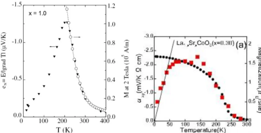
3.3.5 Ferromagnetic materials

In ferromagnets, the Hall resistivity ρ _xy decomposes into the sum of the normal Hall resis-

tivity, ρ ⁿ _xy = R ₀ B and the anomalous part, ρ ^a _xy = R _a M that is proportional to the magne-

tization [5860]. The anomalous Hall eect is furthermore distinguished between intrinsic

mechanisms, such as the Berry phase that leads to dissipationless currents [6163] and ex-

trinsic contributions like skew scattering ( ρ _xy ∝ ρ _xx ) [64] and side jump ( ρ _xy ∝ ρ ² _xx ). The

Figure 3.7: Left panel: Temperature dependence of the Nernst signal at 2 T for CuCr 2 Se 4−x Br x . Above T C e N scales with the paramagnetic magnetization M (2 T) [60]. Right panel: Temperature dependence of α _xy in La 0.7 Sr 0.3 CoO 3 , scaling with the ferromagnetic magnetization until saturation and decreasing nearly linear in temperature for lower T [58].

latter describes small displacement of a charge carrier being scattered by an impurity [65].

Analogous to the Hall eect the Nernst signal can also be decomposed into terms that are separately proportional to the magnetic eld and to the magnetization, e N = Q 0 B + Q a M [60]. In CuCr 2 Se ^4−x Br x as shown in Fig. 3.7 (left panel) the Nernst signal is found to scale with M (T ) above the ferromagnetic transition, interpreted as a signicant transverse electrical current caused by uctuations in the paramagnetic magnetization. In the work of Miyasato et al. [58] the o-diagonal Peltier coecient, α _xy is found to obey the Mott rule (Eq. (3.23)): α _xy increases just below the Curie temperature T _c proportionally to the mag- netization and after the magnetization saturates it decreases linearly with T until it goes to zero which can be well understood using (Eq. (3.23)). Just below T _c the band structure changes due to the ferromagnetic transition, enhancing the factor ( ∂σ _xy ()/∂) _F . After the magnetization is saturated, the T -linear term in (Eq. (3.23)) becomes dominant in the change of α _xy as shown in Fig 3.3.5 (right panel).

α _xy = π ² 3

k ² _B T e

∂σ xy

∂

F

. (3.23)

3.4 Nernst eect in the vortex liquid phase

The mentioning of this eect is a bit forestalled because it will cover the largest part of this work from the next chapter on. However, this small section completes the listing of dierent mechanisms that cause large Nernst eects. The basic Nernst signal in the mixed phase of high-temperature superconductors is given by the product of the nite transport entropy in the vortex core, s _Φ , and the ux ow resistivity ρ :

e _N ≈ ρ s _Φ

Φ ₀ = e ^s _N . (3.24)

Φ ₀ denotes the elementary ux quantum. A more detailed discussion of the vortex physics in a temperature gradient will be the content of section 4.2.5. Completing the above equation with the normal-state (metallic) Nernst signal derived in Eq. (3.16) yields the sum of both (assuming isothermal test conditions),

e _N = e ^s _N + e ⁿ _N = ρ s _Φ

Φ ₀ + ρ ⁿ α ⁿ _xy − S tan Θ. (3.25)

The aim of one part of this work is the systematic investigation of the evolution of the

vortex Nernst signal crossing the superconducting transition temperature of the Ni-doped

high-T c compound NdBa ₂ {Cu _1-y Ni _y } ₃ O 7 − δ . Therefore the separation of the supercon-

ducting Nernst signal from the normal state Nernst signal is crucial. Fortunately the

normal-state signal in the investigated system turned out to be a quasiparticle signal that

depends linearly on the applied magnetic eld while the vortex Nernst signal is highly

non-linear and therefore is easy to separate. An introduction into the physics of high-

temperature superconductors, the appearance of vortices and the generation of voltages in

the superconducting state will be given in the next chapter.

4.1 Introduction

Superconductivity was discovered by Heike Kamerlingh Onnes in 1911 [66] when he found that the electrical resistivity of mercury suddenly vanished when the temperature fell below a certain critical value, T _c = 4.2 K. The next hallmark was the discovery of an eect observed by Mei ß ner and Ochsenfeld [67] in 1933: A superconductor that is exposed to a magnetic eld at a temperature T > T c and is then cooled down below its critical temperature is able to expel the applied magnetic eld. This perfect diamagnetism or Mei ß ner eect together with zero resistivity characterize superconductors.

In 1986, a new class of superconductors were discovered by J. Bednorz and K. Muller [1]. These substances are ceramic compounds with critical temperatures ( T _c ) reaching as high as 138 K (Hg 0.8 Tl 0.2 )Ba 2 Ca 2 Cu 3 O 8.33 up to now. This property truly entitles these compounds with the name high-T c 's. A common structural feature of these substances are the copper-oxide (CuO) planes. It is believed that most of the physical properties including superconductivity are determined by mobile charge carriers that move within these planes. Since the CuO planes are separated by various other planes, such as i.e. LaO or BaO, most of theses structures can be addressed to as quasi-two-dimensional. These additional planes play structural roles and provide screening and doping environments.

The copper-oxide plane is a square lattice with copper ions being placed at the corners and oxygen ions placed at the center of the bonds that connect the copper ions. Because of those planes, the high-T c 's are also called cuprate superconductors. The research in the eld of the high-T c 's is mostly driven by the desire to unravel the origin of this special kind of superconductivity.

In this chapter, a brief introduction into the dierent types of superconductors, their phenomenology and some theories on superconductivity will be given with focus on the physics that is needed for the understanding of the thermomagnetic eects in high-T c 's [17, 6873].

4.1.1 Theoretical background

London theory

The London theory quantitatively describes the behavior of shielding currents and the

penetration depth of magnetic elds in surface sheets of superconductors. Since the exclu-

sion of the magnetic eld cannot happen discontinuously (implicating an innite current

density), the eld strength has to fall o within a certain typical length scale, λ ² _L = m _s

µ ₀ n _s e ² _s , (4.1)

that is called the London penetration depth. m _s , n _s and e _s relate to the mass, the density and the charge of Cooper-pairs [2], respectively. λ _L is derived from the London equations,

dj _s

dt = n _s e ² _s m s

E and ∇ × j _s + n _s e ² _s m s

B = 0. (4.2)

Ginzburg-Landau theory

The Ginzburg-Landau (GL) theory is based on Landau's theory of second-order phase transitions. The superconducting order parameter is dened as the wave function of the Cooper-pairs, Ψ(r) = |Ψ(r)|e ^iφ . The square of its absolute value is connected to the Cooper-pair density, |Ψ(r)| ² ∝ n _s . This density cannot discontinuously jump to zero at the surface of superconductors or at junctions between superconducting (s) and normal (n) conducting materials. To be descriptive, the length scale in which n s is allowed to vary spatially has to be at least the diameter of one Cooper-pair. This characterizing length scale is given by the coherence length, ξ . The characteristic length scales λ _L and ξ are visualized in Fig. 4.1. Within mean-eld theory, they obey the same temperature dependence in the vicinity of T _c , ξ(T ), λ _L (T ) ∝ (1 − t) ^−1/2 with t = T /T _c , so that it is reasonable to dene the Ginzburg-Landau-parameter,

κ = λ _L (T )

ξ(T ) . (4.3)

Typical values for a pure superconductor are in the range of λ _L ≈ 500 A and ξ ≈ 3000 A.

Assuming n s is reduced to zero within a length of ξ ≈ 3000 A, the loss of condensation energy of the superconducting phase is of the order of B _cth ² · ξ per unit of the s-n interface area ¹ . This loss on the other hand is a positive contribution to the surface energy. This surface energy is reduced again by B _cth ² · λ L , because the magnetic eld penetrates approx- imately 500 A into the superconductor. So, because of ξ > λ _L it would require additional energy to build up phase boundaries between superconducting and normal conducting zones, see Fig. 4.1.

The exact condition dening this so-called type-I superconductors is given by κ > 1

√ 2 type-I , (4.4)

characterizing materials that tend to expel magnetic elds completely. In case of ξ < λ _L , the superconductor tries to maximize the areas between superconducting and normal state

1 B _cth is the thermodynamic critical eld where the free enthalpy of the normal and the superconducting

states are of the same value.

Figure 4.1: Junction of normal (n) and superconducting material (s). The magnetic eld falls o on a typical length scale λ when entering the superconductor. The Cooper- pair density characteristically decreases on a length scale ξ when approaching the normal conducting region.

phases if a large enough magnetic eld is applied. In this case, magnetic ux in units of elementary ux quanta Φ ₀ = h/2e penetrates the bulk of the superconductor,

κ < 1

√ 2 type-II . (4.5)

Such a ux line is encircled by a superconducting ring current of Cooper-pairs and often re- ferred to as vortex. This phase is called mixed state or Shubnikov phase. The condition ξ < λ is easy to fulll by doping metallic impurities into a type-I superconductor. Doing so eects a decrease of the mean free path l which in turn makes the penetration length λ _L larger. Additionally, ξ ∝ √

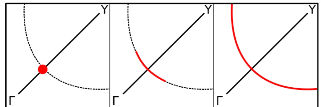
l . Two distinct magnetic eld regions now characterize the superconducting material. From B = 0 to B = B _c1 type-II superconductors expel the mag- netic eld just like a perfect diamagnet would do. B _c1 is given by B _c1 ≈ Φ ₀ /(πλ _L ) ² . From B _c1 to B _c2 ≈ Φ ₀ /(πξ) ² , magnetic ux tubes penetrate the bulk of the superconductor in units of Φ ₀ . At B _c2 the superconductivity breaks down which can be visualized as follows:

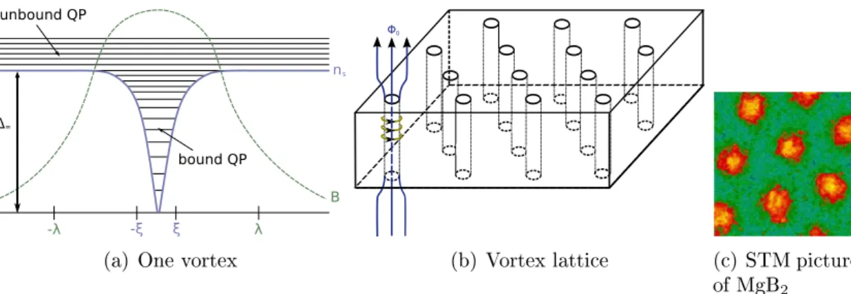
A ux tube covers the normal conducting area of ≈ πξ ² . The externally applied magnetic eld reects itself in the sum of single ux tubes that penetrate the sample, B = nΦ ₀ . If the ux tube density becomes so large, that the sum of their normal conducting cross sec- tion covers the whole sample, no superconducting areas are left. This behavior is depicted in Fig. 4.2. Furthermore, the ux lines in the mixed state are repelling each other. It was theoretically predicted by Abrikosov and later veried experimentally that they tend to arrange themselves in a regular triangular lattice, called Abrikosov lattice [74]. Such an arrangement is shown in Fig. 4.3 (b) and (c) while subgure (a) depicts the excitation spec- trum of one vortex together with its magnetic eld prole (governed by λ ) and its spatial variation of the superconducting density (governed by ξ ). The energy gap is denoted by

∆ ∞ .

Figure 4.2: Negative magnetization of type-I (dashed line) and type-II superconductors (solid line). B _c1 and B _c2 denote the lower and the upper critical elds, respectively.

B cth is the thermodynamic critical eld where the free enthalpy of the normal and the superconducting states are of the same value.

(a) One vortex (b) Vortex lattice (c) STM picture

of MgB 2

Figure 4.3: Illustration of magnetic ux penetrating the bulk of a type-II super-

conductor. (a) Scheme of one vortex of diameter 2 ξ : the normal conducting core

carries bound quasiparticles (QT) while outside the core live excitations from the

superconducting ground state that are unbound quasiparticles (at nite tempera-

ture). n _s and the magnetic eld prole are schematically shown by the continuous

and dashed lines, respectively. (b) depicts the arrangement of a vortex lattice in a

typical type-II material. (c) shows the vortex lattice in MgB 2 as observed by STM

[75].

BCS theory

A microscopic theory of superconductivity has been proposed by Bardeen, Cooper and Schrieer (BCS)[76], stating that even a week attractive interaction between electrons causes the formation of bound pairs with equal momentum and opposite spin. Such an interaction could be mediated via lattice displacements of the positive charged lattice ions as represented in a simplied picture: A rst electron moving through the lattice distorts the surrounding ions while the second feels this altered electrical potential and is thereby eectively attracted to the rst electron. Such a Cooper-pair has a binding energy of

∆(T = 0) = 2 ~ ω _D e

−2

D( F )U , (4.6)

with U expressing the coupling between electrons and phonons and D( _F ) the density of states at the Fermi energy. At T = 0 K, all electrons are bound to Cooper-pairs of the same quantum state. The rst excited state above this condensate is occupied by quasiparticles of the energy E _gap = 2∆ . Increasing the temperature leads to a gradual excitation of quasiparticles until at T _c with ∆(T _c ) = 0 or n _s (T _c ) = 0 superconductivity breaks down. BCS theory predicts in case of weak electron-phonon coupling an energy gap of size E _gap (0) = 2∆(0) = 3.52k _B T _c and a temperature dependence (in the vicinity of T _c ) of

∆(T )

∆(0) = r

1 − T

T _c . (4.7)

4.1.2 Pinned and depinned vortices

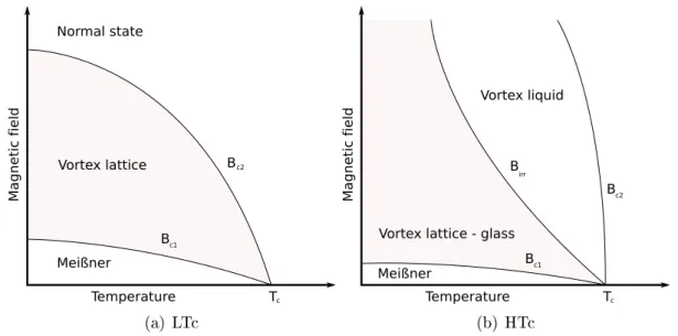
Starting from the development of equilibrium theory for the behavior of type-II supercon- ductors by Abrikosov [74] in magnetic elds, two categories of type-II superconductors can be distinguished. The rst category comprises the type-II superconductors described so far, e.g. impurity doped type-I superconductors with T _c < 26 K. Their typical B (T ) phase diagram is shown in Fig. 4.4(a). The vortex lattice above B _c1 spontaneously breaks two symmetries, namely phase coherence in the pairing eld and translational symmetry due to the development of long range order of the vortex lattice. One ux tube has an energy per unit length of = B _c1 Φ ₀ /µ ₀ . A ux tube can lower its energy by going through a normal state region within the bulk of the superconductor e.g. caused by metallic impurities just because the superconducting length of the ux tube is reduced. Thus, these areas tend to trap the ux line, a phenomenon called pinning. Consequently, such areas of static disorder will contribute to a nite pinning force density, f _p which is the pinning force per unit length of the ux line. f _p counteracts driving forces caused by application of currents or temperature gradients. Thermal uctuations cause disorder that aect the phase dia- gram as well as the dynamic properties [77, 78]. These uctuations tend to smooth the pinning potential which leads to thermal depinning of the ux line and thereby resulting in so called ux creep (thermally activated ux jumps from one pinning center to another).

Quantitatively, the strength of thermal uctuations may be expressed by the Ginzburg

(a) LTc (b) HTc

Figure 4.4: Schematic phase diagram of a type II LTc (a) and that of a type II HTc (b). B c1 and B c2 are the lower and the upper critical elds, respectively. B irr

in (b) is the irreversibility line, or melting line of the vortex lattice. Adapted from [71].

number, G = [2µ ₀ k _B T _c /(B _cth ² ξ _k ² ξ ⊥ )] ² /2 measuring the relative size of the transition tem- perature and condensation energy within a coherence volume. The phenomenological phase diagram showing the modications for a high-T c is presented in Fig. 4.4(b). Here T c and the Landau penetration depth are large, while the coherence length is very small. There- fore, these materials are governed by weaker pinning and signicant thermal uctuations, G ≈ 10 ⁻² compared to G ≈ 10 ⁻⁸ in low-T c superconductors. The experimental relevance is, that for type-II superconductors with low T _c 's, vortices are mostly pinned in the whole temperature and magnetic eld range accessible. In high-T c 's however, there is a distinct line separating reversible magnetic behavior and irreversible magnetic behavior. This is the irreversibility line B _irr (T ) . Above this line, vortices are free to move, resulting in reversible magnetization curves. The irreversibility line is also called depinning or melting line and is shown exemplarily for two samples of NdBa 2 {Cu 1-y Ni y } 3 O 7 − δ (0,3% Ni) in Fig. 4.5. It represents the eld strength and thereby the ux density which is necessary to overcome pinning forces at xed temperatures, in this case derived from Nernst eect measurements.

The vortex lattice melting from a low temperature ordered phase into a high temper-

ature vortex liquid is believed to be a thermodynamic phase transition [79]. Taking into

account the pinning disorder, a transition from the vortex-liquid into a vortex glass phase

is also possible, as proposed by Fischer et al. [80]. The consequence is that vortices at low

temperatures are frozen into random congurations.

20 30 40 50 80 90 100 0

2 4 6 8 10 12

MagneticField(T)

Temperature (K)

0% Ni, T c

~ 95K 3% Ni, T

c ~ 59K

Vortex

liquid

Figure 4.5: Vortex melting lines for two optimally doped samples of

NdBa 2 {Cu 1-y Ni y } 3 O 7 − δ with Ni contents of 0% and 3%. Data is extracted from

measurements of the Nernst signal. For given temperatures (only below the su-

perconducting transition temperature), a certain eld strength has to be passed to

generate voltages at the transverse contacts. This is then referred to as pinning

eld or melting eld B _m (T ) . The so extracted melting lines separate the vortex

lattice from the vortex liquid phase.

Figure 4.6: Voltage generation by vortex movement - scheme.

One circle around a ux line collects a phase of 2 π which is sym- bolized here by following the path along (i,-,-i,+). Moving vortices passing the reference points 1 and 2 produce a transverse electric eld because of time dependent phase slip processes, resulting in E = v × B .

4.2 Vortex dynamics

4.2.1 Voltages in high-T ^c materials

As mentioned before, superconductors are mainly characterized by two basic features:

perfect diamagnetism and a vanishing resistivity. The latter makes sure that no voltages can be developed because they will be immediately bypassed by a superconducting current.

Nevertheless, resistive behavior can be observed in the mixed phase, once the melting line has been overcome. All following discussion will be based on the assumption that the magnetic eld is directed perpendicular to the CuO planes. Because only within these planes supercurrents are able to encircle the magnetic eld. A conguration with the magnetic eld directed parallel to the planes would result in a scenario where charge carriers tunnel from plane to plane in c direction, thereby creating a vortex-like structure referred to as Josephson-vortex. The vortices oriented perpendicular to the planes can easily be forced to move through the sample by either applying a transport current or a temperature gradient perpendicular to the applied magnetic eld. A moving vortex then produces a voltage perpendicular to its moving direction. Since a single ux line is surrounded by a supercurrent of Cooper-pairs, the continuity of their wave functions requires that the phase returns to itself modulo 2 π . Because of this phase singularity at each vortex core, the motion of vortices produces a phase-slippage voltage [81], U , which can be understood by the Josephson equation:

∂ ∆φ

∂t = 2eU

~ with ∆φ = φ ₁ − φ ₂ . (4.8)

∆φ denotes the phase dierence between two points 1 and 2 (Fig. 4.6).

As the ux lines cross a virtual line between 1 and 2, the average phase dierences can

be expressed by

∂∆Φ

∂t = 2πbvn, (4.9)

with b the distance between the two points, v the vortex velocity and n the vortex density, controlled by the applied magnetic eld:

n = B

Φ ₀ with Φ ₀ = h

2e . (4.10)

The consequence is an electric eld perpendicular to the vortex motion and the magnetic eld:

| E _y |= v _x B _z or E = v × B. (4.11)

4.2.2 Some forces on vortices

In this section the basic ideas of moving vortices will be introduced. The causes for vortex motion will be limited to two cases, namely vortex motion induced by a transport current and by an applied temperature gradient. Other mechanisms to make vortices move with respect to the lattice would e.g. be a timely modulation of the applied magnetic eld and others [68, 70, 73, 82]. Forces will be given in notation of forces per unit length, f = F/l . The vector z denotes the unit vector in z direction which is the direction of the magnetic ux in the vortex core. The discussion is based on a two uid scenario in which two kinds of charged particles are assumed to be spread within the bulk of the sample: the superconducting Cooper-pairs with density n _s and velocity v _s and the normal conducting quasiparticles with density n _n and velocity v _n .

Magnus force

Here the concept of the Magnus force that arises due to a moving vortex with respect to the surrounding superconducting liquid is discussed. The force can be derived as it is long known in classical hydrodynamics and nds its most prominent example in the lift force that the ow of air produces on a wing of a plane [83, 84]. The implications of this transverse force on moving vortices in a Bose superuid will be expatiated below. The Magnus force on a moving vortex rst appeared in the work of Nozieres and Vinen [85]

and is normal to the relative vortex velocity. It is therefore a reactive force and produces no work [84]. Assuming a vortex with uniform velocity v Φ and a current of the superuid far away from the vortex core, v _s . Together with the ux vector z which is directed parallel to the magnetic eld, the magnus force can be written as

f M = n _s h

2 (v Φ − v s ) × z, (4.12)

where n _s denotes the density of the superconducting uid.

The nomenclature for the Magnus force often diers in literature, i.e. Eq. (4.12) can also

be written as f _M = ⁿ ₂ ^{s h} v _Φ × z − ^{n s} ₂ ^h v _s × z . The rst term on the right side resembles the