A neuro-mechanical model for the switching of stepping direction and transitions between walking gaits in the stick insect

switching of stepping direction and transitions between walking

gaits in the stick insect

Inaugural-Dissertation

zur

Erlangung des Doktorgrades

der Mathematisch-Naturwissenschaftlichen Fakult¨at der Universit¨at zu K¨oln

vorgelegt von

Sascha Alexander Knops

aus Stolberg (Rhld.)

K¨oln, 2013

...

...

...

...

...

...

...

...

...

...

...

...

...

...

...

...

...

...

...

Berichterstatter:

Dr. Silvia Gruhn

Prof. Dr. Ansgar B¨ uschges

Tag der m¨ undlichen Pr¨ ufung: 9. April 2013

Der Herr aber liess einen Ostwind ins Land wehen jenen ganzen Tag und die ganze Nacht;

und als es Morgen ward,

hatte der Ostwind die Heuschrecken gebracht.

” Der Herr aber liess einen Ostwind ins Land wehen jenen ganzen Tag und die ganze Nacht;

und als es Morgen ward,

hatte der Ostwind die Heuschrecken gebracht.“

Exodus 10,13

In dieser Arbeit wird ein mathematisches Modell zur Fortbewegung der Stab- heuschrecke entwickelt, das physiologische Gegebenheiten ber¨ucksichtigt und eine Reihe von biologisch relevanten Eigenschaften nachahmen kann.

Das Modell basiert auf der Erkenntnis, dass sensorische R¨uckkopplung einen starken Einfluss auf die Koordination der Gliedmaßen hat. Zentrale Mus- tergeneratoren (CPGs) steuern den Rhythmus der Bewegung und werden durch sensorische Einfl¨usse zwischen den Segmenten geregelt. Die Aktivit¨at der CPGs wird ¨uber Motoneuronen auf die Muskeln ¨ubertragen.

Ausgehend von bereits bestehenden Neuronmodellen und neuronalen Netz- werkmodellen wird ein neuro-mechanisches Modell entwickelt, welches sowohl die Kopplung von Gliedmaßen innerhalb eines Beines als auch die Kopplung von verschiedenen Beinen umfasst.

Zun¨achst werden die mechanischen Modelle f¨ur die Bewegung der drei Ge- lenke, die im wesentlichen zu Fortbewegung beitragen, hergeleitet. Im An- schluss werden diese mechanischen Modelle mit einem neuronalen vereinigt und stellen somit ein neuro-mechanisches System f¨ur ein Einzelgelenk dar.

Durch sensorische Kopplung dreier Gelenke und mit Hilfe der Einf¨uhrung ei- nes Schaltmechanismus werden Vorw¨arts-, Seitw¨arts- und R¨uckw¨artsschritte eines Mittelbeines ausgef¨uhrt. Mit der Verkn¨upfung von zwei laufenden Mit- telbeinen an einen K¨orper mit starren Vorder- und Hinterbeinen werden Kur-

iv

venlaufsequenzen erzeugt. Nach der Erweiterung des Modells auf die Vorder- und Hinterbeine werden unter der Erzeugung verschiedener Gangarten ge- eignete intersegmentale sensorische Verbindungen getestet.

Es zeigt sich, dass die ¨ Anderung der Laufrichtung durch die ¨ Anderung eines

einzelnen zentralen Kommandos eingeleitet werden kann und dass w¨ahrend

des Kurvenlaufens eine st¨arkere Kr¨ummung durch ein r¨uckw¨artslaufendes

Mittelbein erzeugt werden kann. Es stellt sich heraus, dass die Gangarten

Tetrapod und Tripod sich durch schwache inhibitorische Verbindungen er-

zeugen lassen.

In this study, a mathematical model for the locomotion of the stick insect is developed. This model takes physiological conditions into account and it is capable of mimicking biological relevant features.

The model is predicated on the crucial role, that sensory feedback plays in the coordination of limbs during walking. Central Pattern Generators (CPGs), which produce the rhythm of locomotion, are affected by sensory influences between the segments. The activities of the CPGs are transferred by the motoneurons to the muscles.

Starting with existing neuron models and neuronal network models, a neuro- mechanical model is developed that includes the coupling of segments inside of a leg as well as the coupling of multiple legs.

Firstly, mechanical models concerning the motion of the three isolated main joints are derived. These mechanical models are fused with the neuronal one.

Thus, they represent neuro-mechanical models for the single joints that are coupled via sensory feedback. By means of the introduction of a switching mechanism the model is able to produce forward, backward and sideward stepping of a middle leg. Through the junction of two stepping middle legs to the body of the modeled stick insect, curve walking sequences with differ- ent curvatures can be produced. By extending the model to the front and the hind leg, the structure of intersegmental connection between the legs during

vi

the tripod and tetrapod gait can be generated.

The change of stepping direction can be brought about by changing one sin-

gle central command. If the middle leg is stepping backwards, the curvature

during turning is smaller than in the case of sideward stepping. Weakly

inhibitory intersegmental connections show the most accommodating leg co-

ordination during both the tetrapod and the tripod gait.

1 Introduction 1

2 Methods 6

2.1 Interneuron model . . . . 7

2.2 Motoneuron model . . . . 9

2.3 Muscle model . . . 11

2.3.1 Coordinate system in the stick insect . . . 13

2.3.2 Equation of motion for angle in the FTi-joint . . . 18

2.3.3 Equation of motion for angle in the CTr-joint . . . 23

2.3.4 Equation of motion for angle in the ThC-joint . . . 24

2.3.5 Determination of the spring constants . . . 26

2.4 Coupling leg segments . . . 28

2.5 Synthesis of neuronal and mechanical models . . . 40

2.5.1 A single joint . . . 40

2.5.2 Neuro-muscular coupling . . . 42

2.5.3 A single leg . . . 42

2.5.4 Multiple legs . . . 47

2.6 Implementation of the model . . . 52

3 Results 55

viii

3.1 The single joint system . . . 56

3.1.1 The mechanical motion . . . 56

3.1.2 The neuro-mechanical system . . . 59

3.2 Interjoint coupling in a single leg . . . 62

3.2.1 Middle leg . . . 67

3.2.2 Switching mechanism . . . 69

3.2.3 Neuronal basis of curve walking . . . 74

3.2.4 Applying the model to ipsilateral legs . . . 79

3.3 Intersegmental coupling - Multiple legs . . . 84

4 Discussion 96 4.1 Summary of the model structure and its properties . . . 96

4.2 Discussion of the results . . . 99

4.3 Comparison to existing models . . . 103

4.4 Biological significance of the model and outlook . . . 106

A Summary of the model parameters 109 A.1 Neuron models . . . 109

A.2 Mechanical models . . . 117

B Simulation with the coupled femur and tibia 125

Introduction

Locomotion of arthropods and various vertebrates is based on the coordi- nated movement of leg joints. This movement can be subdivided into two phases: one in which the leg has ground contact and another in which it is lifted off the ground. The former is called stance phase and the latter is named swing phase. During forward walking the stance phase begins with the touch-down of the tarsus at its anterior extreme position (AEP). Accord- ingly, the body is propulsed while the leg moves relatively to the thorax to the posterior extreme position (PEP). Subsequently, the lift-off of the tar- sus commences the swing phase. The leg is moved to its AEP and a new stepping cycle begins. The neuronal and mechanical control of several com- ponents is crucial for the coordination of leg joints and different legs between each other. The muscular and neuronal mechanisms, involved in arthropod locomotion, have been thoroughly studied in the stick insect (Carausius mo- rosus ) (B¨assler and B¨ uschges, 1998; B¨ uschges et al., 2008, 2011; D¨ urr et al., 2004; Orlovsky et al., 1999; Ritzmann and B¨ uschges, 2007). In many insects walking patterns are generated decentralized. Central neuronal net- works generate basic motor activity that is influenced by sensory feedback.

1

That means, sensory feedback plays an essential role in the shaping of motor output and in the control of stance and swing phase. The sensory signals are: movement and position signals from the leg joints on the one hand and force and load signals from the leg segments on the other hand (Borgmann et al. 2011; Daun-Gruhn et al. 2011; Zill et al. 2004; Zill et al. 2009; Zill et al.

2011; for a review see B¨ uschges and Gruhn 2008). Leg joints are driven by their individual pattern generating networks (CPGs). These CPGs activate pools of motoneurons that innervate muscles in the respective joints (Akay et al., 2004; B¨ uschges, 1995, 1998, 2005).

The intersegmental coordination of legs has been investigated on the behav- ioral level (Cruse, 1990; Graham, 1972; von Buddenbrock, 1921; Wendler, 1965, 1978) as well as on the neuro-muscular level by recording EMG activ- ity, intracellular and extracellular electrical activity of motoneurons (MNs) (B¨ uschges, 1995; B¨ uschges et al., 2004; Ritzmann and B¨ uschges, 2007; B¨ uschges et al., 2008; Borgmann et al., 2009; Rosenbaum et al., 2010).

Leg coordination during stepping is subdivided into different walking gaits.

While insects walk at high velocities, they adopt a symmetric tripod gait.

Three legs are lifted off and three legs have ground contact at the same time

(Delcomyn, 1971). At low velocities or under load conditions they adopt an

asymmetric tetrapod gait. Two legs are lifted off while four legs have ground

contact (Graham, 1972). The coordination of legs in gait generation has

been studied carefully in behavioral experiments (Cruse, 1990; Delcomyn,

1989; D¨ urr et al., 2004; Grabowska et al., 2012). Furthermore, the investiga-

tion of video records with regards to free walking stick insects revealed that

irregular gaits were mostly due to multiple stepping in the front legs. These

findings lead to the assumption that the front legs carry out a searching

function and that they are not coupled to the middle legs. However, middle

and hind leg coordination by themselves show regular gaits comparable to quadrupedal walk and wave gaits. These characteristics are retained in front leg amputees.

Details of neuronal and mechanical properties of a forward stepping single leg are well-investigated (B¨ uschges, 2005; B¨ uschges et al., 2008; D¨ urr et al., 2004; Orlovsky et al., 1999). These findings made it possible to build con- trollers of the single joint and single leg of the stick insect (Ekeberg et al., 2004) as well as the cat hind leg (Ekeberg and Pearson, 2005; Pearson et al., 2006). Such details for backward and sideward stepping and the neuronal basis for gait generation have remained largely unknown.

One way to gain insight into underlying mechanisms is to create appropriate mathematical models. There are different types of models existing that focus on different aspects of locomotion in animals. There are models concentrat- ing on bio-mechanical properties in locomotion (Holmes et al., 2006), models that center on the role of chains of centrally coupled oscillators in locomotion (Ijspeert et al., 2007), models focusing on behavioral studies (Cruse, 1990) and models that give attention to the role of sensory signals in the coordina- tion of legs during locomotion based on neuro-physiological studies (Ekeberg and Pearson, 2005; Ekeberg et al., 2004).

The first two kinds of models investigate the generation of rhythmic activity by neuronal properties and the synchronization of the network by interneu- rons. These investigations are aiming at the explanation of the affection of synchronization at different oscillator couplings and different intrinsic fre- quencies rather than the explanation of rhythmogenesis. The third kind of model concerns discontinuous bistable systems and spares the use of CPGs.

Such reflex chains have two stable steady states for the same set of parame-

ters. The switch between these two states is controlled by an input param-

eter. The fourth kind of model takes neuro-physiological experiments into account. Certainly, it does not make use of CPGs. Therefore, the generation of periodic motor output is not possible in the latter two models.

An alternative approach is taken by a model by Daun-Gruhn (2011): Accord- ing to that CPGs are connected by biologically-inspired synapses modulated by sensory input. This model is extended by taking experimental findings on intersegmental influences (Borgmann et al., 2007, 2009; Ludwar et al., 2005) into account. It aims at elucidating basic neuronal processes during transitions of gaits. These processes are an outcome of sensory influences.

Changes are only required in the central drives to the CPGs (Daun-Gruhn and Toth, 2011). In Toth et al. (2012) a model for a single middle leg with two joints is constructed. It includes a neuro-mechanical model that explains the conversion of rhythmic electrical CPG activity into mechanical leg move- ment. Originally, this neuro-mechanical model only includes the coupled system of the Thorax-Coxa-joint (ThC-joint) and the Coxa-Trochanter-joint (CTr-joint). At the ThC-joint the protractor coxae and the retractor coxae muscle pair moves the coxa forward and backward. At the CTr-joint the lev- ator trochanteris and the depressor trochanteris muscle pair moves the femur up and down. Nevertheless, the Femur-Tibia-joint (FTi-joint) about which the tibia is flexed or extended by the flexor tibiae and the extensor tibiae muscle pair is not included. The model is capable of producing forward and backward stepping and switching between them by changing a single neu- ronal signal.

This study treats of the further development with regard to the neuro-

mechanical model by Toth et al. (2012), which is mentioned above. It also

comprises the embedding of an intersegmental coupled network of three ip-

silateral legs similar to the model in Daun-Gruhn and Toth (2011). The

novelties in this work are as follows: i) the coupling of the FTi-joint to the existing two joint model (Knops et al., 2012), ii) the capability of sideward stepping through the attachment of the FTi-joint (Knops et al., 2012), iii) the explanation of basic neuronal mechanisms of curve walking through the application of sideward stepping and backward stepping (Knops et al., 2012), iv) the construction of an ipsilateral three-leg model including properties of the neuro-mechanical model, v) the generation of gaits and vi) the transition between gaits.

In this study, chapter 2 presents the methods and techniques used in the construction, implementation and simulation of the aforementioned models.

The description of the basic properties of these models and the simulation re-

sults achieved with them are presented in chapter 3. In connection with this

the results are summed up and discussed in chapter 4. Appendix A presents

a concise summary of the model parameters and their numerical values used

in the models. Appendix B shows the simulation results obtained with the

mechanically coupled femur and tibia.

Methods

This chapter concerns the development of a neuro-mechanical model for the locomotion in the stick insect and it provides a recollection of necessary mathematical tools that are already established. In sections 2.1 and 2.2 the original interneuron and motoneuron models are summarized (cf. Daun- Gruhn (2011); Daun-Gruhn et al. (2011)). The derivation of the mechanical equations of motion for all three main leg joints is presented in section 2.3.

After fixing the coordinate system in section 2.3.1 the equation of motion in the FTi-joint is derived in section 2.3.2 (see also Knops et al. (2012)).

Pertaining to the other two joints (CTr-joint and ThC-joint), the derivation of the equation of mechanical motion is summarized on the basis of Toth et al.

(2012) in sections 2.3.3 and 2.3.4. Section 2.3.5 the dynamical parameters in all three main joints are determined by a procedure that was first published in Toth et al. (2012). How the equation of motion concerning a coupled system of the CTr-joint with the FTi-joint can be deduced is shown in section 2.4.

The synthesis of mechanical and neuronal models and a successive buildup of a three-legged locomotor system is performed in section 2.5. Section 2.5.1 refers to the single joint system (Toth et al., 2012) and section 2.5.3 relates

6

to the coupled three-joint system (Knops et al., 2012). The intersegmental neuronal connection between three ipsilateral legs on a neuro-mechanical basis is presented in section 2.5.4. This chapter concludes with technical comments about the implementation of the model in section 2.6.

2.1 Interneuron model

There are two features observed in CPGs: endogenously bursting neurons and

mutually inhibitory connections (Calabrese, 1995; Satterlie, 1985; Selverston

and Moulins, 1985). Rhythmic activity is produce on the level of basal excita-

tory activity and on the level of patterning by inhibitory coupling (Grillner

et al., 2005). For that purpose, Daun-Gruhn (2011) modeled a CPG as

two Hodgkin-Huxley-type neurons mutually coupled by inhibitory synapses

(Hodgkin and Huxley, 1952). Due to its mutual inhibition, neurons are or-

ganized into two antagonistic groups (Izhikevich, 2007). The neurons carry

a slowly-inactivating sodium current and they are tuned such that they are

tonically active without coupling. Actually, this current is present in most

neuron types and it is shown in Daun et al. (2009) that the sensitivity of the

oscillation period to variations of the excitatory input as well as the degree

to which the phase can be separately controlled, strongly depend on intrinsic

cellular mechanisms that are involved in rhythmogenesis and phase transi-

tions. The usage of a slowly-inactivating sodium current leads to the widest

range of oscillation periods and the greatest degree of independence of phase

duration control at asymmetric inputs (Daun et al., 2009). Despite of that

there is not much known about the compositions of the currents in the stick

insect (Westmark et al., 2009), slowly-inactivating persistent currents play

an important role in neuronal networks of other animals (Katz and Hooper,

2007; van Drongelen et al., 2006; Zhong et al., 2007).

The electrical activity of the non-spiking interneurons (CPG neurons and other interneurons) is described by the following equation system:

C

dV

dt = − (I

+ I

+ I

+ I

) I

= g

m

(V )h(V − E

)

I

= g

(V − E

)

I

= g

s

(V

)(V − E

) I

= g

(V − E

)

dh

dt = (h

(V ) − h)/τ

(V )

with V = V (t) being the membrane potential, g

being the maximal conduc- tances of the membrane currents, E

being the reversal potential, C

being the membrane potential. h = h(t) denotes the inactivation variable of the slowly-inactivating sodium current I

. The function m

(V ) is the steady- state value at V of the activation variable m of I

, the function h

(V ) is the steady-state value at V of the inactivation variable h of I

and the function s

(V

) is the actual value of the synaptic activation induced by another cell with membrane potential V

. The latter three functions enunciated in the following formula:

z

(V ) = 1

1 + exp γ

(V − V

) (2.1)

with z = m, h, s. The sensory input to the interneurons is represented by

the applied current I

and the strength can be tuned by varying g

. This

is relevant with reference to the adjustment of the oscillatory period and the

phase relation of CPG neurons. The parameters for all interneurons and

synapses used here are listed in tables A.2 - A.3 of Appendix A.

2.2 Motoneuron model

The motoneurons are modeled by a Hodgkin-Huxley type neuron model (Hodgkin and Huxley, 1952) as well. In contrast to the interneuron model, these neurons produce proper action potentials and exhibit adaptive behav- ior, i.e. decreasing firing frequency during sustained stimuli. These properties can be achieved by the use of four intrinsic ionic membrane currents: the fast inactivating sodium current I

, the delayed rectifier potassium current I

, an outward (potassium) current I

responsible for the adaptation of firing, and the leakage current I

(Daun-Gruhn et al., 2011). A synaptic current I

and an applied current I

introduced in section 2.1 are included, too.

The currents I

and I

are adapted from Traub et al. (1991). The mo- toneuron model used in this study is taken from Toth and Gruhn (2011), and the basic equations are

C

dV

dt = − (I

+ I

+ I

+ I

+ I

+ I

) (2.2) with

I

= g

m

h

(V − E

) (2.3)

I

= g

m

(V − E

) (2.4)

I

= g

m

(V − E

) (2.5)

I

= g

(V − E

) (2.6)

I

= g

s

(V

)(V − E

) (2.7)

I

= g

(V − E

) (2.8)

g

being the maximal conductances of the membrane currents, E

being the reversal potential and i = N a, K, q, syn, app. The inactivation variable h

and the activation variable m

, respectively, are described by dy

dt = α

(V )(1 − y) − β

(V )y (2.9)

where y = h

, m

, m

. The coefficients α(V ) and β(V ) are non-linear functions of the membrane potential V , depending on the membrane current.

For the activation variable m

in the sodium current I

, there is α

= a

(a

− V )

exp (a

(a

− V )) − 1 (2.10) β

= b

(b

− V )

exp (b

(b

− V )) − 1 (2.11) For the inactivation variable h

in the sodium current I

, there is

α

= a

exp (a

(a

− V )) (2.12) β

= b

exp (b

(b

− V )) + 1 (2.13) The numerical values of the parameters can be found in table A.5 in the Appendix A.

For the activation variable m

in the potassium current I

, there is α

= a

(a

− V )

exp (b

(b

− V )) − 1 (2.14) β

= b

exp (b

(b

− V )) (2.15) The numerical values of the parameters can be found in table A.6 in the Appendix A. Note, that the potassium current is not inactivating and thus the inactivation variable h does not appear in its equation.

The adaptation current I

leads to a decrease of firing frequency in the mo- toneuron at sufficiently long stimuli. For the activation variable m

one has

m

dt = r

(m

(V ) − m

) (2.16)

m

= 1

1 + exp (s

(V − V

)) (2.17)

r

= const (2.18)

where m

is the steady-state value of m

at V . The numerical values of the

parameters can be found in table A.7 in Appendix A.

The parameters concerning the leakage current I

are listed in table A.8 in Appendix A.

2.3 Muscle model

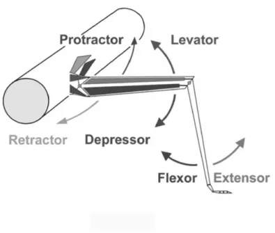
In this section, it is shown how the equations of motion, relating to mechan- ical movement, can be deduced. This is carried out explicitly for the FTi joint as it appears in Knops et al. (2012). It is a proceeding work concerning the extension of an existing neuro-mechanical model for the two proximal joints sited in the ThC and CTr (cf. Toth et al. (2012). The equations for the latter two joints are repeated briefly. A detailed description can be found in Toth et al. (2012). The femur-tibia joint (FTi-joint) is driven by flexor- extensor muscle pair (see figure 2.1). In the following, the expressions FE system and FTi-joint are treated as synonyms. The same applies to the LD system (CTr-joint) and the PR system (ThC-joint).

The mechanical motion of a single joint in the stick insect is brought about

by the activity of antagonistic muscles. In a single leg, there are three such

muscle pairs (each located at a respective joint) that in essence produce the

locomotion of the insect. At the Thorax-Coxa-joint (ThC-joint) the protrac-

tor coxae and the retractor coxae (henceforth protractor-retractor) muscle

pair moves the coxa forward and backward, at the Coxa-Trochanter-joint

(CTr-joint) the levator trochanteris and the depressor trochanteris (hence-

forth levator-depressor) muscle pair moves the femur up and down, and at

the Femur-Tibia-joint (FTi-joint) the tibia is flexed or extended by the flexor

tibiae and the extensor tibiae (henceforth flexor-extensor) muscle pair. The

model for all the muscle pairs constructed here are based on the same prin-

ciples, which are a simplification of the Hill model (Hill, 1953). The simpli-

Figure 2.1: Schematic illustration of the leg joints and the basic movement directions.

Adapted with permission from M. Gruhn.

fication is done by the consolidation of all active and passive elastic muscle properties (cf. figure 2.2 A) into a single spring with variable elasticity mod- ule, i.e. spring constant (cf. figure 2.2 B). Guschlbauer (2009) found out that the muscles obey a non-linear elasticity law

F = k(l − l

)

(2.19)

for the muscle force F with the variable spring constant k, actual length l

and minimal length l

of the muscle.

k _s k _p

b _v

ACU

A k _ae

b _v

B

Figure 2.2: A: Hill’s muscle model and B: simplified muscle model used. In A, k

: modulus of the passive parallel elasticity, k

: modulus of the passive serial elasticity, b

: viscosity coefficient characterizing the viscosity of the muscle, ACU: active contraction unit respon- sible for the development of (isotonic or isometric) contraction force. The model illustrated in map B is obtained by omitting the passive serial elasticity, and by merging ACU with the passive parallel elasticity. Thus in B, k

: variable modulus of the active, nonlinear elasticity, b

as in A. Picture taken from Toth et al. (2012) with permission.

2.3.1 Coordinate system in the stick insect

The motion of a joint is characterized by the change of the respective joint

angle. These angles are (from proximal to distal): α in the ThC-joint, β

in the CTr-joint and γ in the FTi-joint. A front and plan view of the stick

insect’s leg is shown in figure 2.3. The coxa-trochanter and the femur are

merged to a simplified femur, since it has a negligible length and mass.

A

B

A i

A ii

C

D

posterior dorsal

levator extensor

depressor flexor

ventral

anterior retractor

protractor

FRONT VIEW

PLAN VIEW

tibia femur

Figure 2.3: Front view (A) and plan view (B) of the stick insect’s middle leg. The femur

and the tibia are moved by the protractor-retractor coxae, levator-depressor trochanteris,

and extensor-flexor tibiae B¨ assler (1983).

The angular movement of the angle α is generated by the protractor- retractor muscle pair. The range of the angular motion is determined by the anterior extreme position (AEP) and posterior extreme position (PEP).

The zero position of α is when the femur is bent forward and parallel with

the thorax (see figure 2.4). Consequently, the rearmost position eventuates

when the femur is parallel with the thorax corresponds to the angle α =

180

. These extreme positions are unlikely to occur in natural conditions

during locomotion of the stick insect. Hence they do not appear in the

simulations. The levator-depressor muscle pair moves the femur up and down

(angle β) between the extremal angles determined by the ground contact

during the stance phase and the highest elevated position of the femur during

the swing phase. The angle β = 0

is attained if the femur (or more precisely

trochanter-femur) will align with the coxa segment. One should keep in mind

that the coxa is declined downwards from the y-axis by an angle ψ (figure 2.5

A). The motion of the angle γ is mainly determined by the flexor-extensor

muscle pair. Thereby the tibia can be moved towards or away from the

body. At the angle γ = 0

the leg is fully stretched. At γ = 180

the tibia

is parallel to the femur, a non-physiological position (figure 2.5 B).

α = 0

femur

rostral

caudal

thorax α

y

x

Figure 2.4: Top view on the thorax of the stick insect and the walking plane in the

coordinate system used for the simulation. The rostral part is situated in the positive

direction of the x-axis and the caudal part in the negative direction. The angle α increases

with a caudal movement of the femur.

z

y

ψ β

dorsal

ventral

femur

β = 0

thorax

thorax femur

tibia

γ = 0 γ

dorsal

ventral

A

B

Figure 2.5: Front view on the thorax of the stick insect in the coordinate system used for

the simulation. A: β increases with dorsal movement of the femur. The zero-point of β

is given by the declination of the y-axis by the angle ψ. B: γ measures the flexion of the

tibia relative to the femur. The zero-position is achieved for an outstretched tibia and the

angle increases with the flexion of the tibia.

2.3.2 Equation of motion for angle in the FTi-joint

In this section, the equation of the angular movement γ in the FTi-joint will be derived when the other two angles (α and β) are kept constant. The derivation follows the one in Knops et al. (2012). Figure 2.6 A shows the geometrical arrangement of the extensor-flexor (FE) muscle system. The tendon of the extensor T

is fixed to the tibia at point A. The tendon of the flexor T

at is fixed at point B. The rotation axis of the tibia is at O.

It is perpendicular to the plane of the figure. It is known (Guschlbauer et al., 2007; Guschlbauer, 2009) that AO = d and BO = 2d. The tendons are moved by contraction of the muscle fibers, one of their ends fixed to the tendon, the other one to the cuticle (oblique lines between C

and T

, and C

and T

, respectively). The zero position of the angle γ is when the femur and the tibia are collinear, i.e. at outstretched leg. In figure 2.6 B a single muscle fiber is schematically displayed. The distance between tendon and cuticle is EG = h. The fiber is fixed to the tendon at point C, and to the cuticle at point G. In this position, it has length l

, and its angle with the tendon is φ

. If the muscle contracts (with a force F

), point C of the muscle fiber at the tendon will be shifted to point D, due to the force F

parallel to the tendon. The angle between tendon and fiber at D is φ. The angle γ between femur and tibia is thus determined by the movement of the tendon. Experiments by Guschlbauer (cf. Knops et al. (2012)) show that variation of h at different angles γ in both the flexor and the extensor is negligible (cf. figure 2.7). The distance h between the tendon and the cuticle is therefore considered to be constant during contraction. The mean value of this distance is h

= 0.34 mm for the extensor, and h

= 0.42 mm for the flexor. The equation of mechanical motion of the tibia reads

I

γ ¨ = F

· 2d sin γ − F

· d sin γ + M

(2.20)

with the moment of inertia I

, the parallel forces F

and F

in the flexor and the extensor muscles, and the distances 2d and d from the rotation point of the FTi-joint. M

is the torque due to viscosity that is produced by two force components acting on the lever:

M

= 2dF

+ dF

= − 2db

v

− db

v

= − 4d

b

γ ˙ − d

b

γ ˙

= − 5d

b

γ ˙ (2.21)

since the viscosity force is proportional to, and counteracts the velocity. The viscosity constant b

is set to be the same for both muscles. The equation of motion for the angle in the FTi-joint finally reads

¨ γ = d

I

[(2F

− F

) sin γ − 5b

d γ] ˙ (2.22) The forces F

= F

(l

) and F

= F

(l

) are the projections of the corresponding muscle forces on the direction of movement of the tendon:

F

= F

cos φ

(2.23)

F

= F

cos φ

(2.24)

where φ

= φ

(l

) and φ

= φ

(l

) are angles between the fibers and tendons in the respective muscles and depend on the fiber length. According to findings by Guschlbauer et al. (2007); Guschlbauer (2009) (cf. equation (2.19)), the muscle forces are quadratic functions of the muscle length:

F

= k

(l

− l

)

(2.25)

F

= k

(l

− l

)

(2.26)

l

and l

are the minimal lengths of the fibers, i.e. the lengths when

the fibers are unstrained. Since the muscle fibers are arranged in parallel, the

spring constants k

and k

of the entire muscles are the sum of individual fiber spring constants. The fiber length is calculated by using the cosine theorem

l

(γ) = q

l

+ s

(γ) − 2l

s

(γ) cos φ

and (2.27) l

(γ) =

q

l

+ s

(γ) − 2l

s

(γ) cos φ

(2.28) with cos φ

= p

1 − (h

/l

)

and cos φ

= p

1 − (h

/l

)

and the shifts

s

(γ) = − 2d sin γ and s

(γ) = d sin γ. l

and l

are fiber lengths, φ

0 and

φ

0 are the corresponding angles at γ = γ

= 90

.

γ A

B O C _E

T _E T _F C _F

A

Tendon Cuticle

l ₀ h

F p

F m

C D

E G

l

φ φ ₀

B

tibia femur

Figure 2.6: A: Geometric arrangement of the flexor and extensor muscles. The extensor tendon T

is fixed to the tibia at point A, and the flexor tendon T

at point B. The extensor muscle fibers (thick oblique lines), arranged in parallel, mechanically connect T

with the cuticle of the extensor C

. Similarly, the flexor fibers do so between T

and the flexor cuticle C

. The tibia rotates, with angle γ, about the axis at point O. This axis is perpendicular to the plane of the figure. B: Geometrical arrangement of a single muscle fiber between tendon and cuticle, and muscle forces. The fiber is fixed to the cuticle at point G. l

: length of the muscle fiber when its other end is at position C (reference length); l: its length at point D (generic length); h: distance between tendon and cuticle;

φ

and φ: angles corresponding to the positions at C and D, respectively. F

: muscle force in the fiber at point D (length l); F

: parallel component of F

moving the tendon.

This figure appears as it is in Knops et al. (2012).

0.0 0.1 0.2 0.3 0.4 0.5

med. 150°

med. 90°

prox. 90° prox. 150° med. 0°

Extensor tibiae

prox. 0°

N=6

h = Distance between tendon and cuticle [mm]

A

0.0 0.1 0.2 0.3 0.4 0.5

N=6

h = Distance between tendon and cuticle [mm]

Flexor tibiae

prox. 0° prox. 90° prox. 150° med. 0° med. 90° med. 150°

B *

Figure 2.7: Boxplots of the distance h between tendon and cuticle edge versus the angle at the FTi-joint for the medial and the proximal regions of the muscles for three different flexion angles (0

, 90

and 150

). A: extensor tibiae muscle, B: flexor tibiae muscle. In each box: data are obtained from the same 6 animals, Upper edge: 75 percentile; bottom edge:

25 percentile; line: median; small black square: mean value. Data from C. Guschlbauer,

published in Knops et al. (2012).

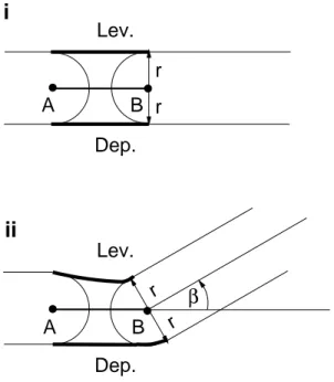
2.3.3 Equation of motion for angle in the CTr-joint

In this section, a brief description of the equations of mechanical motion at the CTr-joint is given (cf. Toth et al. (2012)). The angle α is kept constant and the tibia is omitted. Figures 2.8 (i) and (ii) show the geometrical arrangement of the levator-depressor (LD) system in the CTr-joint. The basic idea is that both muscles have the same length d, if the coxa-trochanter section is fully stretched. If the femur is moved up and down it will rotate about an axis at B , perpendicular to the plane of the figure. One of the muscles is elongated along the perimeter with the radius r and the center at B . The other muscle is shortened by the same amount. The actual lengths of the levator and depressor muscles are function of the rotation angle β and read

l

= d − rβ (2.29)

l

= d + rβ (2.30)

The equation of motion is

I

β ¨ = r(F

− F

− F

) (2.31) where I

is again the inertial momentum of the femur, ¨ β is the angular acceleration (second time derivative of the angle β) and F

and F

are the levator and depressor elastic muscle forces. Anew, according to equation (2.19) the muscle forces obey

F

= k

(l

− l

)

(2.32)

F

= k

(l

− l

)

(2.33)

with the viscosity force F

= b

v = b

r β ˙ and the viscosity coefficient

b

for the LD system. The final form of the equation of mechanical motion

Dep.

Lev.

r r

A B

i

Dep.

Lev.

r r

A B

β ii

Figure 2.8: Two geometric situations of the levator-depressor joint are shown. In i) the system is in fully stretched state (a non-physiological situation) when both muscles are assumed to have the same length: the distance between the points A and B, d = AB. The femur is on the right hand side. It hinges about the axis through the point B, orthogonal to the plane of the figure. In ii), the femur is tilted upward by an angle β. The shortening of the levator and the elongating of the depressor muscle (Toth et al., 2012).

in the LD system then reads

β ¨ = c

(F

− F

) − c

β ˙ (2.34) with c

= r/I

and c

= b

r

/I

.

2.3.4 Equation of motion for angle in the ThC-joint

In this section, a brief description of the equations of mechanical motion

in the ThC-joint is delivered (see Toth et al. (2012)). Figure 2.9 shows the

geometrical arrangement of the protractor-retractor system (PR) in the ThC-

joint. The rotation axis of the ThC-joint (thick black point) is perpendicular

r r

d F _R

l _R

l _P F _P φ _P φ _R

π−α α

Figure 2.9: Top view of the simplified geometrical arrangement. The posterior-anterior direction is the one from up to down — the same as in figure 2.3 B. The thick black line represents the thorax, while the unfilled rod the femur. The angle α characterizing the position of the femur is counted from anterior to posterior (as indicated). F

and F

are the forces in the retractor and protractor muscle, respectively. The corresponding muscle lengths are l

and l

(Toth et al., 2012).

to the plane of the figure and is the junction of the thorax (thick black line) and the femur (empty rod). The forces F

for the protractor and F

for the retractor are represented by the thick arrows. The muscles have the lengths l

and l

, respectively and attain the angles φ

and φ

, respectively between the muscle fibers and the femur. In this simplified model the muscles join the femur a the same distance d from the rotation point, and they join the thorax at the distance r. The equation of motion reads

I

α ¨ = F

d sin φ

− F

d sin φ

− F

d (2.35)

with the moment of inertia I

of the femur, the angular acceleration ¨ α, the muscle forces

F

= k

(l

− l

)

(2.36) F

= k

(l

− l

)

(2.37) obeying equation 2.19 and F

= b

v = b

αd ˙ the viscosity force that is assumed to be linearly proportional to the actual velocity v = ˙ αd. Herein

˙

α is the angular velocity and b

is the viscosity coefficient for the PR system. The sine theorem for triangles yields

I

α ¨ = rd sin α F

l

− F

l

− b

d

α ˙ (2.38) and the cosine theorem the actual muscle lengths l

and l

become functions of α:

l

= r

+ d

+ 2rd cos α (2.39) l

= r

+ d

− 2rd cos α (2.40) Finally, the equation of motion for the angle α reads

¨

α = c

sin α F

l

− F

l

− c

α ˙ (2.41)

with the constants c

= rd/I

and c

= b

d

/I

.

2.3.5 Determination of the spring constants

This section deals with the determination of spring constants first published

in Toth et al. (2012). The movement of the limbs is associated with the

change of respective joint angles driven by antagonistic muscles. In a periodic

and cyclic motion each joint angle moves in a certain range. The direction of

the angular motion is determined by the time courses of the muscle forces.

Therefore, a change in direction is due to a switch in the contraction forces.

This is gained by a change in spring constants (cf. equation (2.19)). The switch time is controlled by the CPG and it takes place at stationary points of the movement, i.e. where the angular velocity and the angular acceleration vanish (Toth et al., 2012). The dynamics of the muscles have to be set such that the joint angle reaches its extremal value by the time of the switch in the CPG. The dynamics are determined by the spring constants and viscosity.

For the angle in the FTi-joint at time T

, one has

γ(T

) = γ

, γ(T ˙

) = 0, and ¨ γ(T

) = 0 (2.42) These conditions used in equations (2.22), (2.25) and (2.26) lead to the fol- lowing ratio of the spring constants:

a

= k

k

= 1 2

(l

− l

)

cos φ

(l

− l

)

cos φ

(2.43) The lengths l

, l

and angles φ

, φ

are functions of the angle γ. As there are two extreme angles γ

(maximum flexion and maximum extension), it leads to two different values for a

: one for the flexion and another for the extension, where the angle at which the switch takes place has to be substituted into equation (2.43).

Analogously, the same procedure can be done for the angle β (by using equations (2.34), (2.32) and (2.33)):

a

= k

k

=

d − rβ

− l

d + rβ

− l

(2.44) with the extremal angle β

in the CTr-joint and for the angle α (by using equations (2.41), (2.36) and (2.37))

a

= k

k

= l

(α

) l

(α

)

(l

(α

) − l

)

(l

(α

) − l

)

(2.45)

with the extremal angle α

in the ThC-joint. The determination of the numerical values of the spring constants and the viscosity coefficient has to be accomplished by computer simulations (see section 3.1). In these simulations, only the equation of the mechanical (angular) motion is used. Consequently, the switch times are predetermined.

2.4 Coupling leg segments

So far, the equations of mechanical motions (angular movements) for the three isolated joints (muscle systems) are derived. However, due to mechan- ical coupling of the leg segments the motion of one joint can influence the motion of the others. For example, if the tibia moves, changing the angle in the FTi-joint, a force will be effective on the femur, too. This influence is most obvious for the CTr-joint since the local angles are in the same plane, i.e. their rotation axes are parallel. In general, the movement of the femur mechanically interacts with the movement of the tibia and vice versa. Hence it is not enough to look at the isolated joints.

The torques at the femur experience an increased moment of inertia to

be overcome, and this counts for the tibia as well. It is by, no means, trivial

to derive the equations of mechanical motion (the angular movements β and

γ) for this coupled system. Using the the principles laid down by Lagrange

(Lagrange, 1997) however, enables us to make a systematic derivation of those

equations. The system presented here is in essence a double pendulum. The

derivation requires the calculation of the kinetic and (mechanical) potential

energy of the system from which the Lagrangian L = T − U is obtained. In

this case, the Lagrangian is a function of the angles β and γ. Having obtained

the equations of mechanical motion in terms of the conservative system, i.e.

for the one with no dissipative forces such as viscosity, one can add these forces (the torques generated by them) to its equations. The derivation to follow is lengthy but straightforward.

As one can see in Appendix B, the influence of the motion is in both joints negligible. Experiments by Hooper et al. (2009) also show, that the torques due to passive mechanical coupling can be neglected in small animals such as the stick insect. Based on the reduction of computational time the mechanics that take effects within the joints will be treated separately.

Kinetic Energy

Assuming the trochanter-femur as a thin stick of length L

and mass M

, the kinetic energy of the femur reads

T

= 1

2 I

β ˙

(2.46)

with the angular velocity ˙ β and the momentum of inertia I

=

M

L

of the femur when it rotates about an axis at the origin of the coordinate system and perpendicular the plane of the figure.

The kinetic energy for a movement of a point mass dm

of the tibia at (y

, z

) in the y − z − plane is given by

T

= 1

2 dm(y

+ z

) (2.47) Figure 2.10 shows the trochanter-femur (in parallel with the vector v ~

) and the tibia (in parallel with the vector ~v). Be ~v = l · e ~

with the unit vector

~

e

, l ∈ [0, L

] and the length of the tibia L

. The magnitude of v ~

is the

constant femur length L

. The vector ~r = v ~

+ ~v now describes any point

on the tibia. Assuming β to be the positively oriented angle between the

y − axis and v ~

and γ to be the negatively oriented angle between the vector

~

v

and the vector ~v, the coordinates of the vector ~r are as follows:

y

= L

cos β + l cos(β − γ) (2.48) z

= L

sin β + l sin(β − γ) (2.49) The time derivative is:

˙

y

= − L

β ˙ sin β − l( ˙ β − γ) sin(β ˙ − γ) (2.50)

˙

z

= L

β ˙ cos β + l( ˙ β − γ) cos(β ˙ − γ ) (2.51) The squares of the time derivatives are:

˙

y

= L

β ˙

sin

β +2L

l β( ˙ ˙ β − γ) sin ˙ β sin(β − γ)+l

( ˙ β − γ) ˙

sin

(β − γ) (2.52)

˙

z

= L

β ˙

cos β

+2L

l β( ˙ ˙ β − γ) cos ˙ β cos(β − γ)+l

( ˙ β − γ) ˙

cos(β − γ)

(2.53) Adding up the squares of the time derivatives yields

˙

y

+ ˙ z

= L

β ˙

+ l

( ˙ β − γ) ˙

+ 2L

l β( ˙ ˙ β − γ) cos ˙ γ (2.54) The kinetic energy of the i-th point in the tibia segment that is reached by the vector ~r is

T

= 1

2 dm

( ˙ y

+ ˙ z

) (2.55) and the total kinetic energy is then

T

= 1 2

Z

i

dm

( ˙ y

+ ˙ z

). (2.56) Assuming a 1-dimensional mass distribution M

= ρL

respectively dm

= ρdl with the constant mass density ρ and using (2.54) the kinetic energy of the tibia can be written as

T

= ρ 2

Z

0

dl(L

β ˙

+ l

( ˙ β − γ) ˙

+ 2L

l β( ˙ ˙ β − γ ˙ ) cos γ) (2.57)

This is the integration over the tibia from the FTi joint l = 0 to the tarsus l = L

. Evaluating the integral leads to:

T

= ρ

2 (L

β ˙

l + 1

3 l

( ˙ β − γ ˙ )

+ L

l

β( ˙ ˙ β − γ) cos ˙ γ)

LT

0

= ρ

2 (L

β ˙

L

+ 1

3 L

( ˙ β − γ) ˙

+ L

L

β( ˙ ˙ β − γ) cos ˙ γ)

= 1

2 (M

L

β ˙

+ 1

3 M

L

( ˙ β − γ ˙

) + M

L

L

β( ˙ ˙ β − γ) cos ˙ γ) Now, adding the kinetic rotation energy T

=

M

L

β ˙

=

I

β ˙

yields the total kinetic energy T

= T of the CTr-FTi system:

T = T

+ T

= 1

2 I

β ˙

+ 1

2 I

( ˙ β − γ) ˙

+ 1

2 M

L

β ˙

+ 1

2 M

L

L

β( ˙ ˙ β − γ) cos ˙ γ (2.58) Setting β = φ and β − γ = θ leads to an expression where both angles are positively oriented and both have the same axis for the zero point:

T = 1

2 I

φ ˙

+ 1

2 I

θ ˙

+ 1

2 M

L

φ ˙

+ 1

2 M

L

L

φ ˙ θ ˙ cos(φ − θ) (2.59) A comparison with a double pendulum of two point masses m

, m

fixed at cords of lengths l

, l

(cf. fig 2.11 and for a paradigm Nolting (2010)) shows a similarity in the structure of the appearance of kinematic variables φ and θ and their time derivatives:

T

= m

2 l

φ ˙

+ m

2 l

θ ˙

+ m

2 l

φ ˙

+ m

l

l

φ ˙ θ ˙ cos(φ − θ) (2.60)

However, the CTr-FTi system can not be regarded as a system of limbs

whose masses are concentrated in one point e.g. the center of mass. Using

m

= M

, m

= M

, l

= L

, l

= L

, I

=

M

L

, I

=

M

L

in

(2.60) and equating coefficients with (2.59) shows a discrepancy for example

in the quadratic terms by a factor 3.

The total kinetic energy in equation (2.59) consists of four terms. The first one describes the femur, that rotates around one of its ends in the origin.

The second term describes the same effect with regard to the tibia. Thereby

the third term, which is due to Steiner’s theorem, can be explained: The

rotation point of a mass M

is shifted by L

from the origin and rotates

with ˙ β. The fourth term establishes the fact that the tibia can be folded out

or in. This is proportional to the cosine of the angle γ. This term raises the

total kinetic energy for an unfolded tibia (γ = 0) and reduces it for a folded

tibia (γ = 180

).

v _F

v

r

β

γ z

y

Figure 2.10: Sketch of the two limb system for the integration of kinetic energy necessary

for the development of the equations of motion. The femur emanates from the origin of

the coordinate system, and it forms the angle β with the y-axis. The femur moves with

velocity v ~

. The tibia is flexed from the femur by the angle γ and each point on the tibia

in distance ~ r are moved by the velocity ~v.

x ₂

x ₁ l ₁

l ₂

m ₂ m ₁

θ φ

Figure 2.11: Sketch of a double pendulum. A point mass m

is attached to a mounting

by a cord with length l

. The deviation from the equilibrium position is φ. A second

point mass m

is attached to mass m

by a cord with length l

. The deviation from the

equilibrium position is θ.

Potential Energy

The potential energy U of the CTr-FTi-system is given by

U = U

(l

(β)) + U

(l

(β)) + U

(l

(γ)) + U

(l

(γ))

= U (l

(β), l

(β), l

(γ ), l

(γ))

The negative partial derivative of the (mechanical) potential energy with respect to the muscle length is equal to the respective muscle force:

− ∂U

∂l

= F

(2.61)

− ∂U

∂l

= F

(2.62)

− ∂U

∂l

= F

(2.63)

− ∂U

∂l

= F

(2.64)

Using β and γ as generalized coordinates the derivatives of the potentials yield the torques, i.e. the generalized forces:

− ∂U

∂β = − ∂U

∂l

∂l

∂β = F

∂l

∂β = M

− ∂U

∂β = − ∂U

∂l

∂l

∂β = F

∂l

∂β = M

− ∂U

∂γ = − ∂U

∂l

∂l

∂γ = F

∂l

∂γ = M

− ∂U

∂γ = − ∂U

∂l

∂l

∂γ = F

∂l

∂γ = M

The fiber forces are given by quadratic force length relation (Guschlbauer, 2009)

F

(γ) = k

(l

(β)) − l

)

(2.65)

F

(γ) = k

(l

(β)) − l

)

(2.66)

F

(γ) = k

(l

(γ)) − l

)

(2.67)

F

(γ) = k

(l

(γ )) − l

)

(2.68)

with the stretch-dependent lengths l

, l

, l

, l

, the constant minimal

lengths l

, l

, l

, l

and variable spring constants k

, k

,

k

, k

(see section 2.3).

Equations of Motion

The equations of motion will be deduced from the Lagrangian.

L = T − U = T (γ, β, ˙ γ) ˙ − U (β, γ) The derivatives are:

∂ L

∂β = − ∂U

∂β = F

∂l

∂β + F

∂l

∂β (2.69)

∂ L

∂γ = ∂T

∂γ − ∂U

∂γ

= ∂T

∂γ + F

∂l

∂γ + F

∂l

∂γ

= − ( 1

2 M

L

L

sin γ)

| {z }

C

β( ˙ ˙ β − γ ˙ ) + F

∂l

∂γ + F

∂l

∂γ (2.70)

∂ L

∂ β ˙ = ∂T

∂ β ˙

= I

β ˙ + I

( ˙ β − γ) + ˙ M

L

β ˙ + 1

2 M

L

L

cos γ(2 ˙ β − γ) ˙

= (I

+ I

+ M

L

+ M

L

L

cos γ)

| {z }

A

β ˙ − (I

+ 1

2 M

L

L

cos γ)

| {z }

B

˙ γ

d dt

∂ L

∂ β ˙ = A β ¨ − B γ ¨ − ( 1

2 M

L

L

sin γ)

| {z }

C

(2 ˙ β − γ) ˙ ˙ γ (2.71)

∂ L

∂ γ ˙ = ∂T

∂ γ ˙

= I

( ˙ β − γ ˙ ) − 1

2 M

L

L

β ˙ cos γ

= − (I

+ 1

2 M

L

L

cos γ)

| {z }

B

β ˙ + I

γ ˙

d dt

∂ L

∂ γ ˙ = − B β ¨ + I

¨ γ + ( 1

2 M

L

L

sin γ)

| {z }

C

β ˙ γ ˙ (2.72)

Substituting these results into the corresponding Euler-Lagrange equations, there are

A β ¨ − B¨ γ − C(2 ˙ β − γ) ˙ ˙ γ − F

∂l

∂β − F

∂l

∂β

| {z }

F₁

= 0. (2.73)

− B β ¨ + I

¨ γ + C β ˙

− F

∂l

∂γ − F

∂l

∂γ

| {z }

F₂

= 0

(2.74) Multiplication of (2.74) with B and adding this to (2.73) multiplied with I

yields

β ¨ = − BC

D(γ) β ˙

+ CI

D(γ) (2 ˙ β − γ) ˙ ˙ γ − I

D(γ) F

− B D(γ ) F

(2.75) with the determinant

D(γ ) = AI

− B

Putting equation (2.75) in (2.74) yields:

¨

γ = B

I

D(γ)

− C(B + D(γ)

B ) ˙ β

+ CI

(2 ˙ β − γ) ˙ ˙ γ − I

F

− (B + D(γ) B )F

(2.76) Finally, using the dissipation function

G = − c

b

r

2 β ˙

− 5d

b

2I

˙

γ

(2.77)

with the constants c

, b

, b

, r, d and I

used for the uncoupled systems and adding the terms

∂G

∂ β ˙ = − c

b

r β ˙ (2.78)

∂G

∂ γ ˙ = − 5d

b

I

˙

γ (2.79)

leads to the following equations of motion β ¨ = − BC

D(γ ) β ˙

+ CI

D(γ ) (2 ˙ β − γ) ˙ ˙ γ − I

D(γ) F

− B

D(γ) F

− c

b

r β ˙

¨

γ = B

I

D(γ)

− C(B + D(γ )

B ) ˙ β

+ CI

(2 ˙ β − γ) ˙ ˙ γ − I

F

− (B + D(γ) B )F

− 5d

b

I

˙ γ

As it is shown in Appendix B, the mechanical coupling between the femur and tibia can be neglected.

Effective momentum of inertia

Even though the effect of the mechanical coupling between femur and tibia is small enough to be neglected (cf. Appendix B), the moment of inertia of the tibia will still affect the mechanical motion of the femur. To take this into account, a correction is made here by computing the so-called effective moment of inertia of the femur-tibia mechanical system (see Knops et al.

(2012)). First, the momentum is

I ˜

(γ) = I

+ I

+ M

L

+ M

L

L

cos γ (2.80) with I

=

M

L

and I

=

M

L

the momentums of inertia of the femur and the tibia, with their masses M

and M

and lengths L

and L

. Then, the effective momentum of inertia is calculated by averaging over the range of γ.

I

= 1 γ

− γ

Z

γmin

I ˜

(γ)dγ (2.81)

I

= I

+ I

+ M

L

+ M

L

L

sin γ

− sin γ

γ

− γ

(2.82)

where γ

and γ

are the extremal values of the FTi-joint angle, whose

numerical values are listed in tables A.14, A.18 and A.21. This procedure is

a first approach and a rough approximation, but it yields acceptable results.

The values of I

are used whenever the tibia is not amputated.

2.5 Synthesis of neuronal and mechanical mod- els

In this section, the principles of the neuro-muscular coupling as described in Toth and Gruhn (2011), Daun-Gruhn et al. (2011), Toth et al. (2012) and Knops et al. (2012) are briefly recapitulated. Subsequently, it is shown how sensory signals induced by mechanical motion of the joints have been included in the single-leg, and the multi-leg model.

2.5.1 A single joint

Figure 2.12 shows a single joint network consisting of interneurons, motoneu- rons and muscles controlled by the latter. The interneurons C1 and C2 form the CPG that rhythmically drives the motoneurons MN1 and MN2 via the inhibitory interneurons IN1 and IN2. This is achieved by rhythmic inhibition from the CPG and tonic depolarization of the MN by the conductance g

(cf. experimental results by B¨ uschges (1998, 2005); Gabriel (2005); West- mark et al. (2009)). The CPG neurons receive central excitatory drive g

and g

and peripheral input through the pathway constituted via the in-

terneurons IN3 and IN4. It represents sensory input from the campaniform

sensilla (CS) and conveys the excitation to C2 via IN4 and the inhibition

to C1 via IN3, which itself is excited by IN4. Experimental findings and

accompanying simulation results regarding the LD system underlie the con-

struction of this pathway. The same basic structure mentioned above is used

g

g

g

g

g

g

g

d2

IN3

C7 IN4

C8

C3 C4

CPG

MN2 MN1

IN1

C6

C5 IN2

C1 C2

Figure 2.12: Neuro-mechanical network of a single joint. CPG: central pattern generator;

MN: motoneuron; IN: interneuron; INCS: sensory interneuron receiving stimuli from the CS; empty triangles: excitatory synapses; filled circles: inhibitory synapses; g

, g

are the conductances of the central driving currents to the CPG neurons, g

, g

are those of the driving currents to the interneurons IN1, IN2, respectively, which inhibit the corresponding MNs but receive excitation from the CPG. The conductance g

determines the intensity of the excitation from the stimuli to the campaniform sensilla

(CS). The ramp symbol stands for the CS stimulation (Toth and Gruhn, 2011).