Derivation of Effective Models using Self-Similar Continuous Unitary Transformations in Real Space

Continuous Unitary Transformations in Real Space

Inaugural-Dissertation zur

Erlangung des Doktorgrades

der Mathematisch-Naturwissenschaftlichen Fakult¨ at der Universit¨ at zu K¨ oln

vorgelegt von

Alexander Antonius Reischl

aus Pforzheim

2006

Vorsitzender der Pr¨ ufungskommission: Prof. Dr. M. Braden

Tag der m¨ undlichen Pr¨ ufung: 2. Juni 2006

1. Introduction 9 2. Self-similar continuous unitary transformations in real space 13

2.1. CUTs: general concept . . . . 13

2.2. Generators . . . . 15

2.2.1. Wegner’s generator . . . . 15

2.2.2. Mielke-Knetter-Uhrig generator . . . . 16

2.2.3. Example: Two-level problem . . . . 19

2.3. Self-similar CUTs in real space . . . . 22

2.3.1. Physical motivation . . . . 23

2.3.2. Setup of the flow equations . . . . 24

2.3.3. Formulation with local operators . . . . 25

2.3.4. Transformation of the Hamiltonian . . . . 28

2.3.5. Transformation of observables . . . . 30

2.4. Different unitary transformations . . . . 32

2.5. Implementation on a computer . . . . 34

2.5.1. Program and data structures . . . . 34

2.5.2. Symmetries . . . . 35

2.5.3. Calculation of the flow equation . . . . 36

2.5.4. Numerical solution of the differential equation . . . . 41

2.6. Summary . . . . 42

3. Effective t-J -model derived from the Hubbard model 43 3.1. Fermionic Hubbard model . . . . 44

3.2. Method . . . . 47

3.2.1. Reference ensemble . . . . 48

3.2.2. Two explicit examples for self-similar CUTs in real space . . . . 49

3.2.3. Comparison to perturbation theory . . . . 52

3.2.4. Comparison of different unitary transformations . . . . 54

3.2.5. Higher truncation schemes . . . . 57

3.3. Results . . . . 60

3.4. Discussion . . . . 76

3.5. Summary and outlook . . . . 78

4. One-dimensional spin systems 81 4.1. Spin ladder . . . . 81

4.1.1. Method . . . . 83

4.1.2. Dispersion . . . . 86

4.1.3. Two-triplon continuum and bound states . . . . 94

4.1.4. Multi-triplon continua . . . . 98

4.1.5. Discussion . . . 100

4.2. Spin chain . . . 102

4.2.1. Model and method . . . 102

4.2.2. Dispersion . . . 109

4.2.3. Spectral weight . . . 114

4.3. Summary and outlook . . . 117

5. Bosonic atoms in an optical lattice 119 5.1. Bosonic Hubbard model . . . 120

5.1.1. Non-interacting approximation . . . 123

5.1.2. CUT treatment . . . 125

5.1.3. Dispersion and phase diagram . . . 129

5.2. Experiment and relevant observable . . . 133

5.3. Spectral weights at zero and finite temperature . . . 137

5.3.1. Finite temperature . . . 140

5.3.2. Results . . . 144

5.4. Entropy . . . 145

5.4.1. Entropy in a harmonic trap . . . 146

5.4.2. Tonks-Girardeau regime . . . 146

5.4.3. Reliability of the approximation for finite temperatures . . . 148

5.4.4. CUT treatment . . . 150

5.5. Discussion . . . 154

5.6. Summary and outlook . . . 155

6. Summary 157 6.1. Outlook . . . 159

A. The Lanczos technique 161

A.1. Liouville formulation of the Lanczos technique . . . 162

References 167

Abstract 175

Zusammenfassung 177

Danksagung 179

Erkl¨ arung 181

Teilpublikationen 181

Lebenslauf 183

1. Introduction

The development of quantum mechanics in the beginning of the last century has led to impor- tant progress in the understanding of the physical behavior of solids. Especially the electronic properties of solids are governed by quantum mechanics to a large extent. Many insights can already be gained by treating the electrons as independent particles. The electronic contribu- tion to the specific heat and the occurrence of energy bands can be explained in this way to mention but two effects. Including the interactions of the electrons in an average way and using still a one-particle description yields an excellent description of most band structures in real crystals [1].

The phenomenology of real crystals is much richer than what can be explained within a one- particle description. Superconductivity and in particular the properties of the high-T

materials cannot be explained without the interaction of the particles. The Mott transition between an insulator and a metal is also due to interactions. Also the magnetic behavior of solids is governed by the correlation of the electrons in the crystal to a large extent. Already these examples show that an appropriate theory of many solids has to deal with the correlations of electrons. In particular, strong correlations lead to a great variety of phenomena that are observed in the phase diagrams of solid matter. This explains the need for a quantum theory of strongly correlated many-body systems.

The complexity found in correlated materials poses a formidable challenge to theoretical physics. In most cases a detailed description of a certain material is too complicated. There- fore, theoretical solid state physics studies the behavior of paradigmatic models. These models are simplifications of the true Hamiltonian of the material or the class of materials of inter- est. However, they contain the relevant contributions to describe many of the physical effects qualitatively.

The paradigmatic model for correlated electrons is the Hubbard model. The complicated Hamiltonian of the crystal is reduced to a model containing only a single localized orbital.

Electrons are allowed to hop between neighboring sites. On the same site they strongly repel each other. The local interaction accounts for the screened electron-electron interaction. The competition between kinetic and interaction energy is at the basis of many phenomena found in strongly correlated materials. The Hubbard model is assumed to describe at least parts of this phenomenology because it contains these two important ingredients in a simplified form.

Although being very simple this model is very hard to solve. Exact solutions are only possible in one or infinite dimensions [2, 3].

The Heisenberg model is among the most important models to describe magnetism. It can be

derived from the Hubbard model for half filling as an effective model describing only the magnetic degrees of freedom. The Hilbert space is reduced to the subspace with lowest energy. The degrees of freedom that describe the charge dynamics are neglected. The interactions between the spins of the electrons are created by virtual charge excitations. Thus, the Heisenberg model deals only with the magnetic interaction of localized magnetic moments. An exact solution can only be found in one or infinite dimensions.

A main purpose of quantum many-body theory is to develop techniques to solve these and other models. The aim is to understand the materials behind the models. At present, there exists a set of well established techniques in many body theory. Green’s function methods [4] rely on the calculation of the propagators or susceptibilities. They can be applied in a perturbative way or by a systematic resummation of selected diagrams to infinite order. The aim is the direct calculation of the Green’s function which describes the propagation of a particle in the system.

Also susceptibilities can be calculated in this way. Starting from a Hamiltonian the method provides results that are frequency dependent.

Another very successful approach in many-body theory is the renormalization group [5]. It has been originally applied in the description of critical phenomena. It focuses on low energy properties and is therefore especially useful to determine the phase diagram. The renormalization group has been introduced originally to treat collective bosonic degrees of freedom. In solid state physics many phenomena are based on the fermionic behavior of the constituents. The low energy behavior of electrons is strongly influenced by the existence of a Fermi surface. In recent years the renormalization group has been generalized to fermionic degrees of freedom [6–

9]. This approach is known under the name of ”functional renormalization group”. In the case of strongly correlated systems the renormalization flow often leads to divergent behavior of the couplings. Whereas the phase diagram can be determined in a reliable way, the divergence of coupling constants hinders a quantitative interpretation of the results in the symmetry broken phase. The continuation of the flow into the symmetry broken phase is the topic of current research [10]. Renormalization group methods focus on the low energy excitations of the system.

Another approach to many-body systems are numerical methods. In many cases numerical methods are the first means to obtain information about a complex system. Even for complicated Hamiltonians numerical analysis yields exact results. The calculations are only restricted by the computing resources at hand. A drawback of numerical results is that they sometimes allow only limited insight into the mechanisms that produce the physical behavior.

Our understanding of correlated systems is far from being complete. There is a strong need for new methods that complement the existing ones. The objective of this thesis is to investigate a relatively new method, namely continuous unitary transformations (CUTs) [11–15]. The basic idea is to construct an effective Hamiltonian systematically that describes the original system.

The technical tool for this task is to set up a differential equation describing the evolution

of a set of couplings that are chosen to describe the system. The original and the effective

Hamiltonian are linked by a unitary transformation. Unitary transformations have been used

to derive effective models for a long time. The CUT method puts the derivation of the effective

model on a systematic basis.

The above mentioned methods are well-established in quantum many-body theory. They have accumulated an impressive amount of results. The CUT is of course not meant to supersede these methods. But, the method of CUTs can complement these approaches in some aspects.

It is an advantage that the CUTs yield an effective Hamiltonian. This effective Hamiltonian allows further calculations. This is not possible for example for the above mentioned Green’s function methods. The CUT describes processes on all energy scales. It does not focus on very low energies like renormalization group approaches. It allows insight into the relevant processes determining the physical behavior. The effective Hamiltonian is given in terms of certain quasiparticles. Their properties can be analyzed within the one-, two- and higher particle sectors. The method shows how the final physical behavior is generated. The CUTs give also access to the description of observables. This is indispensable if one finally aims at the explanation of experimental results.

The aim of the present thesis is to make a methodological investigation of a special realization of the CUT method. We apply the CUT in a self-similar fashion just as it has been done in the original work by Wegner [11]. This means that the coefficients of operators in the CUT scheme are not given by a perturbative expansion but renormalized according to the differential equation that defines the CUT. The set of operators in the CUT has to be restricted to keep the method numerically tractable. In this thesis the couplings to describe the effective model are chosen according to their locality. The local approach is very common in solid state physics.

The paradigmatic models like the Hubbard and Heisenberg model for strong correlations are phrased in terms of operators that deal with localized Wannier orbitals.

The aim of the transformation is to map the given Hamiltonian onto an effective Hamiltonian which is in some sense easier to treat. The use of the Mielke-Knetter-Uhrig (MKU) generator [12, 13] is an important ingredient to simplify the structure of the effective Hamiltonian. The CUT in the MKU scheme ensures that the effective Hamiltonian is quasiparticle number conserving.

This makes the effective Hamiltonian easily amenable to numerical techniques like Lanczos diagonalization.

The present approach is a novel realization of the CUT technique. Therefore, we present the method and its central concepts in detail and discuss the physical motivation of this approach.

The transformation of the Hamiltonian and of observables is discussed. The diagonalization of

the Hamiltonian gives insight in the energy properties of the system. The study of observables

is necessary to understand experimental results that usually probe the system with a certain

observable. To check the reliability of the method we compare its results to perturbative CUT

calculations and other methods. We will not only reproduce known results but we will also

calculate new ones to underline the efficiency of this method.

Thesis overview

The next chapter, Chap. 2, is devoted to the presentation of the method. Important points of the concept are discussed in this chapter. The need for a truncation scheme is explained. The notion of a reference state and the extension of operators are introduced. These concepts are necessary to define the truncation scheme. Various generators are studied. The MKU generator is used mostly in this thesis. Its properties, in particular the relation to the quasiparticle concept, are described. This section defines how the Hamiltonian and observables are transformed according to the CUT scheme. To this end a simple example and the implementation of this technique on a computer are described in detail.

Chapter 3 deals with the Hubbard model. There, the CUT method is used to map the Hubbard model onto an effective Hamiltonian that conserves the number of double occupancies.

The effective model is a generalized t-J model. A worked-out example gives insight into the functioning of the method. The conditions necessary to carry out the transformation are studied and the coefficients of the effective model are presented.

The Heisenberg model in one dimension is studied in Chapter 4. It is applied to two differ- ent geometries, namely ladders and chains. The Heisenberg model on the ladder is treated for intermediate and large ratios of the leg and the rung coupling. The dispersion and two-particle properties including bound states are calculated. For the isotropic Heisenberg ladder the conver- gence of the transformation becomes an issue. It leads us to the study of multi-particle continua.

The overlap of continua of different quasiparticle number plays a crucial role in the question if the transformation is physically reasonable and possible. For the spin chain we calculate the one-particle energies for various values of the dimerization. An observable is transformed and the results for the respective spectral weights are discussed.

Chapter 5 applies the CUTs to the bosonic Hubbard model. Very recently this model has

found an artificial realization in atom traps [16, 17]. This has spurred the research on the bosonic

version of the Hubbard model. The chapter concentrates on the explanation of absorption exper-

iments performed on atom gases in traps. The observable describing the experimental situation

is transformed and the corresponding spectral weights are calculated. The experimental result of

large spectral weight at high energies is explained by considering the effect of finite temperatures

in the trap. These findings are further corroborated using thermodynamic considerations. The

last chapter summarizes the results.

2. Self-similar continuous unitary transformations in real space

Continuous unitary transformations (CUTs) are a way to systematically derive effective Hamil- tonians for many-body problems. The underlying concept of an optimally chosen change of basis is intuitive. The CUT used in this thesis are non-perturbative and self-similar. The choice of a suitable generator of the transformation is central in the setup of the flow equation.

The generator that is mostly applied in this thesis is the so-called MKU generator. It allows to construct a quasiparticle number conserving effective Hamiltonian. The structure of the Hamiltonian imposed by the quasiparticle concept is of crucial importance for the construction and the analysis of the effective Hamiltonian.

The second important ingredient in the construction of a CUT is the truncation scheme.

Regarding this point, the guiding idea in this work is to encode the effective Hamiltonian in operators that are as local as possible. This results in a self-similar realization of the flow equation. The effective Hamiltonian is incorporated in operators that are chosen mainly by their locality.

This section is organized as follows. Section 2.1 explains the general properties of CUTs. The properties of the Wegner and the MKU generator are discussed in Sec. 2.2. A central part of the thesis is Section 2.3. There, the method is described. The discussion is focused on the version of the CUT that is used throughout the thesis. A physical motivation of the particular approach is given and the method is explained in detail. The following Section, Sec. 2.5, presents technical details of the implementation on a computer. A summary is given in Sec. 2.6.

2.1. CUTs: general concept

The subject of this thesis is the method of continuous unitary transformations (CUTs). The method has been introduced by Wegner [11] and independently by G lazek and Wilson [18, 19].

This section introduces CUTs in general. Later on, the discussion will specialize on the variant of CUTs that is used in this work, namely self-similar CUTs in real space.

Unitary transformations are widely used in physics to map a given problem to an effective

Hamiltonian which is simpler, i. e. closer to diagonality. The original problem shall be given

in the form of a Hamiltonian H , the effective Hamiltonian is denoted by H

. In a one-step

transformation the mapping of H onto H

is done with a single unitary transformation operator

U

H

= U HU

. (2.1.1)

Since a unitary transformation realizes a change of basis the Hamiltonian H and the effective Hamiltonian H

have the same eigenvalues. There are many successful applications of such one-step unitary transformations. Examples in condensed matter physics include Fr¨ ohlich’s [20] derivation of an effective electron-electron interaction by eliminating the electron-phonon interaction, the Schrieffer-Wolff transformation [21] to map the Anderson model onto the Kondo model and the derivation of low energy effective models for the Hubbard model [22–24].

The concept of a one-step transformation is now generalized to a continuous unitary transfor- mation. The Hamiltonian is considered to depend on the flow parameter l. Its transformation is governed by the flow equation

∂H(l)

∂l = [η(l), H(l)]. (2.1.2)

The flow of the Hamiltonian is generated by the anti-hermitian operator η(l). The anti- hermiticity of the generator η(l) ensures that the transformation of H (l) is unitary. The original Hamiltonian fixes the initial condition of Eq. (2.1.2)

H (l = 0) = H. (2.1.3)

The flow equation Eq. (2.1.2) produces a whole set of unitarily equivalent Hamiltonians H (l).

For all values of l the transformed Hamiltonian H (l) can be used as an effective Hamiltonian for the initial problem. Usually, the flow equation is integrated up to l = ∞ and the corresponding H (∞) is referred to as the effective Hamiltonian

H(l = ∞) = H

. (2.1.4)

The continuous realization of the unitary transformation can be superior to one-step transfor- mations. The transformation is permanently adjusted to the flowing Hamiltonian. This leads to effective Hamiltonians that have less singular interactions than those found by single step transformations [25].

The aim of the transformation is an effective Hamiltonian which is in some respect simpler than the original problem. For typical generators this is indeed the case. If one inspects Eq. (2.1.2) one recognizes that the transformation stops if the generator η and the Hamiltonian H commute

[η(∞), H(∞)] = 0. (2.1.5)

This is only the case if the Hamiltonian has a definite structure. The transformation brings the Hamiltonian closer to diagonality. The detailed properties of the effective Hamiltonian will depend on the choice of the generator.

In basic quantum-mechanics one often exploits the fact that the Hamiltonian commutes with

another operator. Then, one can find a common eigenbasis for the operators. One can classify the

eigenstates of the Hamiltonian by the quantum numbers of the other operator. The Hamiltonian

is already block-diagonal with respect to the quantum numbers of this operator. The situation is

somewhat different in Eq. (2.1.2) because the generator is an anti-hermitian operator. However, we will also find that the effective Hamiltonian is structured by the relation in Eq. (2.1.5).

Like in any change of basis all operators and hence also observables have to be subjected to the same transformation. The flow equation for an observable O reads

∂O(l)

∂l = [η(l), O(l)]. (2.1.6)

While the transformation will simplify the Hamiltonian this is not the case for the observable.

The observable will generally become more complicated. However, the effective observable can also be classified according to the structure which is imposed on the Hamiltonian. This will be further explained in Sec. 2.3.5.

The method of CUTs has been invented more than ten years ago and has been applied to various systems. At this point we want to highlight some references that are connected to the self-similar approach in real space which is the topic of the present thesis. This list of references cannot be exhaustive. For further references we refer to two overview articles by Wegner [14, 15].

The different approaches to CUTs can be grouped into perturbative and self-similar treatments.

Perturbative treatments of CUTs are presented in Refs. [13, 26–33]. Their relation to the present approach is described in Sec. 3.2.3. A self-similar truncation scheme is used in Refs. [31, 34–40].

The method has been applied to a wide range of systems. These include the Hubbard model (see Refs. [26, 39, 40]) and one-dimensional spin models (see Refs. [13, 41, 42] and references therein) which are both also treated in the present thesis. Also many other systems have been the subject of CUT studies, e. g. the Lipkin-Meshkov-Glick model [31–33] or impurity models Refs. [36, 43–46], to mention only two.

2.2. Generators

The transformation depends crucially on the choice of the generator η. The aim of the transfor- mation is to bring the Hamiltonian closer to diagonality. Then, the problem is easier tractable than the starting Hamiltonian. If full diagonalization is not feasible also partial diagonalization can be a decisive step towards the solution. Partial diagonalization of the Hamiltonian means the decoupling of certain sectors of the Hilbert space.

Here, two generators are presented, namely the generator originally introduced by Wegner and the MKU generator. It is also possible to use other generators or variants of the two above mentioned generators. In addition, one can use different generators, one after the other. The result of a first transformation is an effective Hamiltonian. One can use this Hamiltonian as the starting point for a second transformation with another generator.

2.2.1. Wegner’s generator

In Wegner’s original scheme [11] the Hamiltonian is split into a diagonal part H

and a non- diagonal part H

H = H

+ H

. (2.2.7)

The splitting of the Hamilton operator into a diagonal part H

and a non-diagonal part H

is not unique. There is a freedom to define which operators are said to be diagonal and which are not [14]. The generator η

is

η

(l) = [H

(l), H

(l)] = [H

(l), H(l)] (2.2.8) and thus the flow equation is

∂H(l)

∂l = [η

(l), H(l)] = [[H

(l), H

(l)], H (l)]. (2.2.9) The right-hand side of the flow equation vanishes if H

(l) commutes with H

(l).

The transformation induced by η

is quite robust. It has been shown that the choice of η

as the generator will lead to diagonalization up to degenerate subspaces. This applies to finite [11]

as well as to infinite matrices [31]. Formally, the Wegner generator solves the problem. However, in an actual calculation it is possible only in rare cases to take into account all operators that appear in the flow equation. The set of operators has to be truncated. In such a situation the choice of η

might not be optimal.

2.2.2. Mielke-Knetter-Uhrig generator

This section describes the CUT using the generator introduced by Mielke [12] and Knetter and Uhrig [13]. The fundamental idea is to use a counting operator Q in the definition of the generator. The operator Q counts the number of quasiparticle excitations. In the following the CUT approach based on this idea will be labeled with the abbreviation “MKU” standing for Mielke, Knetter and Uhrig. The quasiparticle number will be the fundamental quantity to organize the problem in the MKU approach. The choice of the quasiparticle has to be motivated by the physical situation. If a system can be successfully described in terms of this quasiparticle depends decisevely on this choice. The analysis of the spectral weight in channels with low quasiparticle number allows to judge the appropriateness of the quasiparticle picture.

The MKU generator η

is defined using an eigenbasis of Q via its matrix elements [13]

(η

(l))

= sgn (q

− q

) H

(l), (2.2.10) where sgn is the sign-function. The use of an eigenbasis of Q allows to assign the eigenvalue q

to each state i. An operator in H commuting with Q does not contribute to η

. On the other hand, operators not commuting with Q contribute to η

. The flow equations using the MKU generator have been shown to converge for finite matrices [13]. The transformation leads to an effective Hamiltonian commuting with Q

[H

, Q] = 0. (2.2.11)

This means that subspaces of different eigenvalues of q

are decoupled. Typically, there exists a

maximum number n by which the number of quasiparticles can be changed by the action of the

!!!!!!

!!!!!!

!!!!!!

!!!!!!

!!!!!!

!!!!!!

!!!!!!

!!!!!!

!!!!!!

!!!!!!

""""""

""""""

""""""

""""""

""""""

""""""

""""""

""""""

""""""

""""""

#####

#####

#####

#####

#####

#####

#####

#####

#####

#####

#####

$$$$$

$$$$$

$$$$$

$$$$$

$$$$$

$$$$$

$$$$$

$$$$$

$$$$$

$$$$$

$$$$$

%%%%%

%%%%%

%%%%%

%%%%%

%%%%%

&&&&&

&&&&&

&&&&&

&&&&&

&&&&&

''''' ''''' ''''' ''''' '''''

(((((

(((((

(((((

(((((

(((((

))))) ))))) ))))) ))))) )))))

*****

*****

*****

*****

*****

+++++

+++++

+++++

+++++

+++++

,,,,, ,,,,, ,,,,, ,,,,, ,,,,,

-- -- --

..

..

..

/////

/////

/////

/////

00000 00000 00000 00000

Fig. 2.1: The MKU-generator preserves the block-band structure of the Hamiltonian during the flow. On the left a schematic picture of the initial Hamiltonian is shown. It gets renormalized during the flow. The transformation finally yields the effective Hamiltonian on the right. The final Hamiltonian is block-band diagonal. The blocks group different terms with a definite action on the number of quasiparticles.

Hamiltonian. The initial Hamiltonian has a block-band structure. The MKU generator preserves this block-band structure [12, 13, 29]. The conservation of the block-band structure is illustrated in Fig. 2.1. The number n which limits the change of the number of quasiparticles for the initial Hamiltonian also holds for the flowing Hamiltonian H (l). When full block-diagonalization is achieved for l = ∞ the effective Hamiltonian does not change the number of quasiparticles any more. The effective Hamiltonian is block-diagonal.

The conservation of block-band diagonality is an important feature of the MKU generator. It reduces the number of operators that are involved during the flow. It also imposes a constraint on their structure. In view of an actual calculation this is a clear advantage.

The effective Hamiltonian conserves the number of quasiparticles. This observation is essential for the method of MKU flow equations. The problem to solve H

at the end is simplified by this quasiparticle conservation. The groundstate of the effective problem is the quasiparticle vacuum.

The one-particle subspace is separated from the remaining Hilbert space. Its diagonalization yields the one-particle energies. Generally, all n-particle sectors can be treated separately as the transformation achieves block-diagonality. A mathematically detailed discussion of the structure of the effective Hamiltonian can be found in Ref. [29].

It is useful to use the language of the counting operator for the whole formalism of the CUT.

Not only the effective Hamiltonian at the end of the flow but also the flowing Hamiltonian is most conveniently described using the quasiparticle number. It is therefore useful to separate the operators in the Hamiltonian according to their effect on the quasiparticle number. If an operator creates i quasiparticles and annihilates j it is said to belong to the {i, j}-block.

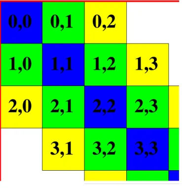
A picture illustrating the structure of the Hamiltonian is shown in Fig. 2.2. The structure

is given by the action of the operators in the Hamiltonian on the quasiparticle number. The

terms in the Hamiltonian are grouped into blocks that create and annihilate a definite number of

quasiparticles. The terms in the {0, 0}-block create and destroy zero quasiparticles. For a system

with a unique groundstate the {0, 0}-block is just a single constant, namely the groundstate

0,0

2,0 2,1 1,1

3,1 3,2 3,3 1,0

2,2 0,1

1,2 0,2

1,3 2,3

Fig. 2.2: Block-structure of the Hamiltonian. Here, the case of a Hamiltonian changing the quasiparticle number by at most 2 is shown.

energy. Operators that create quasiparticles out of the vacuum belong to {n, 0}-blocks. In Fig. 2.2 a Hamiltonian is sketched that changes the number of quasiparticles by at most 2. The one-particle dispersion is given by operators in the {1, 1}-block, interactions of two particles are in the {2, 2}-block, and so on.

Note that the illustration in Fig. 2.2 should be viewed as a scheme organizing the structure of the Hamiltonian rather than a large matrix. For example, the terms belonging to the {1, 1}- block do not only act on one-particle states. They annihilate the vacuum, but they do not annihilate states with more than one particle. Therefore, they have to be taken into account when diagonalizing the two-particle sector. This is evident in the formalism of second quantization.

It is just restated here to avoid confusion in the presentation of the quasiparticle structure of the Hamiltonian.

The quasiparticle concept is also important for the solution of the effective Hamiltonian H

. The operator H

commutes with Q. It is diagonal up to subspaces with fixed quasiparticle number. For a non-degenerate ground state the {0, 0}-block is just the energy of the groundstate.

Generally, the derivation of H

has turned the original problem into a few-body problem. This

has to be contrasted with the many-body problem one usually starts with. The n-particle sector

can be solved within this subspace handling only n particles. It is much easier to deal with

a two-particle problem than to deal with a many-body problem, even though the two-particle

interaction becomes complicated.

All observables of interest have to be transformed with the same transformation. At the end of the flow, the observables do not conserve the particle number in general. They create or destroy particles in the system. The action of the observables can be classified according to the change of the number of quasiparticles [30, 47, 48]. At zero temperature one has to consider only those operators which do not annihilate the ground state. Also the calculation of spectral quantities like spectral densities and spectral weights can be classified according to the number of quasiparticles involved.

The CUT using the MKU generator reformulates the Hamiltonian in the effective quasiparticle description. The computational effort to describe many-particle subspaces increases drastically with the particle number. The reason is that the number of terms that have to be taken into account increases. Typically, the sectors with low numbers of quasiparticles can be described with sufficient accuracy. These are the zero-, one- and two-particle subspaces. Also higher subspaces can be treated [49], however only with increasing efforts. The quasiparticle picture is most appropriate if the system can be described by the sectors with low quasiparticle numbers.

For a certain observable under study it can be checked how much of the physics is contained in the n-particle sector. As the observable is classified according to its action on the number of quasiparticles one can calculate the n-particle spectral weights. If a large part of the total spectral weight is contained in the lowest sectors the effective picture is appropriate. It describes the physics of the system under study. Sum rules can be used to check how much of the total weight is described by a certain quasiparticle sector. In actual calculations it is advisable to use sum rules to check the quality of the applied quasiparticle picture.

A particular property of MKU flow equations is that they sort the eigenvalues in ascending order of the quasiparticle number of the corresponding eigenvector [12, 13]. The quasiparticle number is measured with the counting operator Q. The example presented in the next section illustrates this fact. This property of MKU flows can lead to convergence problems. If the initial Hamiltonian has a sequence of multi-particle continua that are not ordered energetically with respect to the number of quasiparticles it can be impossible to reorganize the Hilbert space such that the energy levels are sorted according to the eigenvalues of Q. This issue will have to be discussed in the applications that are treated in the following chapters.

2.2.3. Example: Two-level problem

In this section the two-level problem is considered using CUTs. It is intended to illustrate some

of the concepts discussed so far. It also shows the difference between the MKU and Wegner

generator. The discussion of the two-level problem with a slightly different focus can also be

found in Ref. [31].

The two-level problem in the language of a system with a single spin 1/2 reads H

= E1

− ω

2 σ

+ a

2 σ

(2.2.12a)

= E −

a

2

E +

!

. (2.2.12b)

Here, the σ

are the Pauli matrices. The model contains an absolute energy constant E. The level spacing is ω. The size of the off-diagonal term is given by a. The CUT is now used to eliminate the off-diagonal term and thus to diagonalize the Hamilton.

MKU generator

For the MKU approach the counting operator is chosen to be Q = (1 − σ

)/2 = 0 0

0 1

!

. (2.2.13)

The first state is the quasiparticle vacuum since it has quasiparticle number q

= 0. For the second state, the number of quasiparticles is q

= 1. Thus, the MKU generator reads

η

(l) = sgn (q

− q

) H

(l) = − a(l)

2 iσ

= 0 −

a(l)

2

0

!

. (2.2.14)

From

∂H(l)

∂l = [η(l), H(l)] = − a(l)

2 σ

− ω(l)a(l)

2 σ

(2.2.15)

one reads the flow equations by comparing the coefficients on the left- and right-hand side. The flow equations close. They read

∂

E(l) = 0 (2.2.16a)

∂

ω(l) = a(l)

(2.2.16b)

∂

a(l) = −ω(l)a(l). (2.2.16c) The right-hand side of the flow equation is bilinear. The equations are solved by observing that a(l)

+ ω(l)

is a conserved quantity. Since convergence is proven for finite matrices we know that a(∞) = 0 and therefore

ω

= ω(∞) = p

ω(0)

+ a(0)

. (2.2.17)

The eigenstate with q

= 0 has energy E − ω

/2 and the eigenstate with q

= 1 has energy E + ω

/2. Solving the differential equation explicitly yields the l-dependence of the coefficients ω(l) and a(l). The solution reads

ω(l) = ω(∞) tanh

ω(∞)l + arctanh ω(0)

ω(∞)

, (2.2.18)

a(l) = sgn(a(0))ω(∞) s

1 − tanh

ω(∞)l + arctanh ω(0)

ω(∞)

, (2.2.19)

where sgn is the sign-function. The explicit solution confirms the exponential decay of the off-diagonal element a(l) for large values of the flow parameter.

Wegner’s generator

The problem can also be solved using Wegner’s generator. The diagonal part is H

= E1

−

σ

and thus the generator reads

η

= − a(l)ω(l)

2 iσ

. (2.2.20)

The flow equations read

∂

E(l) = 0 (2.2.21a)

∂

ω(l) = w(l)a(l)

(2.2.21b)

∂

a(l) = −ω(l)

a(l). (2.2.21c) They are cubic in the coefficients. Again, a(l)

+ ω(l)

is a conserved quantity. The Wegner flow equations are the same as the MKU flow equations up to a rescaling by ω(l). Therefore, one finds for the effective Hamiltonian

ω

= ω(∞) = sgn(ω(0)) p

w(0)

+ a(0)

. (2.2.22) Comparison

Both approaches solve the problem. However, the sorting property of η

leads to a different sequence of the eigenstates for negative values of ω(0). In the MKU solution, the first state with q

= 0 has energy E − ω

/2 and the state with q

= 1 has energy E + ω

/2. The eigenvalues are sorted according to the quasiparticle number. The value of ω(∞) is always positive.

In the Wegner approach ω(∞) has the same sign as ω(0). The eigenvalues are not sorted. The off-diagonal term a(l) is a monotonic decaying function as the right-hand side of Eq. (2.2.21c) has always the opposite sign of a(l).

On the contrary, the behavior of a(l) in the MKU approach can be non-monotonic. This is the case if ω(0) is negative. Then, the energies are in the wrong order according to the quasiparticle number of the states. The coefficients a(l) and ω(l) in the MKU-scheme are shown in Fig. 2.3 for various values of ω(0). For all values of ω(0) the coefficient a(l) approaches zero for large values of the flow parameter. The flow equations converge.

A monotonic decrease of a(l) is found for positive ω(0). If ω(0) is negative the off-diagonal term displays non-monotonic behavior. The coefficient a(l) has a maximum. The value of the maximum increases with increasing modulus ω(0). The eigenvalues are sorted according to the quasiparticle number. As long as ω(l) ≤ 0 the value of a(l) increases. As soon as ω(l) is positive the correct order of levels is reached. Then, the off-diagonal term becomes smaller.

In more general many-body problems this behavior is also found. The reordering of energies

according to their quasiparticle number will make the transformation more difficult or will even

0 0.5 1 1.5 2

a( l )

ω(0)=1.0 ω(0)=0.5 ω(0)=-0.5 ω(0)=-1.0

0 2 4

l -1

0 1 2

ω ( l )

ω(0)=1.0 ω(0)=0.5 ω(0)=-0.5 ω(0)=-1.0

Fig. 2.3: Evolution of a(l) and ω(l) in the flow for the MKU generator. The parameters are a(0) = 1 and ω(0) ∈ {1, 0.5, −0.5, −1}. Non-monotonic behavior of a(l) is found for negative values of ω(0).

For ω(0) ≤ 0 the maximal value of the off-diagonal element a(l) increases with decreasing ω(0). The maximum of a(l) is at the l-value for which ω(l) changes sign.

hinder the transformation from converging. Non-monotonic behavior of the off-diagonal part of the Hamiltonian is found. All applications that are discussed in the following chapters are not exactly solvable. The Hamiltonian has to be truncated. In this situation special attention has to be paid to possible non-monotonic behavior of the off-diagonal elements because increasing off-diagonal elements imply increasing truncation errors. Therefore, this issue will show up again in the sections were applications of the CUT are described.

2.3. Self-similar CUTs in real space

Up to now the flow equations and generators have been described in a very general fashion. The

flow equation, Eq. (2.1.2), is written down as a formal expression. We have not discussed so

far the question how to calculate and solve the flow equations. The present section will further

specify the method used in this thesis. It deals with the construction of the flow equation of

the self-similar CUT in real space. As has been mentioned before, the flow equations generally

do not produce a closed set of equations. A truncation scheme is introduced to make the CUT

approach amenable for a numerical solution. The transformation of the Hamiltonian and the

observables is described.

2.3.1. Physical motivation

Before we turn to the question how to set up the flow equations let us discuss the physical motivation for the local approach used in this thesis. The starting point of the method is a Hamiltonian formulated on a lattice. For the method to be applicable this Hamiltonian has to consist of local terms only. Infinite or long range interactions are beyond the applicability of the present treatment. In solid state physics local Hamiltonians are of great importance. A wide range of physical problems is formulated using localized Wannier states and local Hamiltonians in second quantization [1].

Note that local Hamiltonians do not necessarily describe local physics. An obvious example is a tight-binding Hamiltonian for non-interacting fermions that contains only hoppings to a few nearest neighbors. Although the Hamiltonian is very local the eigenstates are extended momentum eigenstates. If one includes interaction terms in the Hamiltonian a rich variety of phenomena are described by local Hamiltonians.

The first main concept of the present approach is to transform the Hamiltonian at hand into an effective Hamiltonian using local terms. This is done using the method of CUTs. They are a formal procedure to derive an effective Hamiltonian. The effective Hamiltonian given by the CUT is supposed to be closer to diagonality and thus easier to treat than the original problem.

The effective Hamiltonian will contain additional terms. The local approach assumes that it is possible to encode the problem truthfully in rather local terms. It is implemented as a real-space CUT. Operators are denoted in real space and the truncation scheme is based on the locality of the terms.

The second central concept is the description of the system in terms of quasiparticles. The choice of the quasiparticles depends on the physical situation. The counting operator of the quasiparticles defines the MKU generator, see also Sec. 2.2.2. The quasiparticle description gives a clear physical picture of the transformation and the effective Hamiltonian. The advantages of the quasiparticle picture inherent to the MKU-CUT has already been described in the preceding section. The local approach is combined in a natural way with the quasiparticle picture. In addition, the quasiparticle structure of terms allows a deeper analysis of the effects and of the relevance of local terms.

In contrast to a perturbative CUT a self-similar strategy is adopted here. The terms that are included in the Hamiltonian have to be chosen using definite rules. In the self-similar CUT this is done using the structure of the operators. After the new terms have been included in the Hamiltonian the CUT represents a transformation within these terms. This motivates the naming “self-similar”. The differential equation given by the CUT represents flow equations for the coefficients of the Hamiltonian. This results in a non-perturbative dependence of the effective coefficients on the system parameters.

This local approach is promising under the following circumstances. The effective model has

to incorporate the physics into local operators. The physically relevant processes have to be of

a certain range only. This is the case for small correlation lengths. For a diverging correlation

length, e. g. at a continuous phase transition, one has to be aware of a possible breakdown of

the transformation. The mapping might not be possible. This is signalled by a non-convergent behavior of the flow equation.

The local approach is particularly suited in physical situations with strong correlations. This is the type of problem where also strong-coupling expansions around the atomic limit are applied.

The reasoning behind the strong-coupling expansion also suggests the use of the local CUT approach. If the most important terms are local correlations then an expansion using terms that include these processes is promising. A prominent model describing the physics of local correlations is the Hubbard model. At large coupling and half filling it describes insulating systems with short correlation lengths. We will apply the real-space CUT to the fermionic as well as to the bosonic Hubbard model in Chap. 3 and Chap. 5, respectively. Another application are spin liquids. These are spin models that display a gap between the groundstate and the first excited states. Spin liquids are realized by local spin Hamiltonians under certain conditions.

Due to the presence of a gap the correlation length is typically of the order of only a few lattice spacings. The treatment of the spin ladder and the dimerized spin chain is presented in Chap. 4.

These systems are spin liquids for appropriate choices of the coupling constants.

The formal properties and the implementation of the real space approach to self-similar CUTs are discussed in the following.

2.3.2. Setup of the flow equations

This section presents the implementation of the CUT approach. The central formula is the flow equation for the Hamiltonian. It is restated here

∂H(l)

∂l = [η(l), H(l)]. (2.3.23)

The initial condition for this equation is the original Hamiltonian H(0) = H. The first step is the calculation of the commutator on the right-hand side. It will contain terms that are present in the original Hamiltonian and new terms. In most cases the number of newly generated terms proliferates. The flow equations do not close.

The proliferating number of terms has to be dealt with. The importance of the newly generated terms has to be judged in a certain way. Then, more important terms are kept and the others are discarded. One way to do this is to arrange the terms in perturbative order. An expansion parameter is assigned to the non-diagonal part of the Hamiltonian. Each term is of a certain order in this expansion parameter. Terms are kept up to a certain order. The resulting effective Hamiltonian contains coefficients that are given as a power series in the expansion parameter.

This strategy has been successful, see e. g. Refs. [13, 26, 27, 29, 30, 50].

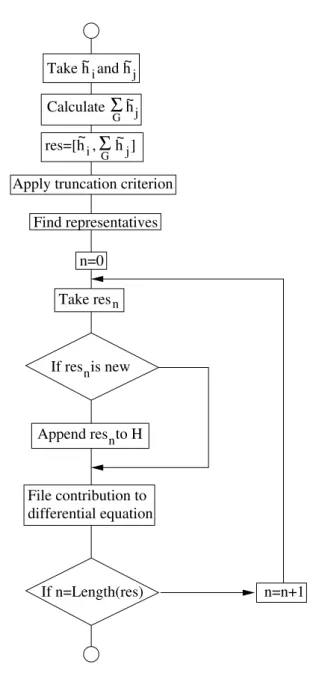
In contrast to this perturbative strategy we follow the self-similar setup of the CUT. As has been motivated in the preceding section the locality of a term is a measure for its importance if the correlation length is small. Terms are kept according to a truncation rule that implements this idea. The commutator on the right-hand side of the flow equation is computed explicitly.

The terms meeting the truncation criterion are included in the Hamiltonian. The flow equation

constitutes a differential equation for the prefactors of the terms. The example of the two-level problem treated in Sec. 2.2.3 was our first application of self-similar CUTs.

The real-space implementation of the CUTs uses the locality of operators as the main trun- cation criterion. Therefore, a measure for the locality of an operator has to be defined. An indispensable prerequisite is a physically meaningful and in particular unique way to denote the operators. We define a sort of normal-ordering of the operator products

. The normal-ordering will take place with respect to a reference ensemble. If this ensemble is unique it is a single reference state. If it consists of many states it is a reference ensemble.

First, we discuss the situation of a single reference state. It is constructed using a local reference state. The choice of this local reference state has to be motivated physically. The reference state is the state with no excitation present. Deviations from the reference state represent excitations. The full reference state is constructed as

|refi = Y

i

|0i

, (2.3.24)

where |0i

denotes the local reference state on site i. The case of a reference ensemble is encountered if there are several local states that have no excitation present. This situation will be further treated in Chap. 3. The above definition of the reference state is then generalized to the following expression for the reference ensemble

ˆ ρ

:= Y

i

1 N

X

α∈ref

|αi

hα|

!

, (2.3.25)

where the sum extends over all local states that have no quasiparticle excitation present. Their number is N

.

A product of n local operators o

· ... · o

is normal-ordered if any expectation value for m ∈ {1, ..., n}

ho

i

:= Tr(o

ρ ˆ

) (2.3.26) with the reference ensemble vanishes. Here, α

labels the local operators. Local deviations from the reference ensemble are excitations. The normal-ordered notation as defined by Eq. (2.3.26) assures that operators really deal with those excitations. The creation and annihilation operators of the excitations and products of these operators constitute the algebra of local operators.

2.3.3. Formulation with local operators

This section introduces the operator algebra for a finite local Hilbert space for the case of a single reference state. This formalism is directly applicable to the spin-systems treated in Chap. 4 and for the bosonic Hubbard system in Chap. 5. In Chap. 3 the case of a reference ensemble is encountered. The minor modifications to treat this case are discussed in Chap. 3.2.1.

1We use the expression “normal-ordering” while we are aware that we are in general not dealing with conventional normal-ordering. The applications of the method will not treat non-interacting fermions or bosons. Normal- ordering in the context of the present work refers to the standardized procedure to represent operators.

For illustration, we treat here a local Hilbert space of four states. The formalism is generalized straightforwardly to any finite number of states. Chapters 4 and 5 will also use a local basis with four states. Thus, for the sake of concreteness this dimension of the Hilbert space is used.

The four states are labeled |ni

where n ∈ {0, 1, 2, 3}. The local operators can be denoted as 4x4 matrices. Next, we construct the basis for the local operator algebra. The state |0i is defined to be the local reference state. The full reference state is the product state

|refi = Y

i

|0i

. (2.3.27)

A local operator is normal ordered if

ho

i

= h0|o

|0i

= 0.

(2.3.28)

The creation operators of local excitations have the following matrix representations

e

=











0 0 0 0

1 0 0 0

0 0 0 0

0 0 0 0











i

, (2.3.29a)

e

=











0 0 0 0

0 0 0 0

1 0 0 0

0 0 0 0











i

, (2.3.29b)

e

=











0 0 0 0

0 0 0 0

0 0 0 0

1 0 0 0











i

, (2.3.29c)

where the basis consists of the states |ni

with n ∈ {0, 1, 2, 3}. They create local excitations with flavor α ∈ {1, 2, 3}. The annihilation operators e

are the hermitian conjugates of Eq. (2.3.29).

The operators e

correspond to creation operators of hard-core particles. The application of a creation operator annihilates any singly occupied states. The operators in Eq. (2.3.29) fulfill the commutation relations of hard-core particles

h

e

, e

i

= δ

δ

− e

e

− δ

X

γ

(e

e

)

!

. (2.3.30)

Here, we have assumed that operators on different sites fulfill bosonic commutation relations.

Fermionic operators anti-commute on different sites. Compared to the usual commutation re-

lations of non-interacting particles the above equation contains additional contributions. This

complicates analytical calculations with hard-core operators. For example, a usual Bogoliubov

transformation to diagonalize a bilinear Hamiltonian is not possible for hard-core particles. The

Bogoliubov transform conserves the commutation relations of non-interacting bosons but not the one for hard-core particles.

Using the operators in Eq. (2.3.29) one can construct nine additional operators of the type

e

e

(2.3.31)

where α and β are ∈ {1, 2, 3}. Together with the creation and annihilation operators, e

and e

, this gives fifteen local operators. They are all normal ordered since the expectation value h0|o

|0i

vanishes, see Eq. (2.3.26).

The addition of the local four-dimensional identity-matrix Id(4) makes this set of operators a basis of the operators of the local Hilbert space. Any local operator o

can be decomposed into a linear combination of the basis

n

Id(4), e

, e

, e

e

α, β ∈ {1, 2, 3} o

. (2.3.32)

The role played by this basis becomes clear if one notes that the following operator is not included in the operator basis











1 0 0 0

0 0 0 0

0 0 0 0

0 0 0 0











i

. (2.3.33)

The reason is that the expectation value in Eq. (2.3.26) does not vanish. This operator projects onto the reference state, i. e. it does not deal with the excitations defined by Eq. (2.3.29).

If the operator (2.3.33) appears in the calculation it has to be rewritten in the normal-ordered form











1 0 0 0

0 0 0 0

0 0 0 0

0 0 0 0











i

= Id(4)

−











0 0 0 0

0 1 0 0

0 0 0 0

0 0 0 0











i

−











0 0 0 0

0 0 0 0

0 0 1 0

0 0 0 0











i

−











0 0 0 0

0 0 0 0

0 0 0 0

0 0 0 1











i

= Id(4)

− e

e

− e

e

− e

e

. (2.3.34) The local operators are labeled with a site index when they are used to write down the Hamil- tonian. Consequently, also products of local normal-ordered operators belonging to different sites are normal-ordered. The expectation value with respect to the reference ensemble of each separate factor vanishes.

Terms acting on several sites are composed of the local operator basis in Eq. (2.3.32). As the

operator basis is normal-ordered it is clear that all operators apart from the identity deal with

quasiparticles. As usual in second quantization, the identity operator is dropped when writing

down products of local operators. Then, the distance between the remaining normal-ordered

local operators is a measure for the locality of the induced process. This is further explained in

the next section.

e e

y x

o o o

i ^i,α

i+ e ,γ y

i+ e ,β x

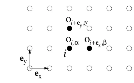
Fig. 2.4: The operator in Eq. (2.3.35) on a square lattice. Filled sites are affected by the term.

2.3.4. Transformation of the Hamiltonian

The previous section defined a physically motivated unique way to denote operators. This is necessary to implement reasonable truncation rules for the real-space CUT. The motivation to use the locality of terms for the truncation scheme has been given in Sec. 2.3. Here, we describe how this concept is implemented in a CUT calculation as a criterion for the terms that are kept in the Hamiltonian.

The Hamiltonian is a sum of products that are composed of local operators. Also products of normal-ordered operators are normal-ordered. The prefactor of a product of local operators will be called the coefficient of this term.

On the basis of the normal-ordering and of the induced standardized notation we define a measure for the locality of a term, namely its extension d. Consider the following example in two dimensions

X

i

o

o

o

. (2.3.35) Local operators are denoted by o

. In this notation i is the site index and α labels the various local operators. The local operators are normal-ordered. The above term is illustrated in Fig. 2.4. It contains operators that act on three different sites. They are depicted as filled circles in Fig. 2.4. These sites will be called the cluster belonging to this term. On all other sites the term acts as the identity. The Hamiltonian is translationally invariant because the term is summed over the index i.

The maximal taxi cab distance

d of two sites in this cluster is the extension of this term. This definition of the extension is applicable in any dimension. In particular, in one dimension the

2The taxi cab distance of two points is the minimal number of bonds on the square lattice that connect these two points.