Using different Pitman-closeness techniques for the linear combination of multivariate forecasts
Thomas Wenzel
Department of Statistics, University of Dortmund, Vogelpothsweg 87, D-44221 Dortmund, Germany
Abstract: We specify the Pitman-closeness criterion for the evaluation of multivariate forecasts in three categories. This is done closely to the definition of covariance adjustment techniques analysed in other articles. We also apply the Pitman-closeness techniques to an example dealing with German economic data.
Key words: Pitman-closeness, multivariate forecasting methods, covariance adjustment.
Acknowledgement: This work was supported by the Deutsche Forschungsgemeinschaft, Sonderforschungsbereich 475.
AMS 1991 Subject Classification: 62H12.
1 Introduction
We introduced the Pitman-closeness criterion for the evaluation of multivariate forecasts (see Wenzel, 1998b) and derived optimal weight matrices for the combination of forecasts.
There we used real valued square matrices as weights, which is the most general case and is
called Strong Pitman-closeness. Now we also analyse the situation where the weight
matrices are assumed to be diagonal as well as the case where the weights for the
combination of the multivariate forecasts are restricted to be scalar. For this we define the
notions of Medium Pitman-closeness and the Weak Pitman-closeness. The denotations
Strong, Medium and Weak Pitman-closeness are close to those of the covariance
adjustment techniques presented by Troschke (1999a). Finally we calculate the different
combinations of forecasts for a German macro economic data set.
2 The Pitman-closeness criterion
First we give a description of the problem as in Wenzel (1998b).
Assume that
( ) ′
= Y
1,..., Y
k:
Y is a random vector to be forecasted (k≥2),
( ) ′
=
1i ki i: F ,..., F
F are unbiased multivariate forecasts (i=1,...,n) for Y and )
F Y ,..., F Y (
:
1 1i k kii
= − − ′
u is the error vector of the i-th forecast method, where u : u
1,..., u
n~ N
n⋅k( ) 0 , Σ
′
′ ′
= , Σ p . d . , and there exists a vector u
i, without loss of generality u
i= u
n,so that Cov [ ( (
1 n) , , (
n 1 n) ) ]
′ ′
′ −
− u u
−u
u
Kis p.d.
Furthermore we are again giving the definition of the component-by-component Pitman- closeness.
Definition 1. The forecast F is component-by-component Pitman-closer to a random
1vector Y than the forecast F
2( F
1≠ F
2) if and only if
( Y F Y F ) 0 . 5 j { 1 ,..., k } , where F F .
P
j−
j1<
j−
j2> ∀ ∈
j1≠
j2The probability statement of Definition 1 is equivalent to
( u u ) 0 . 5 j { 1 ,..., k } , where F F .
P
j1<
j2> ∀ ∈
j1≠
j2In the following we specify the calculation procedure of optimal weights in three categories.
2.1 Strong Pitman-closeness
Here, the multivariate combination of forecasts are given as
∑
==
n1 i
i i
A
A F
F and ∑
=
=
n1 i
i i
B
B F
F , where
∈
=
) i ( )
i (
) i (
k 1 )
i ( 11 i
a a
:
L M O M
L
A IR
k×kand ∈
=
) i ( )
i (
) i (
k 1 )
i ( 11 i
b b
:
L M O M
L
B IR
k×kare matrices of weights,
Using the definitions of Wenzel (1998b), where
( )
rs r,s 1,...,n:= Σ =
Σ
, Σ
rs: = Cov ( u
r, u
s) ,
, 1 n , , 1 s , r ,: rs nn rn ns
rs =Σ +Σ −Σ −Σ = K −
V
( )
,:= Vrs r,s=1,K,n−1 V
(
nn in)
jji e
w = Σ −Σ
and therefore w
ji′ : = e
j′ ( Σ −
nnΣ
ni) , j=1,..,k, i=1,..,n−1,
′
′ ′
=
j1 j,n−1j
: w , , w
w
K,
we get the following theorem.
Theorem 1. The Strongly Pitman-closest combination (component-by-component Pitman- closest combination) of n multivariate forecasts for a random vector Y of dimension k (k≥2) is given by the matrix of weights:
] ,
[ ] ,
, [
: 1opt,str optn ,str 1 k 1 *k
opt,str
I V W I V W A
A
A = K = ′ − − ′ −
where W : = ( w
1,
K, w
k) ∼ (n−1)⋅k× k,
[ , , ] ~ ( n 1 ) k k
:
k k*
k
= I I ′ − ⋅ ×
I
K.
Proof: See Wenzel (1998b).
2.2 Medium Pitman-closeness
Here we use the restriction of diagonal matrices of weights, so
∈
=
) i ( kk )
i ( 11 i
a 0
0 a
:
OA IR
k×kand ∈
=
) i ( kk )
i ( 11 i
b 0
0 b
:
OB IR
k×kare the matrices of weights,
i=1,...,n, and ∑
= n
=
1 i
k
i
I
A , ∑
= n
=
1 i
k
i
I
B .
Using again the component-by-component Pitman-closeness definition we get the next
theorem.
Theorem 2. The Medium Pitman-closest combination (where the matrices of weights are restricted to be diagonal matrices) of n multivariate forecasts for a random vector Y of dimension k (k≥2) is given by the matrices of weights:
=
med , opt ), i ( kk med
, opt ), i ( 11 med , opt i
a 0
0 a
O
A , i=1,...,n,
where
a(jji),opt,medis the i-th component of the vector 1 1
1
1 j 1 j
−
−
′Σ
Σ (j=1,...,k) and
Σjdenotes the
covariance matrix of the individual forecast errors of the j-th component and 1 = ( 1 ,..., 1 ) ′ is a vector of length n.
Proof: The proof is straightforward. Calculating the optimal weights for the j-th component is equivalent to calculating the optimal univariate combination for this component, which is described in Wenzel (1998a).
2.3 Weak Pitman-closeness
Here we concentrate on the combination of multivariate forecasts using scalar weights.
Thus a forecast combination is given by ∑
=
=
n1 i
i i
a
a F
F , a
i∈IR , ∑
=
=
n
1 i
i
1
a . Obvious we cannot use the definition of component-by-component Pitman-closeness to calculate optimal weights for the combination. Therefore we define the Weak Pitman-closeness.
Definition 2. The forecast F is weakly Pitman-closer to the random vector Y than the
1forecast F
2( F
1≠ F
2) if and only if
. 5 . 0 F Y F
Y P
k
1 j
2 j j k
1 j
1 j
j
>
∑ − < ∑ −
=
=
The probability statement of Definition 2 is equivalent to . 5 . 0 u
u P
k
1 j
2 j k
1 j
1
j
>
∑ < ∑
=
=
Theorem 3. The Weakly Pitman-closest combination (where the weights are restricted to be scalar) of n multivariate forecasts for a random vector Y of dimension k (k≥2) is given by the vector of weights:
1 1
a
11
sum 1 weak sum
, opt n weak , opt 1 weak ,
opt
( a ,..., a )
−−
= ′
= ′
Σ
Σ , where
(
r,s)
r,s 1,...,n sum~ : = ~ 1 ′ Σ 1
=Σ and ~ 1
denotes the vector ( 1 ,..., 1 ) ′ of length k.
Proof: If we compare two forecast combinations we have to find the vector a so that for any vector b ( and b 1 )
n
1 i
∑
i=
=
≠ b
a the inequality
5 . 0 u
b u
a P
k
1 j
n
1 i
ji i k
1 j
n
1 i
ji
i
>
∑∑ < ∑∑
= =
= =
⇔ 0 . 5
u u
u
u u
u u
u u
u u
u P
kn n
2 n 1
1 k 21
11
kn n
2 n 1
1 k 21
11
>
+ + +
+ + +
< ′
+ + +
+ + +
′
K M
K K
M K
b
a holds.
The covariance matrix of the vector with the sums of the
uji’sis Σ
sumand therefore, using the conclusions as in Wenzel (1998a) we get the optimal weight vector given in the statement above.
2.4 Remarks
Consulting the paper of Troschke (1999a) we can see that the Strongly and Medium
Pitman-closest combinations are equivalent to the combinations resulting by the
corresponding covariance adjustment techniques. Therefore we use the same denotations,
which are Strong Pitman-closeness and Medium Pitman-closeness. The Weakly Pitman-
closest combination differs from the result of the weak covariance adjustment technique
because of the problem of defining a closeness criterion for this case. We have to remark
that Weak Pitman-closeness is a criterion using the absolute of the sum of errors, which is
not really reasonable for the comparison of forecasts. Obviously, the Strongly Pitman-
closest combination is component-by-component Pitman-closer to Y than the Medium
Pitman-closest combination and the Weakly Pitman-closest combination and likewise the
Medium Pitman-closest combination is component-by-component Pitman-closer to Y than
the Weakly Pitman-closest combination.
3 Analysing German economic data
Klapper (1998) investigated German macro economic data and analysed different univariate combination techniques. In another article he also used a multivariate rank approach for the combination of the individual forecasts (Klapper, 1999). We derived the Pitman-closest combinations for this problem where we assumed that the errors are normally distributed with zero mean. Using only a ten years history for estimating the covariance matrix (by the usual ML-estimator) we have the problem of a singular matrix V.
In the calculation of the Strongly Pitman-closest combination we therefore use the Moore- Penrose-Inverse V
+instead of V
−1but then the result depends on which of the individual forecasts is defined as F . The order of the other forecasts does not influence the result. A
ncomprehensive discussion of this can be found in Troschke (1999b).
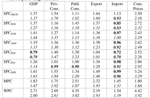
In the following table we present the Root Mean Square Errors (RMSE) and the Mean Absolute Deviations (MAD) of the special combinations relative to the RMSE and the MAD of the simple average of the individual forecasts.
Table 1: RMSE and MAD of the special combinations relative to the RMSE and MAD of the simple average forecast.
GDP Priv.
Cons.
Publ.
Cons.
Export Import Cons.
Prices SPCOECD 1.37
1.37
1.54 1.70
1.11 1.02
1.64 1.60
1.13 0.93
2.50 2.16 SPCWSI 1.37
1.27
1.16 1.16
1.43 1.18
1.37 1.31
0.85 0.83
2.72 2.32 SPCSVR 1.41
1.44
1.27 1.35
1.14 1.13
1.36 1.38
0.97 1.00
2.43 2.29 SPCAWF 1.19
1.15
1.36 1.30
1.36 1.12
1.38 1.23
0.96 0.92
2.62 2.49 SPCIFW 0.79
0.79
1.40 1.47
1.30 1.23
1.04 1.01
0.72 0.70
2.52 2.26 SPCIFO 1.26
1.14
1.01 0.99
1.00 0.90
1.36 1.28
0.98 0.91
2.86 2.92 SPCDIW 1.61
1.61
1.55 1.84
1.34 1.20
1.49 1.46
0.99 0.96
3.24 3.29
MPC 1.83
1.47
1.75 1.92
2.51 1.87
2.32 1.95
1.45 1.31
1.80 1.68
WPC 2.71
2.00
2.69 2.61
4.35 3.02
2.19 1.93
1.54 1.39
4.42 3.92