Evaluation of economic forecasts for Austria

https://doi.org/10.1007/s00181-019-01814-1

Evaluation of economic forecasts for Austria

Ines Fortin

· Sebastian P. Koch

· Klaus Weyerstrass

Received: 5 July 2018 / Accepted: 4 December 2019

© The Author(s) 2019

Abstract

In this paper, we evaluate macroeconomic forecasts for Austria and analyze the effects of external assumptions on forecast errors. We consider the growth rates of real GDP and the demand components as well as the inflation rate and the unemployment rate.

The analyses are based on univariate measures like RMSE and Theil’s inequality coefficient and also on the Mahalanobis distance, a multivariate measure that takes the variances of and the correlations between the variables into account. We compare fore- casts generated by the two leading Austrian economic research institutes, the Institute for Advanced Studies (IHS) and the Austrian Institute of Economic Research (WIFO), and additionally consider the forecasts produced by the European Commission. The results indicate that there are no systematic differences between the forecasts of the two Austrian institutes, neither for the traditional measures nor for the Mahalanobis distance. Generally, forecasts become more accurate with a decreasing forecast hori- zon, as expected; they are unbiased for forecast horizons of less than a year considering traditional measures and for the shortest forecast horizon considering the Mahalanobis distance. Finally, we find that mistakes in external assumptions, in particular regarding EU GDP and the oil price, translate into forecast errors for GDP and inflation.

Keywords Forecast evaluation · MAE · RMSE · Theil’s U2 · Mean directional accuracy · Mahalanobis distance · External assumptions · Small open economy · Austria

JEL Classification C53 · E37 · E66

Electronic supplementary material The online version of this article (https://doi.org/10.1007/s00181- 019-01814-1) contains supplementary material, which is available to authorized users.

B

Extended author information available on the last page of the article

1 Introduction

Macroeconomic forecasts provide important information for economic policy mak- ers, companies and private households. In Austria, two research institutes, the Institute for Advanced Studies (Institut für Höhere Studien, IHS) and the Austrian Institute of Economic Research (Wirtschaftsforschungsinstitut, WIFO), have a long tradition of providing economic forecasts. In addition, the Austrian National Bank (Oesterreichis- che Nationalbank, OeNB) as well as some private banks publishes macroeconomic forecasts for Austria. Further, international institutions like the European Com- mission (EC), the International Monetary Fund (IMF), and the Organisation for Economic Cooperation and Development (OECD) periodically produce forecasts for Austria.

This paper focuses on the evaluation of IHS and WIFO forecasts, because they share certain features that make them particularly suitable for comparison. First, both institutes publish their forecasts always and exactly at the same time in a joint press conference. This implies that the information sets for both institutes are very similar, as they use roughly the same cutoff day until which information is taken into account.

The period between the cutoff day and the publication day is, at around one week, rather short, unlike for OeNB and international institutions (OECD, IMF, EC), which are part of a forecasting system that includes a large number of countries. The longer this interval, the more likely it is that recent events cannot be incorporated in the newest forecast publication. Both IHS and WIFO produce four short-term forecasts per year, which are published toward the end of each quarter. OeNB, on the other hand, publishes macroeconomic forecasts twice a year, in June and December.

Second, the target variables of IHS and WIFO are exactly the same. One might assume that this is true for all forecasts, but as practitioners know, there is a wide range of possible choices regarding the exact specification of the variable in question.

On a quarterly basis the forecaster can, for example, choose whether to include a sea- sonal adjustment, a working-day adjustment, or the irregular component. Regarding the growth rates of GDP and its demand components, both IHS and WIFO forecast annual averages of the original series, i.e., not adjusted for working days. This might be true also for the private banks, but it is not for OeNB. The OeNB forecasts are part of the Eurosystem forecasts, which are based on series adjusted for working days to facilitate a better comparison across the different European countries. Different series are also available when it comes to inflation and unemployment. The national inflation rate usually differs only slightly from the harmonized European rate. How- ever, this is not true for the unemployment rate due to substantial methodological differences.

Third, the objectives and therefore the evaluation and the underlying loss func- tions are the same for IHS and WIFO. Both institutes aim at producing “exact” point forecasts. Apart from definitional issues about what “exact” means, producing exact forecasts is not always the main goal of forecasters. It may well be, for example, that internal macroeconomic forecasts of a finance ministry should instead produce a con- servative GDP forecast in order to reduce bad surprises when it comes to tax receipts.

Overly pessimistic (and sometimes optimistic) forecasts, for their part, might increase

the forecaster’s media coverage and thus enhance its public visibility.

In any case, we assume that the main objective of both IHS and WIFO is to generate “exact” point forecasts, i.e., forecasts with the smallest forecast error.

Yet the precise definition of forecast error is far from obvious. On the one hand, there are different “realized” values with which the forecasts can be compared. We take as realizations the first release of the annual national accounts published by the Austrian statistical office (Statistik Austria) around nine months after the end of the year. Inflation and unemployment figures are usually not subject to revision. On the other hand, the choice of the loss function with respect to the forecasting error could alter the determination of the “best” forecast.

Traditionally, measures of accuracy like the mean absolute error (MAE), the mean absolute percentage error (MAPE), the mean-squared error (MSE), the root-mean- squared error (RMSE), the mean directional accuracy (MDA), and Theil’s inequality measure U2 have been used. Although these measures are widely accepted and regu- larly applied in forecast evaluations, they have the drawback of being one-dimensional;

i.e., they examine each variable separately and do not take the relationship between different forecasts into account. Therefore, we additionally consider the Mahalanobis distance, which assesses jointly the forecasts of a group of variables.

This multi- dimensional measure takes both the (potentially different) variances of the variables and the correlations between the different variables into account. In addition, we test for the unbiasedness of the forecasts and for differences between the forecasters.

Specifically, we evaluate the growth forecasts of GDP and its demand components:

private consumption, gross fixed capital formation, exports, and imports. We also consider the forecasts of unemployment and inflation. The forecast assessment is based on the four forecasts published per year for the current year and the following year.

Furthermore, we consider forecasts of the European Commission, where we point out that a direct comparison with the national forecasts by IHS and WIFO may be flawed due to the different sets of information available at the time of forecasting. We examine the EC spring and autumn forecasts for the current year and the following year, published in May and November. The related analysis excludes inflation and unemployment, since national and international forecasters use different definitions.

Finally, we complement our forecast evaluation with an analysis of the effects of errors regarding external assumptions on forecast errors for GDP and inflation.

For this purpose, we consider a number of assumptions related to the international environment, including the GDP growth of the European Union, the oil price, and the foreign exchange rate (euro versus US dollar) and examine whether and to what

1 Obviously, both IHS and WIFO are also interested in public visibility, but not at the cost of producing

“extreme” (false) forecasts.

2 Alternative objectives might be to predict business-cycle turning points. See, for example, Giusto and Piger (2017) and Kovacs et al. (2017).

3 Sinclair and Stekler (2013) were probably the first to use the Mahalanobis distance in the context of macroeconomic forecasting, when they compared different vintages of US GDP and major component estimates. Other applications of this method in forecast evaluation include Sinclair et al. (2012,2015), Döhrn (2015) and Sinclair et al. (2016).

extent mistakes in these assumptions translate into forecast errors for GDP growth and inflation.

Economic forecasts for Austria have been evaluated before. Baumgartner (2002a) compared IHS and WIFO forecasts; Baumgartner (2002b) examined the differences between national forecasts (IHS, WIFO) and OECD forecasts; Ragacs and Schneider (2007) investigated national (IHS, WIFO, OeNB) and international (EC, IMF, OECD) forecasts; and Schuster (2018) studied national (IHS, WIFO, OeNB) and international (EC, IMF, OECD) forecasts.

The paper is structured as follows. The next section sketches the dataset. We then describe the traditional evaluation measures and the Mahalanobis distance. In the following section we present and discuss the results, including the findings related to the effects of external assumptions on the forecast error. Finally, we summarize the main findings and conclude.

2 Data

The data include IHS and WIFO economic forecasts published in the period 1995 to 2017. In each year, the two institutes publish four forecasts, usually at the end of each quarter, i.e., in March, June, September, and December. At each forecast date and for each forecast variable, annual forecasts for the years t and t + 1 are published.

Hence, the included forecast years cover the period 1995 to 2017, and for each year eight forecasts are available, four published in the year t − 1 (year-ahead forecasts), and four published in the year t (current-year forecasts). For the first year, 1995, only four forecasts are available, as the t +1 forecasts of 1994 are missing.

We consider the following variables: annual growth rates of real GDP, private consumption, real gross fixed capital formation (investment), exports, and imports. In addition to these demand components, forecasts of the inflation rate as measured by the national consumer price index and forecasts of the unemployment rate (according to national statistics, i.e., registered unemployment) are evaluated.

As actual data, we use the first (and usually final) publications of annual inflation and annual unemployment data; for the national accounts variables, we take the first release of the annual accounts, published by the Austrian statistical office approximately nine months after the end of a given year. While there are almost no revisions of unemployment and inflation rates, GDP and its components are frequently revised, and these revisions are sometimes large relative to the absolute values of the growth rates. This issue is particularly relevant for capital formation, due to its large variability.

We use the first release of the annual accounts rather than the first “preliminary” release based on quarterly accounts, which are available three months after the end of the year, as the annual accounts are based on a larger information set. In a robustness check, we find that the differences between these data vintages are very small (see Sect. 4.3).

Alternatively, it would be possible to take the latest data release.

4 However, the underlying models might run on a shorter periodicity.

5 Note that neither IHS nor WIFO published a forecast in June 1997 and hence the Junetforecasts for 1997 and the Junet−1 forecasts for 1998 are missing.

The question of what values to take as realizations or actual values is a much debated issue. In the literature on forecast evaluations, both first and later data vin- tages (releases) have been used as benchmarks. Sinclair et al. (2016) evaluate German macroeconomic forecasts for the year 2013, published around December 2012. They compare these forecasts with the first release of actual data for 2013, published in Jan- uary 2014, as well as the “final” (second) release of February 2014. The corresponding results are very similar. Sinclair and Stekler (2013) compare different vintages of US GDP and its ten major components: namely, the initial estimates available one month after the end of the quarter, and the estimates available three months after the end of the quarter. Despite the existence of some biases, overall the differences are rather small.

Kirby et al. (2015) look at the accuracy of the NIERS’s forecasts of GDP growth in the UK, the USA, and the euro area, comparing these forecasts to the first release of the variables. Sheng (2015) evaluates real GDP growth, inflation, and unemployment forecasts of members of the FOMC of the US Federal Reserve System, using “final”

estimates that are released roughly three months after the end of the quarter. Chen et al.

(2016) evaluate forecasts of GDP growth and inflation for ten Asian countries, where forecasts are compared to initial releases. As a robustness check, they use revised data and find that the results are rather similar. The European Commission, in its regular forecast assessments,

uses different realized values for current-year and year-ahead forecasts. The realizations are taken from the same publication as the forecasts, i.e., from the autumn publications for year-ahead forecasts and from the spring publica- tions for current-year forecasts. Evaluations of macroeconomic forecasts for Austria usually take the first preliminary release of the national accounts provided by WIFO.

Baumgartner (2002a, b) considers additionally the first “final” release produced by the Austrian statistical office, as do we, and concludes that the differences are very small.

3 Evaluation measures

The selection of appropriate measures for the evaluation of forecasts is not straight- forward. Obviously, the “best” economic forecast is a forecast that accurately predicts the realization of the forecast variable. Equally obviously, it is almost impossible to deliver “exact” predictions. Therefore, intervals, e.g., the 68% confidence interval, are sometimes published. In business-cycle research, the correct anticipation of so-called turning points is even more important than the exact forecast of a certain GDP growth rate. A standard evaluation criterion is that the forecast beats the naive no-change fore- cast. Furthermore, the forecasts should be unbiased, implying that the forecast should not be systematically too optimistic or too pessimistic. We evaluate the accuracy of the IHS and WIFO forecasts on the basis of traditional one-dimensional and more novel multi-dimensional measures.

6 The first study is Keereman (1999); the most recent evaluation is Fioramanti et al. (2016).

7 These studies include Baumgartner (2002a,b), Ragacs and Schneider (2007), and Schuster (2018) 8 We also find that the differences between using the first preliminary release and the first official release are very minor (see Sect.4.3).

3.1 Traditional measures

We apply the following traditional measures: the mean absolute error (MAE)

, the root-mean-squared error (RMSE)

, the mean absolute percentage error (MAPE)

, Theil’s inequality coefficient (U2)

, and the mean directional accuracy (MDA)

. The RMSE is defined as the square root of the average difference between the forecast and the actual realization. Since it is scale dependent, the RMSE is useful for a compari- son between different forecasts, but its magnitude is not meaningful in itself. Theil’s inequality coefficient (see Theil 1966) compares a given model-generated forecast with the naive forecast of no change. If the forecast is better than the naive no-change assumption, then U2 is smaller than one.

The test for unbiasedness of the forecast is based on a procedure introduced by Mincer and Zarnowitz (1969). The test rests on regressing the realized values on a constant and the forecast. However, as Sinclair et al. (2010) point out, forecast errors might depend on the state of the economy, e.g., the stage of the business cycle.

Therefore, these authors suggest to include a dummy for the state of the economy.

This gives rise to estimating Eq. (1).

A

= α + β F

+ γ D

+

(1) where F

and A

are the forecast for and the actual value at year t, respectively. D

is the recession dummy, which is not present in the original version of the test. The recession dummy takes the value 1 if the economy is in a recession, and 0 otherwise. In order to identify the stage of the business cycle, first a simple Hodrick–Prescott (HP) filter is applied to the level of GDP over the entire data sample, and then the output gap is calculated as the deviation of actual GDP from the HP trend. We define a recession as a year with a negative output gap.

For the forecast to be unbiased, α should not be significantly different from zero, β should not significantly deviate from one, and γ should not be significantly different from zero. We test this joint hypothesis with a Wald test. For the growth rates of GDP and the demand components, we employ both the original Mincer–Zarnowitz test, i.e., without the recession dummy, and the

9 M AE=¹_nn

t=1|Ft−At| 10 R M S E=

1 n

n

t=1(Ft−At)² 11 M A P E=_n¹n

t=1^Ft−AAt ^t

12U2=

n

t=h+1(F_t−A_t)² _n

t=h+1(^At−At−h)² 13 M D A=_n−1¹ n

t=21(sgn(At−A_t−1)=sgn(Ft−F_t−1))

whereFtandAtare the forecast for and the actual value att, respectively, andhis the forecast horizon (h=1 for current-year forecasts andh=2 for year-ahead forecasts). Note that in the definition of the mean directional accuracy we do not consider the values of zero separately but together with the values of ones. We thus conclude that the forecast direction of a given variable is assessed correctly if either the forecast goes down when the actual value goes down, or if the forecast goes up or stays the same when the actual value goes up or stays the same.

14 Note that for GDP and the demand components the assumption of no change refers to the growth rates of these variables.

15 Strictly speaking, this is a downturn rather than a recession.

modified version that includes this dummy. However, we believe that for the inflation rate and the unemployment rate, only the original test is meaningful: the labor market lags behind real economic activity. Hence, in general, unemployment does not rise at the same time as GDP growth falls (it may even be negative), but only later on, sometimes even only when real activity has already risen again. Furthermore, the labor market in Austria, as in many other European countries, is characterized by labor hoarding: companies react to an economic downturn only to an attenuated extent so as to avoid hiring costs in the following recovery. Inflation, likewise, does not follow the economic cycle very closely; hence, there are periods which according to our simple definition would be classified as a recession, but that also involve high and persistent inflation. At the same time, defining the recession dummy for each variable separately would also not be very meaningful, since a recession is usually characterized as a significant and widespread decline in activity across the economy lasting longer than a few months.

In addition, we apply the encompassing test introduced by Chong and Hendry (1986) in order to judge whether one institute’s forecast contains all the information inherent in the other institute’s forecast:

F E

= α

+ β

F

+

, F E

= α

+ β

F

+

(2) where F E

= F

− A

, i = IHS, WIFO, is the forecast error for year t. The null hypothesis is that all information included in one forecast is already contained in the other forecast and hence β

= 0 or β

= 0. In the general version of the test, one given forecast is compared with a number of other forecasts, and the idea is that if a single forecast contains all the information contained in the other individual forecasts, that forecast will be just as good as a combination of all other forecasts.

3.2 The Mahalanobis distance

The aforementioned measures share the drawback of being one-dimensional. There- fore, we also apply the Mahalanobis distance, which is a multi-dimensional evaluation measure taking the variances of and the correlations between the variables into account.

This measure allocates weights to the individual forecast errors, which are implied by the variance–covariance matrix of the variables. In utilizing this methodology, we follow Sinclair and Stekler (2013).

In order to formally define the Mahalanobis distance, let us assume that F

is an m-dimensional vector of forecasts for time period t, and A

is an m-dimensional vector of actual realizations of a variable at time period t . Let m be the number of variables to be predicted. If, for example, the growth rates of GDP, the inflation rates, and the unemployment rates are taken into account, m equals three.

F

=

⎛

⎜ ⎝ F

...

F

⎞

⎟ ⎠ , A

=

⎛

⎜ ⎝ A

...

A

⎞

⎟ ⎠ (3)

Let F ¯ and A ¯ be the mean column vectors of F

and A

, respectively, and let W be the pooled sample variance-covariance matrix of F

and A

. Then we define the Mahalanobis distance, M , as

M = F ¯ − ¯ A

W

F ¯ − ¯ A

(4) Under the assumptions of normality, one can construct an F -statistic based on the squared Mahalanobis distance, M

, to test the null hypothesis that two sets of forecasts have the same population means.

We employ this test in order to examine the difference between the IHS and WIFO joint forecasting accuracies.

For assessing the unbiasedness of the joint forecasts, or rather the existence of any systematic errors, we follow the procedure used by Sinclair and Stekler (2013).

This is a more general approach than investigating the variables separately (as done in Sect. 3.1). According to this approach, a given forecast error should not depend on past forecast errors of either the variable itself or other variables. We thus construct a first-order vector autoregression (VAR(1)) of the forecast errors of each variable, which is given by

F E

= β

+ β

F E

+

(5) where F E

is an m-dimensional vector of forecast errors at time t (with F E

= F

− A

), β

is an m−dimensional vector of constants, and β

is an m × m matrix of coefficients on the lags of the forecast error. If the joint estimators are unbiased, then none of the coefficients in the VAR should be significant: the constant estimates should be zero, the coefficients on the own lags should be zero, and none of the past errors made in forecasting the other variables should Granger-cause any of the other errors.

This implies a total number of m × 3 single hypotheses that need to be examined. Instead of testing each null hypothesis separately at a given level α, we use the Bonferroni–Holm test (see Holm 1979). This is a multiple-level α test, whereby the probability of committing any type I error is always smaller than or equal to a given level α .

In contrast to our procedure, Sinclair and Stekler (2013) examine the null hypotheses separately and do not employ multiple-level α tests.

4 Results

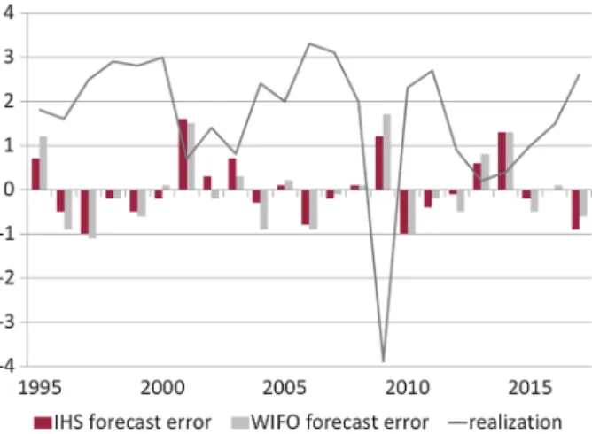
Both IHS and WIFO forecasts of GDP growth show a smoothing pattern over the busi- ness cycle. While in upturns both institutes tend to underestimate growth, in downturns they both overestimate growth. The pattern is shown in Fig. 1, which plots the forecast

16 F= _(nⁿ¹₁ⁿ_+n²⁽ⁿ_2)m(n¹⁺ⁿ²₁^−m−1)_+n2−2)M², withmandn1+n2−m−1 the degrees of freedom, wheren1andn2 are the numbers of observations of the first and second group of variables (see McLachlan 1999).

17 This is a generalization of the Holden and Peel (1990) test for bias.

18 Testing each null hypothesis at the significance levelαmay lead to an inflated occurrence of multiple type I errors producing spurious significance. For more details on multiple-levelαtests, see, for example, Hochberg and Tamhane (1987), Hsu (1996) and Alt et al. (2011).

Fig. 1 Forecast biases and realizations of GDP growth. The figure shows the forecast errors (forecasts minus realized values) of IHS and WIFO Marchtforecasts and the realized values of GDP growth

errors of the current-year March forecasts against the realized values. This smoothing behavior seems to be characteristic of economic forecasters,

as unexpected shocks (“extreme” events) are not highly predictable in general.

Another observation is that the forecast disagreement concerning GDP growth across the two institutes, measured in terms of the absolute difference between the respective forecasts, seems to be larger in downturns than in upswings. This is reflected by a negative correlation between the forecast differences and the realized values, for all current-year forecasts of GDP.

This pattern suggests that forecasters particularly disagree in the assessment of economic downturns or recessions.

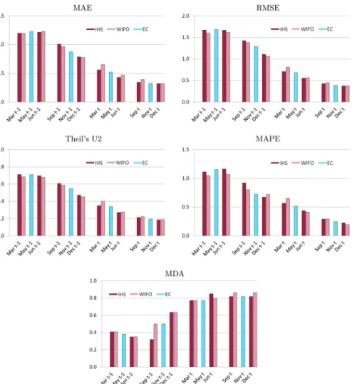
4.1 Traditional measures 4.1.1 Accuracy

Tables 1 and 2 report the forecast evaluation results based on the traditional measures.

Table 1 presents the values of the respective test statistics, while Table 2 assesses the improvement of the forecasts over time. For the latter, the evaluation measure for a given forecast horizon is divided by the “best” evaluation measure, no matter whether this best measure is provided by IHS or WIFO. Usually the best forecast is the one with the shortest forecast horizon (i.e., the December t forecast). Also, better forecasts usually go along with smaller values of the evaluation measures, except for the mean directional accuracy (MDA), where larger values imply better forecasts. The best forecast for a given variable thus shows a value of one. A value of two, for example,

19 See, for example, Ragacs and Schneider (2007), Sinclair et al. (2010), Sinclair and Stekler (2013), and An et al. (2018).

20 The correlation is equal to−0.6 for the average of the four current-year forecasts, and it is significant at the 5% level (p=0.0027).

Table1Evaluationresults:MAE,RMSE,Theil’sU2,MAPE,MDA GDPConsump.Invest.ExportsImportsInflationUnempl. IHSWIFOIHSWIFOIHSWIFOIHSWIFOIHSWIFOIHSWIFOIHSWIFO MAE Mart-11.201.200.740.683.012.814.003.893.723.910.730.670.720.64 Junt-11.211.230.760.732.862.714.074.123.773.930.650.650.620.62 Sept-11.010.970.730.652.702.533.513.543.293.430.680.620.460.47 Dect-10.790.770.660.602.362.053.123.062.952.950.540.530.390.38 Mart0.560.650.640.622.032.182.592.792.783.060.370.370.300.24 Junt0.430.470.600.571.802.022.122.202.412.520.170.180.140.15 Sept0.340.390.440.441.341.262.092.202.012.130.110.100.050.06 Dect0.320.320.430.391.281.241.912.001.871.860.020.040.030.03 RMSE Mart-11.671.610.920.853.813.556.015.765.595.530.870.830.870.78 Junt-11.661.620.940.893.693.465.895.925.505.540.830.830.780.73 Sept-11.431.380.880.793.453.195.335.195.064.940.820.750.580.58 Dect-11.111.060.800.732.932.514.294.404.154.330.620.630.470.45 Mart0.710.810.800.762.512.573.323.733.533.930.450.430.360.30 Junt0.550.560.750.712.192.382.772.843.083.090.220.210.180.18 Sept0.430.450.590.591.701.702.642.692.552.700.140.130.090.08 Dect0.370.380.570.521.641.582.362.452.322.450.050.060.050.06 Theil’sU2 Mart-10.710.680.810.740.620.580.720.690.710.700.690.661.040.93 Junt-10.700.680.810.770.590.550.690.690.680.690.640.640.910.85 Sept-10.610.590.770.700.560.520.630.620.640.630.650.600.690.69 Dect-10.470.450.700.640.480.410.510.520.530.550.500.500.560.54

Table1continued GDPConsump.Invest.ExportsImportsInflationUnempl. IHSWIFOIHSWIFOIHSWIFOIHSWIFOIHSWIFOIHSWIFOIHSWIFO Mart0.350.400.700.670.410.420.400.440.450.500.350.340.430.36 Junt0.270.270.640.610.350.380.320.330.380.380.170.170.220.21 Sept0.210.220.520.520.280.280.310.320.320.340.110.100.110.10 Dect0.190.190.500.460.270.260.280.290.290.310.040.050.060.07 MAPE Mart-1111.2104.9103.895.6261.6203.2125.9119.8257.7269.355.153.710.19.0 Junt-1116.3106.7108.5100.6263.8236.3129.2127.6269.2285.551.754.68.78.8 Sept-192.180.4100.683.1226.0220.197.298.1201.6214.153.948.36.46.7 Dect-167.372.285.480.2181.5208.484.084.6159.6188.839.836.65.45.4 Mart57.065.376.176.4158.4252.274.175.3171.0190.824.522.04.23.5 Junt44.041.266.360.9189.8304.964.558.7154.2133.810.910.82.02.1 Sept29.229.641.344.4183.5180.253.256.894.493.67.05.80.70.9 Dect22.719.542.138.0185.0227.646.145.876.973.70.92.60.40.5 MDA Mart-10.410.410.550.550.500.590.230.360.360.550.450.550.550.55 Junt-10.350.350.400.400.450.450.350.350.350.400.550.450.650.70 Sept-10.320.500.450.550.550.640.410.500.410.410.500.590.770.73 Dect-10.640.640.550.640.730.820.500.590.410.360.860.770.730.73 Mart0.770.770.820.730.770.820.640.730.550.730.910.820.730.77 Junt0.850.800.750.700.850.850.750.750.600.650.950.950.950.90 Sept0.820.860.730.730.860.860.770.770.640.820.950.951.000.95 Dect0.820.860.770.770.910.820.770.770.730.731.001.001.001.00 Thetableshowstheunivariateevaluationresultsforallforecastvariables,fortheeightforecastspublishedbyIHSandWIFO

Table2Improvementofforecastsovertime:univariatemeasures GDPConsumpt.Invest.ExportsImportsInflationUnempl. IHSWIFOIHSWIFOIHSWIFOIHSWIFOIHSWIFOIHSWIFOIHSWIFO MAE Mart-13.733.721.921.762.432.272.102.042.002.1033.4031.0027.6724.67 Junt-13.773.831.961.882.312.192.132.162.032.1130.1129.9023.8723.87 Sept-13.143.001.881.672.182.041.841.851.771.8531.2028.6017.6718.00 Dect-12.452.411.711.561.911.661.631.601.581.5925.0024.6014.8314.50 Mart1.742.031.651.611.641.761.361.461.501.6417.2016.8011.509.33 Junt1.331.461.541.471.451.631.111.151.301.357.958.365.405.58 Sept1.071.221.131.151.081.021.091.151.081.145.204.602.002.33 Dect1.001.001.101.001.031.001.001.051.001.001.001.801.001.33 RMSE Mart-14.464.291.771.622.422.252.552.442.412.3918.6417.8416.9815.24 Junt-14.454.321.801.712.342.192.502.512.372.3917.7617.8215.2314.28 Sept-13.813.681.691.522.182.022.262.202.192.1317.5216.1611.3311.31 Dect-12.972.841.541.391.851.591.821.871.791.8713.3913.509.178.88 Mart1.892.161.531.451.591.631.411.581.521.709.579.257.015.94 Junt1.481.501.441.371.391.511.171.201.331.334.714.573.573.44 Sept1.151.211.131.141.081.071.121.141.101.163.032.791.731.63 Dect1.001.011.101.001.041.001.001.041.001.061.001.341.001.15 Theil’sU2 Mart-13.833.681.771.622.422.252.552.442.412.3918.6417.8417.8316.00 Junt-13.763.651.761.672.292.142.442.452.322.3417.3717.4315.6414.67 Sept-13.273.161.691.522.182.022.262.202.192.1317.5216.1611.8911.88 Dect-12.552.441.541.391.851.591.821.871.791.8713.3913.509.639.32

Table2continued GDPConsumpt.Invest.ExportsImportsInflationUnempl. IHSWIFOIHSWIFOIHSWIFOIHSWIFOIHSWIFOIHSWIFOIHSWIFO Mart1.892.161.531.451.591.631.411.581.521.709.579.257.366.24 Junt1.461.481.401.341.361.481.151.181.301.304.604.473.713.53 Sept1.151.211.131.141.081.071.121.141.101.163.032.791.851.71 Dect1.001.011.101.001.041.001.001.041.001.061.001.341.001.21 MAPE Mart-15.705.382.732.521.651.282.752.613.503.6658.1956.7525.7223.07 Junt-15.965.472.862.651.671.492.822.783.663.8854.5957.7022.2422.43 Sept-14.724.122.652.191.431.392.122.142.742.9156.9251.0616.3917.04 Dect-13.453.702.252.111.151.321.831.852.172.5642.0738.7013.8613.71 Mart2.923.352.002.011.001.591.621.642.322.5925.9323.2710.818.91 Junt2.252.111.741.601.201.931.411.282.091.8211.5311.395.155.27 Sept1.501.521.091.171.161.141.161.241.281.277.366.101.842.26 Dect1.161.001.111.001.171.441.011.001.041.001.002.771.001.34 MDA Mart-10.470.470.670.670.550.650.290.470.440.670.450.550.550.55 Junt-10.410.410.490.490.500.500.450.450.430.490.550.450.650.70 Sept-10.370.580.560.670.600.700.530.650.500.500.500.590.770.73 Dect-10.740.740.670.780.800.900.650.760.500.440.860.770.730.73 Mart0.890.891.000.890.850.900.820.940.670.890.910.820.730.77 Junt0.980.930.920.860.940.940.970.970.730.790.950.950.950.90 Sept0.951.000.890.890.950.951.001.000.781.000.950.951.000.95 Dect0.951.000.940.941.000.901.001.000.890.891.001.001.001.00 Thenumberforagivenforecastvariableandagivenevaluationcriterionistheratiowithrespecttotheminimumcriterion(ofeitherIHSorWIFO)forthatvariable

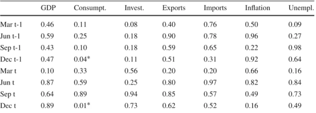
Table 3 Diebold–Mariano test for difference in accuracy

GDP Consumpt. Invest. Exports Imports Inflation Unempl.

Mar t-1 0.46 0.11 0.08 0.40 0.76 0.50 0.09

Jun t-1 0.59 0.25 0.18 0.90 0.78 0.96 0.27

Sep t-1 0.43 0.10 0.18 0.59 0.65 0.22 0.98

Dec t-1 0.47 0.04^∗ 0.11 0.51 0.31 0.92 0.64

Mar t 0.10 0.33 0.56 0.20 0.20 0.66 0.16

Jun t 0.87 0.59 0.25 0.80 0.97 0.82 0.84

Sep t 0.64 0.89 0.94 0.85 0.57 0.49 0.73

Dec t 0.89 0.01^∗ 0.73 0.62 0.52 0.16 0.49

The table listspvalues for testing the null hypothesis that IHS and WIFO forecasts show the same accuracy, where the loss function is the squared forecast error. Starred figures indicate that the null hypothesis is rejected at the 5% significance level and hence that IHS and WIFO forecasts show different levels of accuracy

means that the respective forecast error is twice the error of the best forecast for the respective variable.

In order to judge whether the forecasts across the two institutes differ significantly from each other, we employ a standard Diebold–Mariano test. For basically all vari- ables and all forecast horizons, our results imply that the forecasts of IHS and WIFO do not differ significantly from each other. The only exception is consumption growth in the December year-ahead and current-year forecasts, where, as shown in Table 3, WIFO seems to provide a marginally better forecast (involving a smaller forecast error).

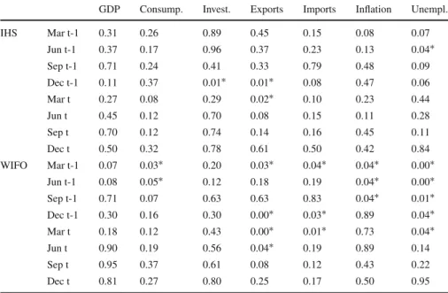
Another way of comparing the forecasts is to perform an encompassing test, which tells us whether the forecast of one institute could be improved by using the other institute’s forecast. The results, presented in Table 4, show that mostly the forecast of one institute indeed encompasses the forecast of the other institute. In particular, this is always true for GDP forecasts. In addition, all current-year IHS forecasts (with one exception) encompass the respective WIFO forecasts. In total, the IHS forecast does not encompass the WIFO forecast in four out of 56 cases, while the WIFO forecast does not encompass the IHS forecast in 17 out of 56 cases.

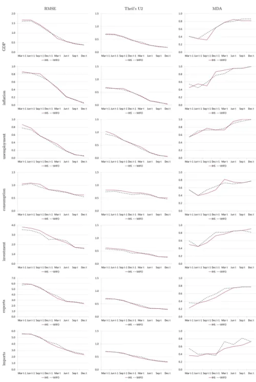
More important than the small differences between the forecasts is the common feature that all forecasts improve considerably over time (see Fig. 2 and Tables 1 and 2). This improvement is most distinct for the inflation rate and the unemployment rate, where the forecast errors are almost zero in September and December of the current year t . This result is to be expected, since inflation and unemployment data are published monthly, in a very timely fashion, and in the December forecast almost all of the realizations are known.

21 These conclusions rely on the Diebold–Mariano test using the squared forecast error as the loss function.

If we take the absolute forecast error we do not find any difference at all between the two institutes when it comes to forecast accuracy.

Table 4 Encompassing test

GDP Consump. Invest. Exports Imports Inflation Unempl.

IHS Mar t-1 0.31 0.26 0.89 0.45 0.15 0.08 0.07

Jun t-1 0.37 0.17 0.96 0.37 0.23 0.13 0.04^∗

Sep t-1 0.71 0.24 0.41 0.33 0.79 0.48 0.09

Dec t-1 0.11 0.37 0.01^∗ 0.01^∗ 0.08 0.47 0.06

Mar t 0.27 0.08 0.29 0.02^∗ 0.10 0.23 0.44

Jun t 0.45 0.12 0.70 0.08 0.15 0.11 0.28

Sep t 0.70 0.12 0.74 0.14 0.16 0.45 0.11

Dec t 0.50 0.32 0.78 0.61 0.50 0.42 0.84

WIFO Mar t-1 0.07 0.03^∗ 0.20 0.03^∗ 0.04^∗ 0.04^∗ 0.00^∗

Jun t-1 0.08 0.05^∗ 0.12 0.18 0.19 0.04^∗ 0.00^∗

Sep t-1 0.71 0.07 0.63 0.63 0.83 0.04^∗ 0.01^∗

Dec t-1 0.30 0.16 0.30 0.00^∗ 0.03^∗ 0.89 0.04^∗

Mar t 0.18 0.12 0.43 0.00^∗ 0.01^∗ 0.73 0.04^∗

Jun t 0.90 0.19 0.56 0.04^∗ 0.19 0.89 0.14

Sep t 0.95 0.37 0.61 0.08 0.12 0.43 0.22

Dec t 0.81 0.27 0.80 0.25 0.17 0.50 0.95

The table listspvalues for testing the null hypothesis that the IHS (and WIFO) forecast encompasses the forecast of the other institute. Starred figures indicate that the null hypothesis is rejected at the 5%

significance level and hence the other institute contributes to explaining one’s own forecast errors

Also with regard to Theil’s U2, the improvement of the forecasts over time is clearly visible. As mentioned above, in contrast to the RMSE the absolute value of Theil’s U2 is meaningful. It should be below one, since only then is the forecast better than the naive no-change assumption. Theil’s U2 is above unity only in one case:

namely the first IHS unemployment forecast. Especially for current-year forecasts, this measure is clearly below 1, particularly for the forecasts of the inflation rate and the unemployment rate, but also for the GDP growth forecast. The improvement is least distinct for the consumption growth forecast. This might be related to the fact that consumption is rather smooth over time. Hence, the growth rates do not fluctuate much over time, rendering the no-change assumption that is the benchmark of Theil’s U2 more difficult to beat.

Similarly to the other traditional measures, the difference between the two institutes with respect to getting the directional change right is rather small. Among all variables, inflation is assessed best: already at the beginning of the current year the directional change is projected correctly by IHS in more than 90% of all cases, and by WIFO in more than 80%. The directional change of GDP growth is forecast about equally well.

The directions of import changes seem to be harder to predict: considering the March

forecasts in year t , roughly 60% of all changes are anticipated correctly by IHS, and

roughly 70% by WIFO.

Fig. 2 RMSE, Theil’s U2, and MDA for decreasing forecast horizon

4.1.2 Bias

The original and the modified Mincer–Zarnowitz tests show that in general the fore- casts are neither too high nor too low (Tables 5, 6). Based on the original test, i.e., without taking the state of the business cycle into account, the growth forecasts of pri- vate consumption and exports, and the forecasts of the unemployment rate are the only ones in which the null hypothesis of no systematic forecast errors has to be rejected—

and then only in a small number of cases. If the recession dummy is included, only some consumption growth forecasts show signs of being biased. Overall, the forecast- ers of IHS and WIFO do not seem to make any systematic errors, even when the state of the economy in the business cycle is taken into account.

Summarizing all results based on traditional, one-dimensional accuracy measures, we can draw the following conclusions: (i) all forecasts improve considerably over time, which is what one would expect; (ii) the forecasts published by the two institutes IHS and WIFO do not differ significantly from each other, except in two out of 56 cases; (iii) in most cases the forecast of one institute encompasses the forecast of the other institute; and (iv) there are basically no systematic forecast errors for the forecasts published in year t, including when the state of the economy is taken into account.

4.2 The Mahalanobis distance

We assess the joint forecasts of three different groups of variables. The first group includes all variables considered (hereafter called All), i.e., growth rates of real GDP, private consumption, real gross fixed capital formation, exports, and imports, as well as the inflation rate and the unemployment rate. The second group includes real GDP growth, the inflation rate, and the unemployment rate (hereafter called Macro), and the third group includes growth rates of real GDP, real gross fixed capital formation, private consumption, exports, and imports (hereafter called Demand). Very often forecasts of the Macro group are reported to provide a quick overview of the economic outlook.

4.2.1 Accuracy

Table 7 reports the joint evaluation results of IHS and WIFO forecasts using the Maha- lanobis distance, considering all variables (All), the Macro group, and the Demand group. The differences between the two institutes are rather small. In each group the maximum difference between the two institutes is observed for the second earliest forecast, i.e., the June forecast published in year t − 1. This goes along with what one might expect: forecasts are usually more divergent the earlier they are produced.

With a decreasing forecast horizon, forecasts normally move closer to the realized

values (i.e., the forecast error decreases), and hence, the difference between the two

institutes also shrinks, as more information becomes available. Overall, this obser-

vation is borne out in Fig. 3, which plots the evaluation results for the three groups

of variables. IHS forecasts show a slightly larger joint forecast error at early forecast

dates. By contrast, both institutes show nearly identical forecast errors for the Macro

Table5Mincer–Zarnowitztestforunbiasedforecasts GDPConsumpt.Invest.ExportsImportsInflationUnempl. IHSWIFOIHSWIFOIHSWIFOIHSWIFOIHSWIFOIHSWIFOIHSWIFO Mart-10.080.180.01∗0.02∗0.170.400.070.420.060.120.03∗0.090.02∗0.02∗ Junt-10.110.180.01∗0.02∗0.200.320.310.310.240.200.080.070.03∗0.02∗ Sept-10.590.730.02∗0.050.680.610.920.860.800.960.130.410.120.04∗ Dect-10.300.560.04∗0.090.480.290.04∗0.04∗0.130.350.810.700.090.08 Mart0.420.770.04∗0.100.480.900.03∗0.03∗0.250.210.430.960.300.11 Junt0.660.960.080.210.870.970.220.080.440.420.250.980.370.25 Sept0.800.910.220.470.780.920.190.100.230.250.850.740.080.23 Dect0.670.830.370.650.590.900.090.130.070.160.330.400.690.77 Thetablelistspvaluesfortestingthenullhypothesisofnobias.Starredfiguresindicatethatthenullhypothesisofnobiasisrejectedatthe5%significancelevel

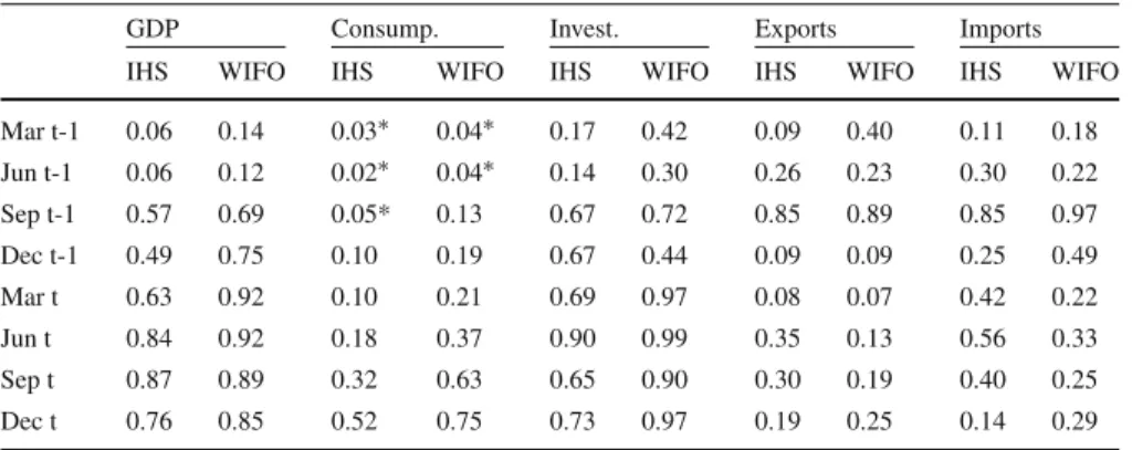
Table 6 Modified Mincer–Zarnowitz test for unbiased forecasts

GDP Consump. Invest. Exports Imports

IHS WIFO IHS WIFO IHS WIFO IHS WIFO IHS WIFO

Mar t-1 0.06 0.14 0.03^∗ 0.04^∗ 0.17 0.42 0.09 0.40 0.11 0.18

Jun t-1 0.06 0.12 0.02^∗ 0.04^∗ 0.14 0.30 0.26 0.23 0.30 0.22

Sep t-1 0.57 0.69 0.05* 0.13 0.67 0.72 0.85 0.89 0.85 0.97

Dec t-1 0.49 0.75 0.10 0.19 0.67 0.44 0.09 0.09 0.25 0.49

Mar t 0.63 0.92 0.10 0.21 0.69 0.97 0.08 0.07 0.42 0.22

Jun t 0.84 0.92 0.18 0.37 0.90 0.99 0.35 0.13 0.56 0.33

Sep t 0.87 0.89 0.32 0.63 0.65 0.90 0.30 0.19 0.40 0.25

Dec t 0.76 0.85 0.52 0.75 0.73 0.97 0.19 0.25 0.14 0.29

The table listspvalues for testing the null hypothesis of no bias, when the state in the business cycle is accounted for. Starred figures indicate that the null hypothesis is rejected at the 5% significance level

Table 7 Evaluation results: Mahalanobis distance

Mahalanobis distance Ratio with respect to minimum

All Macro Demand All Macro Demand

IHS WIFO IHS WIFO IHS WIFO IHS WIFO IHS WIFO IHS WIFO

Mar t-1 0.810 0.736 0.438 0.380 0.707 0.659 2.22 2.01 15.35 13.32 1.94 1.81 Jun t-1 0.901 0.710 0.493 0.356 0.795 0.631 2.47 1.94 17.28 12.48 2.18 1.73 Sep t-1 0.657 0.562 0.295 0.229 0.591 0.517 1.80 1.54 10.33 8.04 1.62 1.42 Dec t-1 0.586 0.504 0.191 0.221 0.532 0.482 1.60 1.38 6.71 7.74 1.46 1.32 Mar t 0.449 0.471 0.132 0.044 0.403 0.431 1.23 1.29 4.61 1.56 1.10 1.18 Jun t 0.476 0.455 0.058 0.040 0.450 0.389 1.30 1.24 2.03 1.41 1.23 1.07 Sep t 0.447 0.430 0.045 0.029 0.419 0.427 1.22 1.18 1.58 1.00 1.15 1.17 Dec t 0.480 0.365 0.039 0.038 0.479 0.365 1.31 1.00 1.36 1.32 1.31 1.00 The left panel of the table shows the Mahalanobis distance for the three different groups of variables (All, Macro,Demand) for the eight forecasts provided by IHS and WIFO. The right panel shows the ratio of that distance with respect to the minimum distance (of either IHS or WIFO) for a given group

group over the last three forecast dates. A bit surprisingly, the joint forecast errors of IHS for the group of all variables (All) and for the Demand group increase slightly from the penultimate to the last forecast, while the corresponding WIFO joint forecast errors decrease, as one would expect. Since this behavior is not visible in the univariate evaluation measures, it is probably inherent to the Mahalanobis distance, i.e., related to the covariances between the variables. For all forecast horizons, IHS and WIFO joint forecasts do not differ significantly from each other.

Likewise, based on the univariate analysis presented in Sect. 4.1.1, we have concluded that the two institutes do not provide significantly different forecasts.

22 More precisely, the null hypothesis of equal means cannot be rejected, for any given forecast horizon.

This is tested by considering the Mahalanobis distance between IHS and WIFO forecasts, for each forecast horizon (considering the impliedF-distribution), see Sect.3.2.

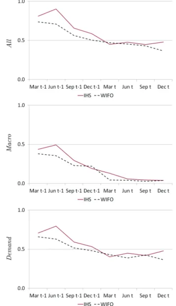
Fig. 3 Mahalanobis distance for decreasing forecast horizon. The figure shows the Mahalanobis distance for a decreasing forecast horizon for three different groups of variables (All,Macro,Demand)

The three graphs in Fig. 3 show that the joint forecasts clearly improve over time, and

this is particularly true for the Macro group. The reason is probably the relatively high

accuracy (small forecast errors) of the inflation and unemployment forecasts, already

pointed out for the univariate results, which account for two of the three variables in

that group. For the Macro group, the joint forecast errors implied by the latest forecasts

are smaller than the errors implied by the first forecasts by a factor larger than ten. For

the other two groups of variables (All and Demand), this factor is equal to or below

two, and hence, the improvement over time is less pronounced (see Table 7).

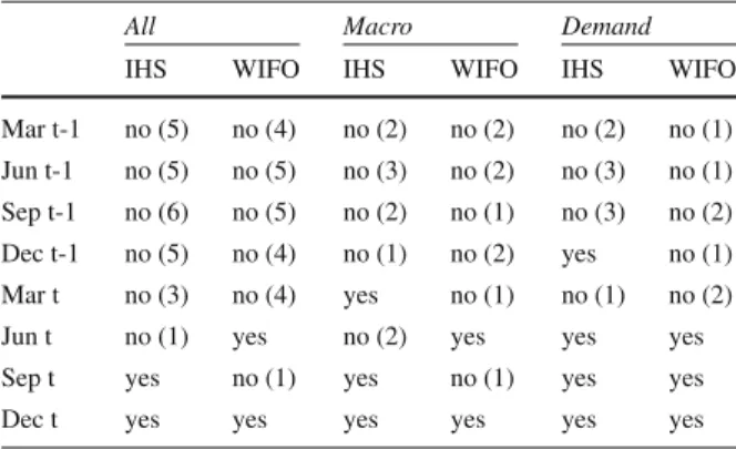
Table 8 Unbiasedness of joint

forecasts All Macro Demand

IHS WIFO IHS WIFO IHS WIFO

Mar t-1 no (5) no (4) no (2) no (2) no (2) no (1) Jun t-1 no (5) no (5) no (3) no (2) no (3) no (1) Sep t-1 no (6) no (5) no (2) no (1) no (3) no (2) Dec t-1 no (5) no (4) no (1) no (2) yes no (1) Mar t no (3) no (4) yes no (1) no (1) no (2)

Jun t no (1) yes no (2) yes yes yes

Sep t yes no (1) yes no (1) yes yes

Dec t yes yes yes yes yes yes

The results are based on the Bonferroni–Holm procedure, a simple multiple-levelαtest, at a global significance level of 5%. Figures in brackets denote the number of rejections, where the total number of individual hypotheses is equal to 21 (All), 9 (Macro), and 15 (Demand)

4.2.2 Bias

In order to examine whether joint forecasts are unbiased, a fairly large number of null hypotheses need to be tested. The concrete number (m × 3) depends on the number of variables considered in the joint forecast and is thus equal to 21, 9, and 15 in our case. Table 8 presents the results. Only for the most recent forecast, i.e., the December t forecast, are the joint forecasts unbiased for all the groups under consideration (All, Macro, Demand) for both Austrian research institutes. This means that in a VAR(1) system of the forecast errors implied by the variables under consideration, neither the constant terms nor the lagged errors are significant, and in addition none of the given errors is significantly Granger-caused by the other errors. Further, the September t forecasts are largely unbiased, and in the case of the IHS all forecasts are unbiased. If a joint forecast is not unbiased, we report the number of cases in which the null hypotheses are rejected. For all current-year forecasts, the maximum number of individual hypotheses rejected is three (IHS) or four (WIFO), out of a total of 21 cases (All).

We provide more detailed results in Tables 1 to 4 in the Online Appendix in order to be able to assess the precise source(s) of the bias. For example, the single rejection for the WIFO September t forecasts in the groups All and Macro originates from the unemployment forecast error being Granger-caused by the other forecast errors (see Tables 2 and 3 in the Online Appendix). In fact, it is nearly always true that the source of the bias can be found in a given forecast error being Granger-caused by the other forecast errors.

4.3 Robustness checks

We perform two sets of robustness checks. First, we exclude the year 2009 from our

analyses since during this year of the “Great Recession” GDP in Austria dropped by

3.8%. The declines of fixed capital formation and exports were even more severe, at

7.2% and 14.4%, respectively. No forecasts predicted this extreme economic down- turn during most of the year 2008. Second, we use another benchmark with which we compare our forecasts, namely the first estimate of annual national accounts published in March of year t + 1. We use this release only for the robustness check, and not as the benchmark, for two reasons. First, the annual accounts are based on a larger infor- mation set and are thus usually subject to smaller revisions than the first estimate of March. Second, the March release is produced by WIFO, i.e., one of the two forecasts institutes, on behalf of the Austrian statistical office, while the release published in late summer is produced by the statistical institute itself. Of course, inflation and unem- ployment figures are usually not subject to revision, unless methodological changes are implemented.

The results for both robustness checks are very similar to our main results. In partic- ular, there are no systematic deviations, and thus, the conclusions remain unaffected.

In contrast to our study, Baumgartner (2002a, b) uses the first estimate of the annual national accounts, provided by WIFO, as a benchmark. But he performs the analy- sis also with the realizations taken from the national accounts produced by Statistik Austria and finds, as we do, that there are hardly any differences in the results.

4.4 Comparison with European Commission forecasts

In this section, we compare the economic forecasts of IHS and WIFO with the forecasts for Austria made by the European Commission, which produces economic forecasts twice a year.

The EC publication dates, spring forecasts in May and autumn forecasts in November, differ from those of IHS and WIFO. As a consequence, the information available for national and international forecasters is not the same, which complicates a proper forecast comparison. If, for example, the national March issues are compared with the EC spring issues, then the EC has an information advantage and should, ceteris paribus, provide more accurate forecasts. If, on the other hand, the EC spring issues are compared with the national June issues, then IHS and WIFO have an information advantage.

If there is no systematic difference in the quality of forecasting across national and international institutions, then the forecasts should improve with a decreasing forecast horizon. Note that this section excludes inflation and unemployment from the analysis, since national and international forecasters use different definitions.

Figure 4 shows the different measures of accuracy for the national and international forecasts of GDP growth for different forecast horizons. We have twelve forecast dates in total, eight from the national institutes and four from the European Commission.

23 A few years ago the EC started to publish an additional winter forecast. The winter forecasts are not considered in our analysis due to the short time series.

24 Baumgartner (2002b) investigates the forecast accuracy of the two national institutes (IHS and WIFO) and OECD by grouping the national and international forecasts in two alternative ways (and performing the analysis twice). One grouping reflects an informational advantage for the national institutes; the other grouping an informational advantage for the international institute (OECD).

25 IHS and WIFO use the national definitions of inflation (CPI) and the unemployment rate (Claimant Count based on administrative data from the benefits system), while the EC uses harmonized measures (HICP and LFS, respectively).

Fig. 4 Measures of accuracy for different dates of forecasts and different forecasting institutions for GDP growth

As we can see from the graphs, the first three GDP growth forecasts that we con- sider, i.e., the year-ahead forecasts in March, May, and June, are roughly the same and do not clearly improve over time. Similarly, the last three forecasts, i.e., the current-year forecasts of September, November, and December, do not seem to get better over time. By contrast, the GDP growth forecasts do seem to get more accu- rate from the year-ahead forecasts in September through the current-year forecasts in September. This general observation holds more or less across all the different measures of accuracy that we evaluated. More formally, as shown in Table 9, the Diebold–Mariano test for two successive forecasts

confirms our impression. The year-ahead forecasts in September, November, and December are significantly better

26 The null hypothesis of the test states that the forecast accuracy is the same for both forecasts, while the alternative hypothesis says that the more recent forecast is more accurate. Note that this is slightly

Table 9 Diebold–Mariano test for successive national and international GDP forecasts

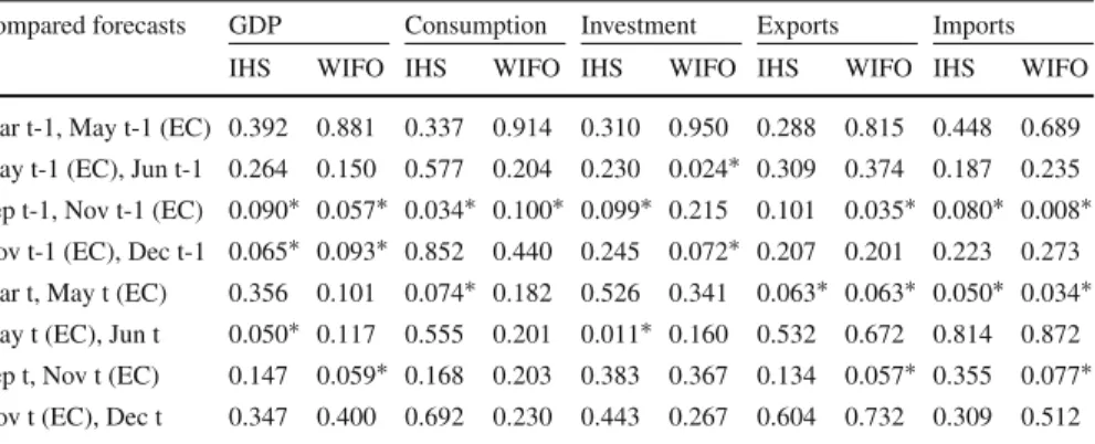
Compared forecasts GDP Consumption Investment Exports Imports

IHS WIFO IHS WIFO IHS WIFO IHS WIFO IHS WIFO

Mar t-1, May t-1 (EC) 0.392 0.881 0.337 0.914 0.310 0.950 0.288 0.815 0.448 0.689 May t-1 (EC), Jun t-1 0.264 0.150 0.577 0.204 0.230 0.024^∗ 0.309 0.374 0.187 0.235 Sep t-1, Nov t-1 (EC) 0.090^∗ 0.057^∗ 0.034^∗ 0.100^∗ 0.099^∗ 0.215 0.101 0.035^∗ 0.080^∗ 0.008^∗ Nov t-1 (EC), Dec t-1 0.065^∗ 0.093^∗ 0.852 0.440 0.245 0.072^∗ 0.207 0.201 0.223 0.273 Mar t, May t (EC) 0.356 0.101 0.074^∗ 0.182 0.526 0.341 0.063^∗ 0.063^∗ 0.050^∗ 0.034^∗ May t (EC), Jun t 0.050^∗ 0.117 0.555 0.201 0.011^∗ 0.160 0.532 0.672 0.814 0.872 Sep t, Nov t (EC) 0.147 0.059^∗ 0.168 0.203 0.383 0.367 0.134 0.057^∗ 0.355 0.077^∗ Nov t (EC), Dec t 0.347 0.400 0.692 0.230 0.443 0.267 0.604 0.732 0.309 0.512 The table listspvalues for testing the null hypothesis that successive forecasts of GDP growth show the same accuracy against the alternative hypothesis that the more recent forecast is more accurate, where the loss function is the squared forecast error. Starred figures indicate that the null hypothesis is rejected at the 10% significance level and hence that the more recent forecast is more accurate

than their preceding counterparts (for both IHS and WIFO), and the same applies for the current-year September forecast (for both IHS and WIFO), the current-year June forecast (IHS), and the current-year November forecast (against the preceding WIFO forecast).

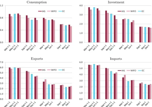
We observe a similar pattern in the quality of forecasts for the remaining vari- ables, i.e., for the growth rates of consumption, investment, exports, and imports. For those variables as well, the forecasts do not considerably improve over the period of the first forecasts (March to June year-ahead forecasts) or over that of the last fore- casts (September to December current-year forecasts), while they usually do improve over the remaining period (year-ahead September forecasts to current-year September forecasts), see Fig. 5 and Table 9.

Overall, this comparison between the IHS, WIFO, and EC forecasts corroborates our findings that the accuracy of the forecast depends much more on the time of publication, i.e., on the data available when preparing the forecast, than on the question of which institution publishes the forecast.

4.5 Effects of external assumptions

Macroeconomic forecasts are usually conditional on assumptions about the interna- tional economic environment, such as world trade, GDP growth for the main trade partners, the oil price, exchange rates, and monetary and fiscal policies. This is partic- ularly true for small open economies like Austria’s.

Forecast errors may then result from wrong external assumptions, a poor forecast model, or both. In addition, revi-

Footnote 26 continued

different from the Diebold–Mariano tests performed before, when the alternative hypothesis was that the two competing forecasts were different.

27 Note, for example, that in 2017 the external trade to GDP ratio of Austria amounted to 104%, while it was 27% in the USA.

Fig. 5 RMSE for different dates of forecasts and different forecasting institutions for the growth of con- sumption, investment, exports, and imports

sions of national accounts data may be relevant. This section investigates the effects of errors in external assumptions of this sort. Since such errors usually propagate to the forecast errors, the following question arises: To what extent can forecast errors be explained by errors involving external assumptions?

In order to answer this question, we perform a regression analysis in the spirit of Keereman (2003), Fioramanti et al. (2016), and the European Commission (2016) to determine the influence of deviations of external assumptions on the forecast error of Austrian GDP growth. We consider the effect of an unexpected change in the growth rate of GDP of the European Union, the oil price, and the foreign exchange rate. A similar set of regressions is performed for the inflation forecast for Austria, with a view to answering the question whether and to what extent mistakes in external assumptions translate into inflation forecast errors. The analyses are based on 17 to 22 observations, depending on the forecasting horizon and the institute.

Table 10 summarizes the results with respect to prediction errors in the growth rate

of GDP. We find a positive influence of EU GDP errors on the forecast error of the

Austrian GDP, which is highly significant for the first five forecasts. With regard to the

positive sign, this is what we would expect, since an overestimation of external growth

should lead to a higher than realized national growth rate. With regard to oil prices our

expectation about the sign is ambiguous. Overestimated oil prices might lead, on the

one hand, to an underestimation of growth due to overestimated import prices. On the

other hand, overestimated oil prices might just reflect the overestimation of the state of

the global economy. The latter is what almost all our results show, in particular when

the coefficients are significant. We find little evidence that mistakes in the oil price

Table 10 Effects of external assumptions on forecast errors for GDP

Coefficients Pvalues R² Obs. F-test

Const. GDP_EU Oil FX Const. GDP_EU Oil FX

IHS Mar t-1 0.05 0.83^∗ 0.02^∗ −0.04 0.753 0.000 0.006 0.14 0.92 17 51.7^∗ Jun t-1 0.09 0.88^∗ 0.02^∗−0.01 0.601 0.000 0.035 0.74 0.90 17 38.9^∗ Sep t-1 −0.03 0.89^∗ 0.02 −0.03 0.866 0.000 0.052 0.40 0.86 18 27.6^∗ Dec t-1 0.05 0.96^∗ 0.01 0.00 0.735 0.000 0.213 0.92 0.79 20 20.1^∗ Mar t −0.03 0.87^∗ 0.00 −0.02 0.801 0.001 0.976 0.50 0.50 21 5.6^∗ Jun t 0.04 0.51 0.00 0.07 0.744 0.076 0.734 0.19 0.43 20 4.0^∗ Sep t 0.00 0.53 −0.02 0.10 0.996 0.116 0.257 0.45 0.20 21 1.4 Dec t 0.01 0.57 −0.03 0.05 0.874 0.140 0.295 0.80 0.26 21 2.0 WIFO Mar t-1−0.09 0.92^∗ 0.01 0.01 0.503 0.000 0.142 0.46 0.90 22 54.3^∗

Jun t-1 −0.05 0.87^∗ 0.01 0.02 0.774 0.000 0.240 0.20 0.87 21 36.8^∗ Sep t-1 −0.02 0.87^∗ 0.01 0.01 0.915 0.000 0.147 0.63 0.82 22 27.3^∗ Dec t-1−0.04 0.95^∗ 0.01 0.01 0.804 0.000 0.222 0.64 0.74 22 17.1^∗ Mar t −0.07 1.04^∗ 0.00 0.00 0.621 0.000 0.988 0.86 0.55 22 7.4^∗ Jun t −0.04 0.38 0.00 0.08 0.747 0.256 0.874 0.14 0.39 21 3.7*

Sep t 0.01 0.50 0.02 0.03 0.958 0.224 0.242 0.67 0.24 22 1.9 Dec t −0.04 0.56 −0.03 0.07 0.649 0.152 0.202 0.65 0.24 22 1.9 The table shows the results of regressing the forecast error of the Austrian GDP growth rate on unexpected changes in the growth rate of the EU GDP, the growth rate of the oil price, and the growth rate of the foreign exchange rate (euro versus US dollar). Starred figures indicate significance at the 5% level

prediction explain GDP forecast errors and no evidence at all for unexpected changes in the exchange rate. Note that about 90% of the variation of the GDP forecast error can be explained by the deviations in the external assumptions for the first (i.e., the March t − 1) forecast. This number drops to about 50% for the fifth (i.e., the March t ) forecast. Note, in addition, that the results across the two institutes are very similar.

A robustness check which excludes the crisis year 2009 shows no major changes in the results.

Table 11 shows the corresponding results for the effect of external assumption on the inflation forecasts. As anticipated, we find that unexpected changes in the oil price do indeed explain part of the inflation forecast error. If oil prices are thought to increase more, inflation is overestimated as well, and vice versa. However, for current- year forecasts the statistical significance either disappears (IHS) or becomes weaker (WIFO). In the case of the inflation forecast errors, roughly 50% to 60% of the variation can be explained by deviations in external assumptions for the first three forecasts. By contrast, we do not find any evidence for the propagation of mistakes in the external assumptions concerning GDP growth and exchange rates. Again, a robustness check excluding the crisis year 2009 yields only very minor changes in the analysis.

While other studies

consider the effects of external assumptions only for one current-year forecast and one year-ahead forecast, this analysis provides a more

28 Keereman (2003), Fioramanti et al. (2016), and European Commission (2016).