QCD Crossover at Finite Chemical Potential from Lattice Simulations
Szabolcs Borsanyi ,1 Zoltan Fodor,1,2,3,4 Jana N. Guenther,1,5 Ruben Kara ,1Sandor D. Katz,2 Paolo Parotto ,1 Attila Pasztor,2 Claudia Ratti,6 and Kálman K. Szabó1,3
1Department of Physics, Wuppertal University, Gaussstrasse 20, D-42119 Wuppertal, Germany
2Institute for Theoretical Physics, ELTE Eötvös Loránd University, Pázmány P. s´etány 1/A, H-1117 Budapest, Hungary
3Jülich Supercomputing Centre, Forschungszentrum Jülich, D-52425 Jülich, Germany
4Physics Department, UCSD, San Diego, California 92093, USA
5University of Regensburg, Department of Physics, Regensburg D-93053, Germany
6Department of Physics, University of Houston, Houston, Texas 77204, USA
(Received 11 February 2020; revised 5 May 2020; accepted 1 July 2020; published 29 July 2020) We provide the most accurate results for the QCD transition line so far. We optimize the definition of the crossover temperatureTc, allowing for its very precise determination, and extrapolate from imaginary chemical potential up to realμB≈300 MeV. The definition ofTc adopted in this work is based on the observation that the chiral susceptibility as a function of the condensate is an almost universal curve at zero and imaginary μB. We obtain the parameters κ2¼0.0153ð18Þ and κ4¼0.00032ð67Þ as a continuum extrapolation based onNt¼10, 12, 16 lattices with physical quark masses. We also extrapolate the peak value of the chiral susceptibility and the width of the chiral transition along the crossover line. In fact, both of these are consistent with a constant function ofμB. We see no sign of criticality in the explored range.
DOI:10.1103/PhysRevLett.125.052001
Introduction.—One of the most important open problems in the study of quantum chromodynamics (QCD) at finite temperature and density is the determination of the phase diagram of the theory in the temperature (T)-baryochemical potential (μB) plane. It is now established by first principle lattice QCD calculations that the transition at μB¼0is a smooth crossover [1,2]for physical quark masses. Due to the lack of a real phase transition, the crossover temperature is of course ambiguous, since different definitions can lead to different values for it. Observables related to chiral symmetry (i.e., the chiral condensate and its susceptibility) yield a transition temperature around 155–160 MeV[3–6].
Extending our knowledge to theμB>0part of the phase diagram turns out to be very challenging due to the notorious sign problem. Since this makes direct simulation at finiteμBimpossible, the state of the art for finite density QCD on fine lattices is to use one of two extrapolation methods. The first method is the direct calculation of Taylor coefficients[7–17]using simulations atμB ¼0, while the second is to use simulations at imaginary chemical poten- tials (μ2B<0), where the sign problem is absent, and later perform an extrapolation of different quantities to a real chemical potential (μ2B>0)[18–31]. It is often conjectured
that in theðT;μBÞplane the crossover line, departing from ðTc;μB¼0Þ, eventually turns into a first-order transition line. The pointðTCEP;μCEPÞ separating the crossover and the first-order transitions is known as the critical endpoint (CEP), where the transition is expected to be of second order. Though there have been attempts in extracting information about the location of the supposed CEP from lattice simulations[15,26,32–37], these attempts face great difficulties as extrapolation-type methods have the property of giving reliable results mostly in the immediate vicinity ofμB ¼0.
In this Letter, we address the problem of calculating the Taylor coefficients of the crossover temperature around μB¼0, parameterized as follows:
TcðμBÞ
TcðμB¼0Þ¼1−κ2
μB
TcðμBÞ 2
−κ4
μB
TcðμBÞ 4
… ð1Þ
along the phenomenologically relevant strangeness neutral- ity line. In this work we improve the uncertainty on κ4
available in the literature [16] by a factor of 6, giving a state-of-the-art determination of the crossover line in the ðT;μBÞplane. In particular, as we will show, at chemical potentialsμB>200MeV, the error on theTcextrapolation is dominated by the subleading coefficients, e.g., κ4. The coefficientsκ2 andκ4can be calculated with either one of the standard extrapolation methods. A direct evaluation of the μB derivatives from μB ¼0 ensembles was used in Refs.[38,39]. The current state of the art using theμB ¼0 simulation method is Ref. [16], which includes the first Published by the American Physical Society under the terms of
the Creative Commons Attribution 4.0 International license.
Further distribution of this work must maintain attribution to the author(s) and the published article’s title, journal citation, and DOI. Funded by SCOAP3.
PHYSICAL REVIEW LETTERS 125, 052001 (2020)
continuum extrapolated results forκ4. Here we will employ an analytical continuation from imaginary μB instead and use lattices as fine asNt¼16. This is motivated by the fact that the signal-to-noise ratio of higher μB derivatives is suppressed with powers of the lattice volume; therefore the calculation of higher order derivatives requires very high statistics. Determinations ofκ2using the imagi- nary μB method with continuum extrapolation include Refs. [24,25]. Finally, in Ref. [30]the two methods were compared with a careful check of the systematics, and a very good agreement was found for the coefficientκ2. The transition line was also studied in chiral effective models, see, e.g., the recent Ref. [40].
We also study the strength of the crossover by extrapo- lating the width of the transition and the value of the chiral susceptibility at the transition to real μB in the continuum limit. While one always has to be careful not to overinterpret results from extrapolations, we currently do not see any sign of criticality up to μB≈300 MeV, as the crossover tran- sition does not get narrower or stronger in this region.
On chiral observables in the transition region.—For the lattice simulations, we use 4-stout improved staggered fermions with an aspect ratio of LT ¼4 and temporal lattice sizes of Nt¼10, 12, 16. The details of the simulation setup can be found in the Supplemental Material [41]. The use of rooted staggered fermions may come with additional systematic effects that we did not consider in this Letter. Ideally, this work should be repeated with a chiral discretization.
The main observables in this study are the renormalized dimensionless chiral condensate and susceptibility, respec- tively defined as
hψψi ¼¯ −½hψψi¯ T−hψψi¯ 0mud
f4π ; χ¼ ½χT−χ0m2ud
f4π ; with hψψ¯ iT;0¼T
V
∂logZ
∂mud
χT;0¼T V
∂2logZ
∂m2ud ; ð2Þ
where we assumed isospin symmetry, i.e., mu¼md¼ mud. In the above equations, the subscripts T, 0 indicate values at finite and zero temperature, respectively. In the following,hψψi¯ andχare always shown after applying the correction to satisfyns¼0with zero statistical error (see the Supplemental Material [41] for details). The peak height of the susceptibility is an indicator for the strength of the transition, while the peak position in temperature serves as a definition for the chiral crossover temperature. It was pointed out in Refs.[3,4]that different normalizations of the susceptibility, such as using1=f4πor1=T4to defineχ in Eq. (2), can shift the peak position by 11 MeV. This difference could be considered as a measure for the broadness of the chiral transition.
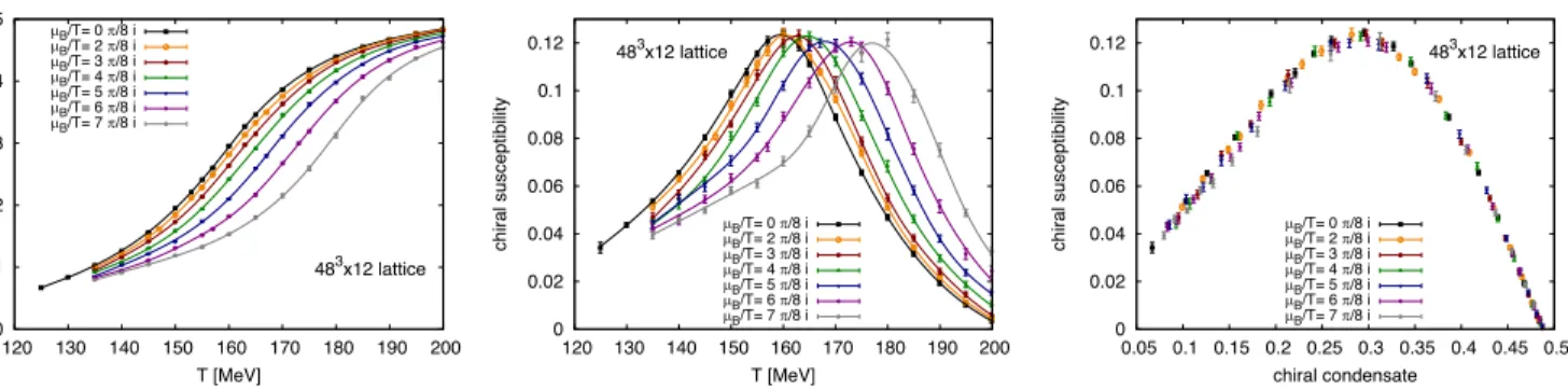
Our normalization choice in Eq. (2) was motivated by two observations, shown in Fig. 1 and explained below.
These observations (together with the improved statistics and the more accurate tuning ofμSðμBÞtonS¼0) allow a very precise determination ofTcas a function of imaginary chemical potential, which in turn allows a precise deter- mination of the parameters κ2 and κ4. We explored the chiral condensate and susceptibility in a broad range of imaginary baryochemical potential. In all panels of Fig.1, the black curves correspond to μB¼0. In the left and middle panel we show the chiral condensate and suscep- tibility as functions of the temperature. By construction, our renormalized condensate is zero atT ¼0 and positive at high temperature because of the explicit vacuum subtrac- tion and the overall negative sign in Eq.(2). In both panels, one can observe the shifting of the transition toward higher temperatures when an imaginary chemical potential is introduced. In the right panel we show the susceptibility as a function of the condensate. Here we converted the statistical error on the condensate into an additional error on the susceptibility by solving for hψψiðTÞ ¼¯ const and substituting the resulting T into χðTÞ (also taking the correlation of the statistical errors into account). Our first observation on the right panel of Fig.1is that the form of theχðhψψ¯ iÞcurve is simpler than that ofχðTÞ: a low-order (e.g., third or fourth) polynomial can fit the entire transition
0 0.1 0.2 0.3 0.4 0.5
120 130 140 150 160 170 180 190 200 483x12 lattice
chiral condensate
T [MeV]
PB/T= 0 S/8 i PB/T= 2 S/8 i PB/T= 3 S/8 i PB/T= 4 S/8 i PB/T= 5 S/8 i PB/T= 6 S/8 i PB/T= 7 S/8 i
0 0.02 0.04 0.06 0.08 0.1 0.12
120 130 140 150 160 170 180 190 200 483x12 lattice
chiral susceptibility
T [MeV]
PB/T= 0 S/8 i PB/T= 2 S/8 i PB/T= 3 S/8 i PB/T= 4 S/8 i PB/T= 5 S/8 i PB/T= 6 S/8 i PB/T= 7 S/8 i
0 0.02 0.04 0.06 0.08 0.1 0.12
0.05 0.1 0.15 0.2 0.25 0.3 0.35 0.4 0.45 0.5 483x12 lattice
chiral susceptibility
chiral condensate PB/T= 0 S/8 i PB/T= 2 S/8 i PB/T= 3 S/8 i PB/T= 4 S/8 i PB/T= 5 S/8 i PB/T= 6 S/8 i PB/T= 7 S/8 i
FIG. 1. Renormalized chiral condensate hψψi¯ (left) and chiral susceptibility χ (middle) as functions of the temperature for the intermediate lattice spacing in this study. The black curves correspond to vanishing baryon density, while results for various imaginary values of the chemical potential are shown in other colors. Finally, in the right panel we show the susceptibility as a function of the condensate. In this representation the chemical potential dependence is very weak.
range with an excellent fit quality. The second observation is that there is virtually no chemical potential dependence in theχðhψψiÞ¯ function. This way the susceptibility can be modeled as a low-order polynomial of two variables,hψψi¯ andμˆ ¼μB=T. Had we used a different normalization for the susceptibility, e.g.,χðTÞf4π=T4as we did in Ref.[5], the peak height would be strongly μB dependent and the collapse of the χðhψψiÞ¯ curves at different (imaginary) chemical potentials would not happen.
The transition line and its analytical continuation.—
Keeping the previous observations in mind, one can perform a precise determination of Tc, as defined by the peak of χ in Eq. (2), for various values of the imaginary chemical potential. Tcðμ2BÞ can then be fitted for the coefficients κ2 and κ4. This requires the following steps:
i) Determine the renormalized condensate hψψi¯ and susceptibility χ in a two-dimensional parameter scan in T and ImμB using lattice simulations. Use these to obtain the susceptibility as a function of the condensate. ii) Search for the peak ofχðhψψ¯ iÞthrough a low-order polynomial fit for eachNtand ImμBobtaininghψψi¯ cðNt;ImμBÞ. iii) Use an interpolation ofhψψiðTÞ¯ to convert thehψψ¯ ictoTc for each ImμB=T. iv) Perform a global fit ofTcðNt;ImμB=TcÞ to determine the coefficientsκ2 andκ4 for1=N2t ¼0. For this step we use various functions—all containing an independent κ6—with coefficients depending linearly on1=N2t.
There are ambiguities in steps i)–iv). We estimate their systematics by carrying out many versions of these steps.
For all these variations and the estimation of the errors, see the Supplemental Material [41]. We finally obtain
κ2¼0.01530.0018;
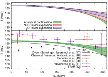
κ4¼0.000320.00067: ð3Þ We stress that the uncertainties on these two quantities are correlated. We put these results in the context of previous lattice studies in Fig.2. The extrapolated value ofTcðμBÞis shown in Fig.3(green band). Note that the errors onκ2and κ4 are dominated by the statistical errors, as shown in the detailed discussion of the systematic error estimate in the Supplemental Material [41].
Since Ref.[25]we have more than doubled the statistics and introduced a more precise analysis. The overall error on κ2has reduced slightly. The main result is the extraction of κ4. It appears to be a generic feature of deducing Taylor coefficients from polynomial fits: the increased precision on the input data leads to a sensitivity to a higher order coefficient first and only later to a reduction of the error of both coefficients. This feature is also clearly seen in the mock data analysis in the Supplemental Material[41].
In Fig. 3 we also show the comparison to the leading order Taylor expansion result (using onlyκ2) and the next to leading order result (usingκ2andκ4). The latter is very close to our full result (for μB<300MeV), while the
leading order result has a much smaller uncertainty.
Clearly, κ2 is precise enough. At intermediate μB, the bottleneck for the precision ofTcðμBÞis the error onκ4. We also fittedκ6, which turned out to be small enough to be irrelevant forμB <300MeV.
In Ref. [25] multiple Tc definitions were considered, leading to consistent values forκ2. However, none of those definitions can match the precision of theTc observable considered here, and precision was a prerequisite for the determination ofκ4.
Extrapolation of the transition width and strength.— A natural definition of the width of the susceptibility peak is given by its second derivative atTc as ðΔTÞ2¼
−χðTcÞ½ðd2=dT2Þχ−1T¼Tc. Unfortunately, evaluating this quantity is numerically difficult, so we introduce a simple width parameterσ as a proxy forΔT via
hψψiðT¯ cσ=2Þ ¼ hψψi¯ cΔhψψ¯ i=2; ð4Þ
withhψψi¯ c¼0.285andΔhψψi ¼¯ 0.14. The choice of the range in hψψi¯ is such that it is consistent with a linear behavior within our error bars, meaning that the ratio Δhψψi=σ¯ can be used as a proxy forðd=dTÞhψψij¯ T¼Tc as well. The exact range in hψψi¯ is chosen such that σ coincides with ΔT at zero and imaginary μB. A more detailed discussion of the width parameter can be found in the Supplemental Material[41].
We conclude that the half-width of the transition— shown in the upper panel of Fig.4—is consistent with a constant up toμB≈300MeV within the uncertainty from FIG. 2. Compilation ofκ4(left) andκ2(right) coefficients from recent lattice studies. We only include those papers where physical quark masses were used, a controlled continuum extrapolation was performed, and either strangeness neutrality or μs¼0 was considered. [Note that while μs¼0 means μS¼μB=3 for all values ofμB, strangeness neutrality impliesμS≈μB=4for small μB.] The colors encode the numerical approach. Blue points indicate simulations atμB¼0 only, where the μB dependence ofTc was extracted using a Taylor expansion. If a study used simulations with imaginary chemical potentials in addition, we plot the results with green points, instead. Top data points represent this work, the further references in order:[16,24,25,30].
the extrapolation (we note that 50% uncertainty is reached at μB≈280MeV).
Finally, as a proxy for the strength of the crossover, we study the value of the chiral susceptibility at the crossover temperature. We get this for each ImμB and Nt as a byproduct of steps i)–ii) of the analysis for κ2 and κ4. If one then performs a continuum extrapolation of the resulting values for fixed values of ImμB, one gets the lower panel of Fig. 4. Again, we see a very mild μˆ2B dependence, consistent with a constant.
Summary and discussion.—The main result of this work is a precise determination of the parametersκ2andκ4of the crossover line in finite density QCD. For the determination of the crossover line, we used the experimentally relevant μSðμBÞtuned to keepnS¼0. Based on the observation that the chiral susceptibility as a function of the condensate is a rather simple function, only weakly dependent on the imaginary chemical potential, we were able to obtain the transition temperature as a function of the imaginary chemical potential to very high accuracy. These pure lattice results can be used for further model building and are
summarized in the Supplemental Material [41]. The high precision data at imaginaryμBin turn allowed us to fit the μ2Bandμ4B Taylor coefficients of the crossover temperature κ2andκ4. In particular, while our determination ofκ4is still consistent with zero, the error is 6 times smaller than the one previously available in the literature and therefore represents the state of the art in the study of the phase diagram in theðT;μBÞplane with current lattice techniques.
As a byproduct, we also obtain the most precise value for the central temperature of the crossover atμB¼0so far, as well as the width of the transition:
TcðLT¼4;μB¼0Þ ¼158.00.6MeV
ΔTðLT¼4;μB¼0Þ ¼151MeV ð5Þ
We briefly discuss the meaning of these small errors in the Supplemental Material [41].
We also studied the strength of the phase transition as a function ofμBby extrapolating our proxy for the transition
0 10 20 30 40 50 60
0 50 100 150 200 250 300
V [MeV]
PB [MeV]
Proxy to the half width of the transition 0.215 < pbp < 0.355
0.00 0.02 0.04 0.06 0.08 0.10 0.12 0.14
0.1 0.15 0.2 0.25 0.3 0.35 0.4
F(pbp) 403x10 483x12 643x16
0.118 0.12 0.122 0.124 0.126 0.128 0.13 0.132 0.134 0.136
-8 -6 -4 -2 0 2 4
(PB/T)2 F(Tc)
FIG. 4. Top: Half-widthσ of the transition defined in Eq.(4) using the temperature difference of the contourshψψ¯ i ¼0.355 andhψψi ¼¯ 0.215. In the insert we show a plot of theχðhψψiÞ¯ peak, where the shaded region corresponds tohψψ¯ icΔhψψ¯ i=2. Both are extrapolated to realμB. Bottom: Result of aμBbyμB
analysis for the value of the chiral susceptibility at the crossover temperature after continuum extrapolation and including the systematic errors forLTc¼4. The green band shows a linear extrapolation inμˆ2B.
135 140 145 150 155 160
T [MeV]
Analytical continuation NLO Taylor-expansion LO Taylor-expansion
125 130 135 140 145 150 155 160 165 170
0 50 100 150 200 250 300
T [MeV]
µB [MeV]
Dyson-Schwinger: Isserstedt et al. [47]
Chemical freezeout: Andronic et al. [48]
Becattini et al. [49]
Alba et al. [50]
Vovchenko et al. [51]
STAR [52]
FIG. 3. Top: Transition line extrapolated from lattice simula- tions at imaginary chemical potential using an analytical con- tinuation with the ansatz used in step iv) of our analysis (green band) compared with an extrapolation using the formula in Eq.(1)up to the order ofκ4 (red band) or up toκ2(blue band).
The proximity of the full and NLO result suggests that the higher order corrections are small in the range ofμBconsidered here.
Note that considering only the error bar ofκ2underestimates the full error. The numerical values for the final analytical continu- ation, together with its error, are tabulated in the Supplemental Material[41]. Bottom: Crossover line from the lattice compared with a prediction from truncated Dyson–Schwinger equations [47]and some estimates of the chemical freeze-out parameters in heavy ion collisions [48–52]. Note that the width of the green band is not a representation of the width of the crossover region; it depicts the statistical and systematic errors achievable with the particular definition of the crossover temperatureTc adopted in this work. Note also that the definition of the crossover temperature adopted in Ref.[47] is different from the one used in this work.
width and the peak of the chiral susceptibility from imaginary chemical potentials. Even though one has to be careful with extrapolations, we see no sign of the transition getting stronger up toμB≈300MeV.
This project was funded by the DFG Grant No. SFB/
TR55. The project also received support from the BMBF Grant No. 05P18PXFCA. This work was also supported by the Hungarian National Research, Development, and Innovation Office, NKFIH Grant Nos. KKP126769 and K113034. A. P. is supported by the J. Bolyai Research Scholarship of the Hungarian Academy of Sciences and by the ÚNKP-19-4 New National Excellence Program of the Ministry for Innovation and Technology. This material is based upon work supported by the National Science Foundation under Grant No. PHY-1654219 and by the U.S. Department of Energy, Office of Science, Office of Nuclear Physics within the framework of the Beam Energy Scan Topical (BEST) Collaboration. The authors gratefully acknowledge the Gauss Centre for Supercomputing e.V. (www.gauss-centre.eu) for funding this project by providing computing time on the GCS Supercomputer JURECA/Booster at Jülich Supercomputing Centre (JSC), on HAZELHEN at HLRS, Stuttgart as well as on SUPERMUC-NG at LRZ, Munich. We acknowledge PRACE for awarding us access to Piz Daint hosted at CSCS, Switzerland. C. R. also acknowledges the support from the Center of Advanced Computing and Data Systems at the University of Houston.
[1] Y. Aoki, G. Endrodi, Z. Fodor, S. Katz, and K. Szabo, Nature (London)443, 675 (2006).
[2] T. Bhattacharya, M. I. Buchoff, N. H. Christ, H.-T. Ding, R. Gupta, C. Jung, F. Karsch, Z. Lin, R. Mawhinney, G. McGlynnet al.,Phys. Rev. Lett.113, 082001 (2014).
[3] Y. Aoki, Z. Fodor, S. Katz, and K. Szabo,Phys. Lett. B643, 46 (2006).
[4] Y. Aoki, S. Borsanyi, S. Durr, Z. Fodor, S. D. Katz, S. Krieg, and K. Szabo,J. High Energy Phys. 06 (2009) 088.
[5] S. Borsanyi, Z. Fodor, C. Hoelbling, S. D. Katz, S. Krieg, C.
Ratti, and K. K. Szabó (Wuppertal-Budapest Collaboration), J. High Energy Phys. 09 (2010) 073.
[6] A. Bazavov, T. Bhattacharya, M. Cheng, C. DeTar, H. Ding et al.,Phys. Rev. D85, 054503 (2012).
[7] C. Allton, S. Ejiri, S. Hands, O. Kaczmarek, F. Karsch, E.
Laermann, C. Schmidt, and L. Scorzato,Phys. Rev. D66, 074507 (2002).
[8] C. Allton, M. Doring, S. Ejiri, S. Hands, O. Kaczmarek, F.
Karsch, E. Laermann, and K. Redlich, Phys. Rev. D 71, 054508 (2005).
[9] R. V. Gavai and S. Gupta,Phys. Rev. D78, 114503 (2008).
[10] S. Basak et al. (MILC Collaboration), Proc. Sci., LATTICE2008 (2008) 171 [arXiv:0910.0276].
[11] S. Borsanyi, Z. Fodor, S. D. Katz, S. Krieg, C. Ratti, and K.
Szabó,J. High Energy Phys. 01 (2012) 138.
[12] S. Borsanyi, G. Endrodi, Z. Fodor, S. Katz, S. Krieg, C. Ratti, and K. K. Szabó, J. High Energy Phys. 08 (2012) 053.
[13] R. Bellwied, S. Borsanyi, Z. Fodor, S. D. Katz, A. Pasztor, C. Ratti, and K. K. Szabo, Phys. Rev. D 92, 114505 (2015).
[14] H. T. Ding, S. Mukherjee, H. Ohno, P. Petreczky, and H. P. Schadler,Phys. Rev. D92, 074043 (2015).
[15] A. Bazavovet al.,Phys. Rev. D95, 054504 (2017).
[16] A. Bazavovet al.,Phys. Lett. B795, 15 (2019).
[17] A. Bazavovet al.,Phys. Rev. D101, 074502 (2020).
[18] P. de Forcrand and O. Philipsen,Nucl. Phys. B642, 290 (2002).
[19] M. D’Elia and M.-P. Lombardo,Phys. Rev. D 67, 014505 (2003).
[20] M. D’Elia and F. Sanfilippo, Phys. Rev. D 80, 014502 (2009).
[21] P. Cea, L. Cosmai, and A. Papa,Phys. Rev. D89, 074512 (2014).
[22] C. Bonati, P. de Forcrand, M. D’Elia, O. Philipsen, and F. Sanfilippo,Phys. Rev. D90, 074030 (2014).
[23] P. Cea, L. Cosmai, and A. Papa,Phys. Rev. D93, 014507 (2016).
[24] C. Bonati, M. D’Elia, M. Mariti, M. Mesiti, F. Negro, and F. Sanfilippo,Phys. Rev. D92, 054503 (2015).
[25] R. Bellwied, S. Borsanyi, Z. Fodor, J. Günther, S. D. Katz, C. Ratti, and K. K. Szabo,Phys. Lett. B751, 559 (2015).
[26] M. D’Elia, G. Gagliardi, and F. Sanfilippo,Phys. Rev. D95, 094503 (2017).
[27] J. Gunther, R. Bellwied, S. Borsanyi, Z. Fodor, S. D. Katz, A. Pasztor, and C. Ratti,EPJ Web Conf.137, 07008 (2017);
Nucl. Phys.A967, 720 (2017).
[28] P. Albaet al.,Phys. Rev. D96, 034517 (2017).
[29] V. Vovchenko, A. Pasztor, Z. Fodor, S. D. Katz, and H. Stoecker,Phys. Lett. B775, 71 (2017).
[30] C. Bonati, M. D’Elia, F. Negro, F. Sanfilippo, and K. Zambello, Phys. Rev. D98, 054510 (2018).
[31] S. Borsanyi, Z. Fodor, J. N. Guenther, S. K. Katz, K. K.
Szabo, A. Pasztor, I. Portillo, and C. Ratti,J. High Energy Phys. 10 (2018) 205.
[32] Z. Fodor and S. Katz,J. High Energy Phys. 03 (2002) 014.
[33] Z. Fodor and S. Katz,J. High Energy Phys. 04 (2004) 050.
[34] Z. Fodor, M. Giordano, J. N. Günther, K. Kapás, S. D. Katz, A. Pásztor, I. Portillo, C. Ratti, D. Sexty, and K. K. Szabó, Nucl. Phys.A982, 843 (2019).
[35] M. Giordano and A. Pasztor, Phys. Rev. D 99, 114510 (2019).
[36] S. Mukherjee and V. Skokov,arXiv:1909.04639.
[37] M. Giordano, K. Kapas, S. D. Katz, D. Nogradi, and A. Pasztor,Phys. Rev. D101, 074511 (2020).
[38] O. Kaczmarek, F. Karsch, E. Laermann, C. Miao, S. Mukherjee, P. Petreczky, C. Schmidt, W. Soeldner, and W. Unger,Phys. Rev. D83, 014504 (2011).
[39] G. Endrodi, Z. Fodor, S. Katz, and K. Szabo,J. High Energy Phys. 04 (2011) 001.
[40] K. Zarembo,Pis’ma Zh. Eksp. Teor. Fiz.110, 147 (2019) [JETP Lett.110, 155 (2019)].
[41] See Supplemental Material at http://link.aps.org/
supplemental/10.1103/PhysRevLett.125.052001 for the technical details of this study, which includes Refs. [42–46].
[42] M. Tanabashiet al.(Particle Data Group),Phys. Rev. D98, 030001 (2018).
[43] S. Borsanyi, S. Durr, Z. Fodor, C. Hoelbling, S. D. Katz et al.,J. High Energy Phys. 09 (2012) 010.
[44] S. Borsanyiet al.,Nature (London)539, 69 (2016).
[45] R. Bellwied, S. Borsanyi, Z. Fodor, J. N. Guenther, J. Noronha-Hostler, P. Parotto, A. Pasztor, C. Ratti, and J. M. Stafford,Phys. Rev. D101, 034506 (2020).
[46] C. Bonati, M. D’Elia, M. Mariti, M. Mesiti, F. Negro, and F. Sanfilippo,Phys. Rev. D90, 114025 (2014).
[47] P. Isserstedt, M. Buballa, C. S. Fischer, and P. J. Gunkel, Phys. Rev. D100, 074011 (2019).
[48] A. Andronic, P. Braun-Munzinger, and J. Stachel, Nucl.
Phys.A772, 167 (2006).
[49] F. Becattini, M. Bleicher, T. Kollegger, T. Schuster, J.
Steinheimer, and R. Stock, Phys. Rev. Lett. 111, 082302 (2013).
[50] P. Alba, W. Alberico, R. Bellwied, M. Bluhm, V. Mantovani Sarti, M. Nahrgang, and C. Ratti, Phys. Lett. B 738, 305 (2014).
[51] V. Vovchenko, V. V. Begun, and M. I. Gorenstein, Phys.
Rev. C93, 064906 (2016).
[52] L. Adamczyket al.(STAR Collaboration),Phys. Rev. C96, 044904 (2017).