Spot Price Models for Natural Gas

(1)

Spot Price Models for Natural Gas

-

Robustness of the Convenience Yield Approach

Thomas Volmer

March 31, 2011

(2)

Dissertation

zur Erlangung des Doktorgrades an der

Fakultät Sozial- und Wirtschaftswissenschaften der Otto-Friedrich-Universität Bamberg

Vorgelegt von:

THOMAS VOLMER

Erstprüfer: Prof. Dr. Matthias Muck, Otto-Friedrich-Universität Bamberg

Zweitprüferin: Prof. Dr. Susanne Rässler, Otto-Friedrich-Universität Bamberg

Tag der mündlichen Prüfung: 21. Dezember 2011

(3)

Acknowledgements

I am particularly grateful to Matthias Muck, my supervisor, for his in- valuable support during my dissertation project. Without our numerous discussions and his advice I would not have been able to compose this work. I would also like to thank Susanne Rässler who provided me with helpful statistical guidance several times. She also kindly agreed to be part of my dissertation committee.

Furthermore, my work has strongly pro…ted from fruitful discussions at the University of Bamberg with my colleagues from the Chair of Financial Control. I am especially grateful to Jan Marckho¤ and Sebastian Paik for their enriching feedback and suggestions in many di¢ cult situations. I would also like to thank the team of the Chair for the enjoyable working atmosphere during my time in Bamberg.

Moreover, many thanks go to Bagher Modjtahedi and Richard Quandt from the US as well as Scott Chaput and Martin Hill from New Zealand and Australia, respectively, for their helpful support and comments regard- ing my …rst paper. Additionally, I thank participants at the 13th Confer- ence of the Swiss Society for Financial Markets Research (SGF) in Zurich and at the Conference on Energy Finance at the University of Agder, Kristiansand, Norway. Many thanks also go to APX-ENDEX, the British Atmospheric Data Center (BADC), the Intercontinental Exchange (ICE), the International Energy Agency (IEA) and National Grid UK for kindly providing the data used in my dissertation. I would like to highlight the personal support of Vlad Kaltenieks from APX-ENDEX and Rajesh Kuka- dia from National Grid who dealt with several of my individual queries.

Finally, I am greatly indebted to Kathrin, my family and friends for

their emotional support and encouragement as well as their enduring belief

in my dissertation project.

(4)

iv

To my family

(5)

List of Tables

5.1 Estimation results of basic convenience yield model . . . . . 69 5.2 Estimation results of squared stock model . . . . 80 5.3 Estimation results of regime-switching model . . . . 82 5.4 Estimation results when controlling for crude oil price changes 86 5.5 Estimation results when controlling for the conv. yield of

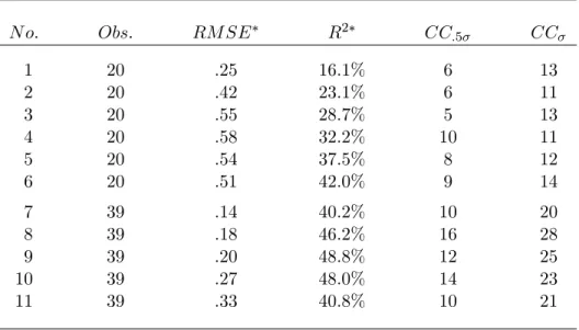
crude oil . . . . 88 5.6 Results of in-sample robustness test for basic model . . . . 91 5.7 Result of in-sample robustness test for squared stock model 92 5.8 Diagnostics for out-of-sample forecast of squared stock model 95 5.9 Regression results for squared stock model using deseas.

daily data . . . 100 6.2 Summary statistics for convenience yields . . . 122 6.3 Regression results for convenience yield model in US . . . . 123 6.4 Simulation results of the estimation routine for the reduced-

form model . . . 134

viii

(9)

LIST OF TABLES ix 6.5 Estimation results of the SCY-model for the UK using the

Kalman …lter . . . 136 6.6 Goodness-of-…t statistics for the UK market . . . 141 6.7 Estimation results of the SCY-model for the US using the

Kalman …lter . . . 143 6.8 Goodness-of-…t statistics for the US market . . . 146 6.9 Estimation results with changing sets of maturities . . . 147 6.10 Bayesian estimation results for the extended model (US data)158 6.11 Bayesian estimation results for short and long maturities

(US data) . . . 161

6.12 Simulation results using implied parameter estimates . . . . 168

6.13 Estimation results using implied parameter estimates . . . . 171

(10)

List of Figures

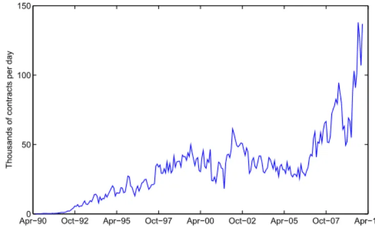
2.1 Historical volumes of gas futures traded at the NYMEX . . 9

2.2 Price di¤erential along the interconnector (Bacton - Zee- brugge) . . . . 13

2.3 Daily prices of the 3-month ahead future in UK . . . . 13

3.1 Binomial tree scheme . . . . 31

5.1 Historical time series of convenience yield in UK . . . . 66

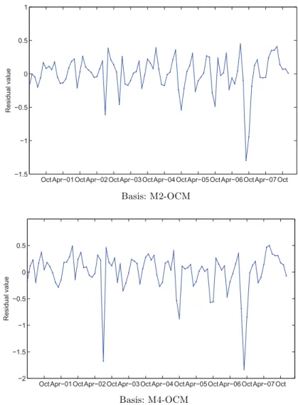
5.2 Plots of residuals from basic model against stocks . . . . 72

5.3 Plots of residuals from basic model against time . . . . 73

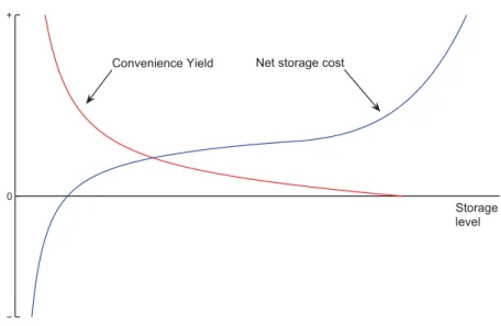
5.4 Net storage cost as a function of storage levels (Brennan, 1958) . . . . 75

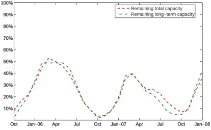
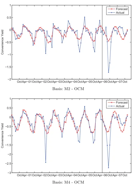
5.5 Residuals of basic model vs. remaining storage space (UK) . 84 5.6 Selected plots of convenience yield forecasts out of the sample 96 6.1 Spot price drift: Standard vs. extended model . . . 113

x

(11)

LIST OF FIGURES xi 6.2 Historical weekly settlement prices of NYMEX front month

future . . . 119

6.3 Comparison of seasonal …tting for US and UK futures . . . 126

6.4 Histograms of US futures price changes . . . 127

6.5 Filtered vs. actual/measured values of state variables in UK 139

6.6 Filtered versus actual values of futures in UK . . . 140

6.7 Measurement errors of the standard SCY model (US) . . . 151

6.8 Prior and post. distribution of parameters with US data (1) 156

6.9 Prior and post. distribution of parameters with US data (2) 157

6.10 Prior and post. distribution of parameters with US data (3) 160

6.11 Prior and post. distribution of parameters with US data (4) 162

6.12 Prior and post. distribution of parameters with US data (5) 163

6.13 Prior and post. distribution of parameters with US data (6) 164

6.14 Analysis of estimation bias for 2 using implied estimates . 167

6.15 Implied against …ltered state variables (US) . . . 170

(12)

List of Abbreviations

APX Amsterdam Power Exchange BADC British Atmospheric Data Centre bcm billion cubic meters

BOM balance of the month CIR Cox, Ingersoll and Ross

ch. chapter

c.p. ceteris paribus

EEX European Energy Exchange

EIA Energy Information Administration

eq. equation

FERC Federal Energy Regulatory Commission FGLS feasible generalized least squares

fn. footnote

xii

(13)

xiii GBM geometric Brownian motion

ICE Intercontinental Exchange IEA International Energy Agency MAE mean absolute error

mcm million cubic meters

ME mean error

ML maximum likelihood

MMA money market account

MWh megawatt hours

mmBtu million British thermal units NBP National Balancing Point

OCM On-the-Day Commodity Market (UK) OTC over the counter

p. page

PDE partial di¤erential equation RMSE root mean squared error SCY stochastic convenience yield

vs. versus

SDE stochastic di¤erential equation

sec. section

w.r.t. with respect to

(14)

List of Symbols

Latin letters

A(T ) deterministic, parametric function of maturity T of Schwartz (1997)

B value of money market account

C amount of storage cost or amount of consumption good available (sec. 4.4)

D basis di¤erential (ch. 2) or D-value of Goldfeld and Quandt (1972)

F forward or futures price

H covariance matrix of measurement errors (Kalman …l- ter)

I inventory level

J value function

K option strike price

L value of the likelihood function

xiv

(15)

xv Mi month future with maturity in the ith-next month N length of time series

O stock of explored oil

P value of replicating portfolio (ch. 3, ch. 6) or inverse demand function (ch. 4) or marginal amount of storage risk premium (ch. 5)

P empirical probability measure

Q marginal amount of convenience yield (ch. 5) or state noise covariance matrix (Kalman …lter, ch. 6)

Q risk-neutral probability measure

R marginal amount of interest (ch. 5) or error sensitivity matrix (Kalman …lter, ch. 6)

R ² coe¢ cient of determination

S spot price

T transition matrix (Kalman …lter) U jump size or utility function (sec. 4.4)

X "amount on hand" or exploration quantity (sec. 4.4) or log-spot price

Z exogenous production quantity or design matrix (Kalman …lter)

c storage cost rate (% of spot price) or vector of constants

(Kalman …lter)

(16)

xvi LIST OF SYMBOLS d di¤erential operator or vector of constants (Kalman …l-

ter)

dN increment of Poisson process dW increment of Wiener process

f function

i index (integer)

k risky rate of return

m net cost of storage (ch. 5) or state size (Kalman …lter) n number of elements/observations in subsample or cross-

section

r (riskless) interest rate t time index or current period

u marginal revenue of storage (sec. 5.1) or autocorrelated residual

v portfolio weight

v (risk-neutral) spot price drift

x dependent variable

y independent variable

Greek letters

di¤erence operator

parameter set

(17)

xvii mean-reversion level (stochast. processes) or state vec- tor (Kalman …lter)

regression coe¢ cient rate of storage depreciation

convenience yield rate (% of spot price) residual or measurement noise (Kalman …lter) residual or state noise (Kalman …lter)

mean-reversion level (ch. 4) or deseas. convenience yield rate (ch. 6)

mean-reversion coe¢ cient market risk premium

P Poisson intensity of jumps deterministic drift rate

long-term risk factor of Schwartz and Smith (2000) or measurement error standard deviation (ch. 6)

coe¢ cient of correlation or rate of storage risk premium (ch. 5)

standard deviation

short-term risk factor of Schwartz and Smith (2000) or portfolio weight (ch. 6)

coe¢ cient of autocorrelation

portfolio weight

(18)

xviii LIST OF SYMBOLS

Decorations and superscripts

^ estimate of theoretical counterpart

e alteration of a quantity previously de…ned

risk-neutral parameter or FGLS-transormed coe¢ cients (ch. 5)

e estimate of the theoretical counterpart

s deseasonalized variable

(19)

Chapter 1

Introduction

In recent years exchange traded natural gas contracts have gained great importance. This especially applies to continental Europe where increased liberalization and transparency are now on the agenda. One fact underpin- ning the rising interest in standardized contracts is the recent start of gas trading at several energy exchanges in this region. In July 2007 the Ger- man EEX (European Energy Exchange) launched its gas trading platform.

In May and November 2008, respectively, the Scandinavian Nord Pool and the French Powernext followed suit. Finally, in December 2009 and 2010, respectively, Central European Gas Hub launched the Gas Spot and Gas Futures segments at Wiener Börse. Further support can be found by look- ing at the exchange traded volumes at the more established continental hubs: APX-ENDEX recently reported a year-on-year volume increase of 130% in gas trading at the Dutch TTF to 210 TWh in 2010 and a 22%

increase for the Belgian hub Zeebrugge to 203 MWh in 2010. ¹

Along with the importance of exchange traded gas grows the necessity to …nd accurate pricing models for the di¤erent contract types and this

1

Cf. APX-ENDEX (2011), p. 20.

1

(20)

2 INTRODUCTION regularly requires a future spot price. That said, one notable di¤erence between commodities and stocks or bonds is that the current spot price is not directly observable in the market. During the last few decades a number of general commodity pricing models have been developed and tested. However, the application to natural gas pricing was predominantly tested using reduced-form models such as the well-known two-factor mod- els by Gibson and Schwartz (1990), Schwartz (1997) and Schwartz and Smith (2000). As opposed to structural models, these models build on an exogenously speci…ed stochastic process rather than supply and demand conditions founded in microeconomic theory. They are mostly uncomplex and also capture typical phenomena of the forward curve (e.g. the Samuel- son e¤ect ² ), but they do not o¤er fundamental economic explanations for the predicted prices.

The lack of insight into the real price drivers is a downside of pure reduced-form models because the risk of misspeci…cation is high and the out-of-sample performance can be poor. With respect to the Schwartz and Smith model, Carlson et al. (2007) show that given frictional production adjustments in the oil and gas market the model will systematically over- estimate the prices for oil and gas options. Similarly, Ribeiro and Hodges (2004) …nd that “. . . the use of current reduced-form models in the litera- ture to price energy contingent claims has not been e¤ective. In particular, the convenience yield process seems to be misspeci…ed since its speci…ca- tion ignores some crucial properties of commodity price behavior such as the dependency of prices’variability on inventory levels” (p. 3).

Beyond the general criticism of reduced-form commodity price models, the latter statement points at di¢ culties caused by a speci…c price com-

2

The Samuelson e¤ ect describes the fact that the volatility of forward prices increases

with decreasing time to maturity and is due to the mean reverting property of many

commodity spot prices.

(21)

INTRODUCTION 3 ponent: the convenience yield. The concept of convenience yield originates from Kaldor (1939), the groundwork of the ‘ theory of storage’ . Kaldor states that goods in stock which are not yet sold forward have an unob- servable ‡exibility yield because market participants owning these goods have the ‘convenience’ to make use of them whenever wanted. ³ For this reason, according to Kaldor, the observable cost of carry of a stored com- modity, that is foregone interest and the outlay on physical storage, must be reduced by this availability premium. Brennan (1958) and Telser (1958) have further established that this premium varies with the level of storage in the economy. The concept of convenience yield is explained in detail in chapter 5.

The idea that such an availability premium impacts the spot price has also been implemented in a number of reduced-form commodity models.

However, Schwartz and Smith (2000) abandon the concept of convenience yield in their generalized two-factor model and simply use a ‘long-term’

and a ‘short-term’price component, one reason being that “[...] many …nd the notion of convenience yield elusive [. . . ]”(p. 894). Given that the basic theory of the convenience yield is widely accepted, it seems questionable to neglect this variable in up-to-date pricing models since it contains funda- mental economic information. Apparently, economists are simply lacking considerable knowledge about the dynamic behavior of the convenience yield in speci…c markets. Possession of such information would enable the economist to generate fundamental forecasts and to integrate them into a reduced-form model as an exogenous component. This could help to reduce the uncertainty in spot price forecasting signi…cantly. At the same time, it

3

This ‡exibility is of value since contrary to the owner of shares or bonds a commodity

owner can put this good to additional use, for exapmle in industrial production. If there

is uncertainty about the time when the input factor is needed, the producing company

is more ‡exible by holding the commodity upfront than by entering a long postion in a

forward contract with a …xed delivery date.

(22)

4 INTRODUCTION might constitute a viable compromise between the complexity of structural models and the danger of misspeci…cation in reduced-form approaches.

The following study is based on this motivation and the aforementioned increase in demand for exchange-traded risk management instruments in the natural gas market, particularly in continental Europe. Therefore, in the …rst half of the main part, we present an econometric analysis of the drivers of convenience yield for natural gas. As a …rst contribution, it is shown that, in addition to national gas storage levels, air temperature is a highly relevant and robust determinant of the convenience yield. Moreover, a regime-switching model, although not optimal for predictions, makes explicit that basis variability in gas markets rises with inventories as long as the average observed inventory is su¢ ciently high. This contrasts …ndings of Fama and French (1987) for non-energy commodities, and it will be argued that the opposing behavior is due to the capacity constraints of underground gas storage. Kogan et al. (2009) document similar …ndings for crude oil futures prices. In addition, to the best of our knowledge, we are the

…rst to investigate the robustness of a convenience yield model for pricing applications. A forecasting exercise, which identi…es the squared storage model as the most appropriate speci…cation, is presented afterwards. It is shown that the model keeps its explanatory power when the measurement interval is varied.

In the second half of the main part, we use the convenience yield model

to develop a new model for the gas spot price based on the stochastic con-

venience yield model (SCY model ) of Schwartz (1997). First, to estimate

this extended model, futures prices are netted of those deviations from

the equilibrium price which are explained by the fundamental variables

above. Next, the model is estimated with the "netted" prices. Then, the

prediction results are compared to those generated with the unmodi…ed

futures price data. It is shown that the extended model improves the out-

of-sample forecast as the forecast horizon increases. At the same time, the

(23)

INTRODUCTION 5 in-sample and the cross-sectional …t are at least as good as for the bench- mark. Nevertheless, conceptual and also numerical reasons lead to the fact that, irrespective of the model version, parameter stability along the cross- section of futures contracts leaves room for further amendments. For this reason, the study concludes with an in-depth analysis of alternative es- timation methods. Yet, we …nd that these alternatives are not favorable to the standard method, i.e. a maximum likelihood estimation with the Kalman …lter. Since the gas market is regionally fragmented ⁴ and for some additional reasons ⁵ , the …rst part of the study is conducted on the liberal- ized UK gas market. Additionally, the scope is then extended to cover the US market.

The structure of the thesis is as follows: Firstly, in chapter 2, we explain why increased demand for …nancial risk management products has been arising in the gas market for a number of years. It is argued that this makes it worthwhile and necessary to …nd accurate pricing models for these emerging …nancial instruments. Next, the study discusses why gas needs to be studied separately from other commodities that have already received more research attention. It is also addressed why the UK and the US are suitable markets to study. The chapter closes with an overview of the most important risk management products for natural gas and leads over to the reason for the particular importance of the future spot price (and hence spot price models) in risk management. Chapter 3 elaborates on the two most important analytical methods for derivative pricing in

…nancial theory and gives a brief overview of more advanced techniques.

Chapter 4 presents and classi…es existing models of spot (and forward)

4

Geman (2006), for instance, distinguishes between the 3 regional markets: America, Europe and Asia.

5

One practical advantage over the even more developed US market is that climate con-

ditions are su¢ ciently uniform within this market which facilitates our econometric

analysis. Further details are provided during the course of the study.

(24)

6 INTRODUCTION

prices for energy commodities. The models are brie‡y evaluated according

to a set of de…ned requirements. In addition, we explain why we choose

the SCY model as the starting point for our model extension. In the main

part, the determinants of convenience yield (chapter 5) and a hybrid spot

price model with fundamental convenience yield forecasts (chapter 6) are

investigated. The last chapter concludes.

(25)

Chapter 2

The natural gas market

In this chapter we illustrate, …rst of all, why …nancial risk management in natural gas has become an interesting and relevant …eld of research.

Next, we explain why natural gas has to be modelled individually, i.e.

why the existing research on the pricing of energy derivatives is not su¢ - cient to build a reliable gas price model. Afterwards, we show that the gas markets of the UK and the US are most suitable for an empirical study.

More precisely, we illustrate the di¤erence of trading in liberalized vs. non- liberalized markets and classify both the British and the American market as rather liberalized. The last section of this chapter gives an overview about the derivatives which are actually traded in the natural gas mar- ket. It will be concluded that their payo¤s regularly depend (directly or indirectly) on the future spot price. This is the ultimate reason for our objective to search for the most adequate spot price model.

7

(26)

8 CHAPTER 2. THE NATURAL GAS MARKET

2.1 Liberalization of natural gas markets

Open access to the distribution and sales segment of the US gas market was e¤ectuated by the FERC orders 436 and 500 in 1985. They allowed end customers to buy directly from producers by reserving capacity on in- terstate pipelines. In the aftermath, di¤erent tari¤ structures and service levels evolved, such as …rm and interruptible service of di¤erent degrees. In 1992, FERC …nal order 636 enforced the unbundling of pipeline services.

It was now permitted to transfer unused …rm transportation capacity to a third party. These orders together are responsible for the strong increase in business activity during the 1990s (cf. Figure 2.1). ¹ In the years after the collapse of Enron in late 2001, US gas trading volumes entered into a phase of stagnation. However, since 2006, the massive in‡ux of capital from

…nancial investors, notably hedge funds, has led to a tripling of turnover and a corresponding push in market liquidity until today. In fact, this re- cent development in the world’s biggest natural gas market best illustrates the rising importance of the commodity.

In Europe, the UK started deregulation in the mid-eighties. The Nat- ural Gas Act of 1986 lead to the privatization of the formerly state-owned British Gas. The tari¤ market, the market segment for small-scale con- sumers, became regulated through a price cap while the contract market for large-scale clients remained, in fact, a monopoly until the mid-nineties.

In 1995, the reform of the Natural Gas Act opened the whole residential market for competition until 1998. The threshold consumption quantity for clients’access to the contract market was gradually lowered until 1997, squeezing out the monopolistic tari¤ segment. The milestone of the liberal- ization process was the ultimate unwinding of transportation (BG Transco)

1

Cf. Sturm (1997), ch. 1.

(27)

2.1. LIBERALIZATION OF NATURAL GAS MARKETS 9

Apr−900 Oct−92 Apr−95 Oct−97 Apr−00 Oct−02 Apr−05 Oct−07 Apr−10 50

100 150

Thousands of contracts per day

Figure 2.1: Daily volumes of natural gas month futures traded at the NYMEX (monthly averages, front month contract).

and storage from the exploration business (Centrica) in 1997. ²

Deregulation in Continental Europe has been lagging behind. In 1998 the European Parliament and Council formulated the Directive on the In- ternal Market in Natural Gas I (1998/30/EC), but the speed with which member states promoted the national market opening varied considerably.

Italy, the Netherlands and Spain, for instance, had already shown pro- gressive developments until the publication of the second benchmarking report in October 2002, whereas Germany had not implemented the above Directive even by mid-year 2003. The second directive (2003/55/EC) and Regulation 1775/2003 set more ambitious targets in many respects. Free choice of supplier had to be established for all B2B customers by mid-year 2004 and for residential customers by mid-year 2007 in all member states.

2

Cf. Price (1997).

(28)

10 CHAPTER 2. THE NATURAL GAS MARKET Unused capacity had to be o¤ered to third parties. Integrated gas under- takings had to legally and organizationally separate their transportation and distribution from their exploration and production businesses. How- ever, legal unbundling of the distribution system has still been subject to a postponement option. For this reason, the liberalization process has continued to progress with di¤erent speed in the member states. ³

On a macroeconomic level, market structures in Continental Europe remain ine¢ cient to date. One reason is that roughly 90% of volumes contracted in these markets are long-term take-or-pay contracts. Hence, short-term volume and price risk might not always be optimally distributed between supply and demand at present. Yet, it is envisioned by a number of experts that long-term contracts will loose some importance and that a greater fraction of gas will soon be traded on exchanges. For instance, Neumann and von Hirschhausen (2004) point out that “[. . . ] the empirical evidence from the US and the UK suggests an inverse relationship between gas sector liberalization and contract length, although long-term contracts do not entirely disappear with market liberalization” (p. 177). The demand for risk management in Continental Europe will hence continue to rise and e¤orts to deepen the understanding of the underlying price risk may constitute an important research contribution.

2.2 Properties of gas as a commodity

According to the IEA, natural gas accounted for 21% of global primary energy demand in 2008, and its share will increase to 25% by 2035, while oil is projected to drop from 33% to 27% in the same period. The most important rise in gas consumption in absolute terms will come from elec-

3

Cf. Haase (2008).

(29)

2.2. PROPERTIES OF GAS AS A COMMODITY 11 tricity generation, whose share will increase from 21% of total gas demand in 2008 to 24% in 2035. ⁴ The main drivers of the projected growth are global climate concerns and the corresponding national commitments to reduce greenhouse gas emissions. Since gas-…red power plants operate with much lower CO ₂ emissions than coal plants, some important CO ₂ produc- ers like China plan to replace an important part of their current generation capacity.

Natural gas is a very speci…c commodity. As opposed to many other energy carriers, pipelines are the predominant medium for transportation.

Long-distance transportation necessitates repressurizing the gas after a certain distance which is an energy-intensive process. This adds to the maintenance of metering stations and pipelines such that the total trans- portation cost per unit of calori…c value is …ve times higher than for oil.

Since the pipeline system has a limited reach and supply and demand cen- ters are not evenly distributed over the world, regional markets instead of a single world market have developed. This is contrary to the oil market, in which transportation by tankers is an economical alternative to pipelines and a single contract per sort is traded worldwide. ⁵ . Geman (2006) dis- tinguishes three di¤erent demand regions for gas: North America, Europe and Asia. Even within one of these markets, prices can di¤er substantially depending on the capacity to transport gas to the location of maximum scarcity. This can lead to persistent demand-supply imbalances and hence to intra-regional price di¤erences.

The gas price re‡ects these facts in di¤erent forms. If short-term im- balances in the intra-regional ‡ows of gas occur, price jumps or spikes are a common consequence. They can especially be observed on an intraday basis. This type of imbalance is mainly due to the prominent role of gas in

4

Cf. IEA (2011), GAS scenario.

5

Cf. Geman (2006), p. 236, Shively and Ferrare (2007), ch. 4.

(30)

12 CHAPTER 2. THE NATURAL GAS MARKET power generation, but can also be caused by disruptions in production or pipeline operations. ⁶ Medium-term intra-regional price imbalances last for a day or longer and can be due to insu¢ cient pipeline capacity between di¤erent market areas in the considered region. A prominent example is the price di¤erence between gas at the National Balancing Point (NBP), the main hub in UK, and the hub Zeebrugge (Belgium). Such a situation can be due to overbooking of the interconnector pipeline which links the two regions. Maintenance operations and time lags in the process of re- versing the ‡ow direction do also play an important role. Figure 2.2 shows the daily price di¤erential between the two market areas in percent of the mean of the two prices. As can be seen, the di¤erential is substantial overall. Moreover, the daily di¤erentials are obviously not independently and symmetrically distributed, but skewed with clustered volatility. These ine¢ ciencies are due to the grid-boundedness of the commodity.

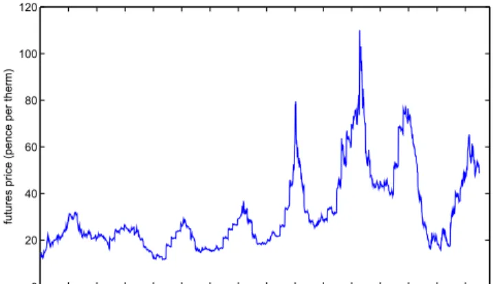
Apart from intra-regional disequilibria, there are repeating patterns of price changes caused by annual seasonality in demand. In the winter, space heating demand drives up prices. In the US, prices also rise in the summer due to the prominent role of air conditioning which increases gas demand from power stations. Figure 2.3 shows the daily quotes of the UK 3-month ahead (M3) gas future traded on the Intercontinental Exchange (ICE). One can observe an annual price peak at the beginning of the winter season when the deliveries for the coldest months (January and February) are traded.

Furthermore, storage does not even out the seasonality and short-term

‡uctuations signi…cantly. In fact, storage technologies in the industry are very speci…c because gas is stored underground. Since this is very costly, it takes a considerable intertemporal price di¤erence to have agents use

6

The works of Douglas and Popova (2008) and Routledge et al. (2001) look at the price

relationship between gas and power in detail.

(31)

2.2. PROPERTIES OF GAS AS A COMMODITY 13

Aug−07 Dec−07 May−08 Sep−08 Feb−09 Jul−09 Nov−09 Apr−10 Aug−10

−40%

−20%

0%

20%

40%

60%

80%

100%

Price differential Zeebrugge (B) − Bacton (UK)

Figure 2.2: Daily price di¤erential of day-ahead gas along the interconnec- tor (Bacton - Zeebrugge) in % of the mean price.

OctApr−01OctApr−02OctApr−03OctApr−04OctApr−05OctApr−06OctApr−07Oct 0

20 40 60 80 100 120

futures price (pence per therm)

Figure 2.3: Daily prices of the 3-month ahead future in UK.

(32)

14 CHAPTER 2. THE NATURAL GAS MARKET storage. In addition, the exploration of new storage space can take a long time, and the required amount of capital can be substantial. The geological formations which are commonly exploited for gas storage are depleted gas and oil …elds, salt caverns and aquifers. The …rst type of formation is nor- mally the largest and the least costly to develop. However, the storage cycle time is the lowest such that these facilities can only o¤er seasonal storage.

Aquifers have higher deliverability rates and gas can be cycled more than once per season. However, they have high base gas requirements ⁷ and bear a high degree of geological risk. Salt caverns, in turn, have very low base gas requirements, an even higher deliverability and almost no geological risk. In turn, the exploration cost is extremely high. ⁸ Brie‡y, the high investment and operating expenses of gas storage can lead to structural shortages of available storage space in the market. If the growth of a mar- ket’s storage capacity does not keep pace with the growth of demand, price volatility will increase. The same will happen if supply uncertainty rises for which the UK market is a prominent example. ⁹

To summarize, this section has shown that gas is an economically rele- vant commodity and that some of its fundamental properties suggest an in- dividual modelling. The most important properties in comparison to other energy carriers are the grid-boundedness, the pronounced daily and sea- sonal ‡uctuations of demand and prices as well as the costly storage tech- nology. Next, it is explained how trading in gas markets works in order to justify the choice of markets for the empirical analysis.

7

The gas which remains in a storage facility to keep pressure at a su¢ cient level (also called cushion gas).

8

Cf. Dietert and Pursell (2000).

9

See section 5.3, p. 64 for details on the case of the UK.

(33)

2.3. TRADING IN LIBERALIZED VS. REGULATED MARKETS 15

2.3 Trading in liberalized vs. regulated markets

A “commodity” in the sense of …nancial theory is not only de…ned by the nature of the good and its time of delivery, but also by its quality and delivery location. The last mentioned aspect is especially relevant for grid- bound commodities such as natural gas. This means that, for instance, natural gas somewhere in California is a di¤erent commodity than natural gas in New York City. Regarding quality, a given volume of natural gas can have a varying chemical composition. In Western Europe, there are currently two di¤erent networks for gas with high calori…c value (H-gas) and low calori…c value (L-gas). In the US, there is no such distinction. In addition to these properties, natural gas is sold for delivery over a period of time rather than at a point in time. This is due to the fact that the possibility of storing gas at the location of demand is usually very limited.

These features are relevant for any type of supply contract presented in the following.

Given the importance of the delivery location, it becomes immediately clear that standardized and e¢ cient trading operations are only possible if the commodity is priced with respect to a single reference point. In the natural gas market, the so-called hubs, i.e. interconnects of a number of long-distance pipelines, serve as such point. The reason for this is that, in any case, most of the gas traded in the respective region or market area has to pass the hub in order to be shipped from the supplier to the customer. Hubs do not necessarily exist physically, but can be virtual as well. A virtual hub is an area rather than a speci…c point in the network.

Henry Hub in Louisiana is an example of a physical gas hub whereas the NBP in the UK is a virtual hub.

The mentioned hubs are examples from liberalized markets in which

network access to deliver gas to the hub is non-discriminatory and non-

(34)

16 CHAPTER 2. THE NATURAL GAS MARKET frictional. Non-discriminatory means that every market agent who wants to o¤er gas is allowed and able to book pipeline capacity from any entry point of the pipeline system to the hub. Non-frictional means that the cost of shipping is not excessive. The following example illustrates this criterion: Until 2007, the German transportation system was fragmented into multiple pipeline sections. The owners of these sections each required a separate shipping contract for capacity booking (called transportation path model ). The high coordination e¤ort in this system prevented the establishment of (a limited number of) hubs with su¢ cient liquidity. On the contrary, shippers in the current UK transportation system only close one contract for entry and/or exit from the whole long-distance network, hence network access in the UK can be characterized as non-frictional in contrast to the former German model.

In this study, we consider both the US and the UK as liberalized mar- kets from which we can, with some limitations, draw conclusions about the prospective economic relationships driving a reference gas price in conti- nental European markets.

2.4 Traded products

In this section, it is demonstrated why gas spot price models are important

for the pricing of derivatives. It is shown that the common feature of all

introduced products is their (at least indirect) dependence on the gas spot

price estimate. In stock and bond markets the spot product is regularly

the most frequently traded contract. Opposingly, virtually no commodity

is delivered immediately after purchase and a true spot price does not

exist. This makes the empirical exercise of pricing commodity derivatives

especially challenging. Regarding natural gas, the shortest-term (standard-

ized) product available is the so-called Within-Day contract which delivers

(35)

2.4. TRADED PRODUCTS 17 a speci…ed calori…c amount of gas per hour for the remainder of the cur- rent gas day. ¹⁰ Its speci…cation details can vary greatly, but one common feature is that it does not start to deliver immediately after purchase. For example, the EEX o¤ers Within-Day gas contracts delivering from three hours after trading until the end of the gas day. Such a contract is, in fact, a futures contract, a tradable document which stipulates delivery of a given quantity of gas at a future point in time to the holder of the contract.

However, even in liberalized markets the majority of trades is currently closed over the counter (OTC). One reason for this is the fact that the era of liberalized markets is still young and liquidity in many speci…c con- tracts is insu¢ cient for exchanges to be pro…table with these products.

Yet, exchanges frequently o¤er the clearing of contracts which are traded OTC. Hence, OTC contracts in energy markets are not necessarily free from margin requirements. Moreover, in contrast to electricity markets, there is a similar expiry speci…cation for forwards and futures contracts in gas markets. Both contract types cease trading before the delivery period.

Instead, within-day and balance-of-the-month (BOM) futures are traded as separate contracts equivalent to the already delivering futures. For this reason, the study does not make an explicit distinction between forwards and futures unless otherwise stated. ¹¹

Month, quarter and BOM contracts are those contracts most common on exchange. They all deliver a prede…ned daily quantity over the respec- tive contract period. In terms of traded volumes, month contracts are the most important products. In fact, the highest volumes are recorded in the last week of the month, the so-called “bid week”. In this time, market

1 0

A gas day is di¤erent from a calendar day and is commonly de…ned from 6 a.m. on the same calendar day to 6 a.m. on the following day.

1 1

This simpli…cation requires the assumption of deterministic interest rates (cf. Hull (2009)

for details).

(36)

18 CHAPTER 2. THE NATURAL GAS MARKET participants trade the majority of their gas requirements or available vol- umes for the next month on a …rm basis. The payo¤ of a month future (or forward) with start of delivery on day T ₁ and end of delivery on day T ₂ is

Payo¤ _{F uture} = 1 T 2 T 1

T

2

X

t=T

1

(S t F ): (2.1)

wherein F stands for the preagreed futures (or forward) price and S t for the spot price. ¹² Contracts with …nancial as well as physical settlement exist.

Additional gas derivatives are day contracts, basis swaps, index swaps or di¤erent options such as futures options, calendar spread options and swing options. Compared to month contracts, these products are less often traded on exchange. Day contracts are single day strips of a month futures or forward contract. A very common swap contract in the US is the fu- tures look-alike swap (or simply “futures swap”). It exchanges a ‡oating price shortly before expiry of the front-month future contract (e.g. simple average of the last three days’ futures settlement prices, L3D) against a

…xed price which is similar to the …xed price to pay for the front-month future. The only di¤erence to the futures contract is that the settlement takes place …nancially, not physically (i.e. by delivering the underlying). A buyer in a (…xed-‡oat) futures swap pays the …xed price and receives the

‡oating price. To calculate the buyer’s payo¤, (2.1) has to be modi…ed by replacing S _t above by L3D. The payo¤ received during the delivery period is, hence, known up-front, after the L3D price has been computed. ¹³

A basis swap in natural gas markets means to exchange the value of

1 2

Cf. Marckho¤ and Muck (2008).

1 3

Cf. Sturm (1997), p. 43¤.

(37)

2.4. TRADED PRODUCTS 19 gas at two di¤erent delivery points. Thus, one could also call this product a “locational swap”. Usual delivery is taken or made monthly and payo¤s can be replicated by a long position in one location’s contract and a short position in the other location’s contract (both monthly with …nancial set- tlement). Given that the …nal settlement prices of the two forwards are

…xed, only the di¤erence D between them (the basis di¤erential for the month) remains in the payo¤ equation:

Payo¤ _{Basis Swap} = 1 T ₁ T ₂

T

2

X

t=T

1

(S ^A _t S _t ^B ) + D: (2.2) S _t ^A denotes the spot price at location A and S _t ^B the spot price at location B. Since there may be many possible smaller trading points in a network or market area with centralized trading, liquidity in many of these single products is often not su¢ cient to allow for exchange trading.

Fixed-‡oat index swaps (or simply index swaps) are a combination of futures swaps and basis swaps. An index is an indicative …xed price for gas in the current delivery month published at the start of the month. Usually it is the median price at which the contract traded during the bid week. The buyer of an index swap receives the index price of a certain location and pays a …xed price to the counterparty. The …xed price is usually negotiated in such a way that the initial value of the swap agreement is zero. Buying a futures swap gives exposure to the risk of the month contract at the main hub and buying a basis swap in addition hedges the price di¤erential risk to the regional trading point under consideration.

In contrast to swaps (standard) options are instruments which entitle

but do not oblige the owner to buy or sell a prede…ned quantity of the

underlying at an agreed-upon price at a future point of time (European

option) or until that point of time (American option). The underlying in

a futures option is the futures contract for a particular month. The payo¤

(38)

20 CHAPTER 2. THE NATURAL GAS MARKET of this contract at execution time t is

Payo¤ F utures Option = max f F _t K; 0 g

with K denoting the strike price of the option and F t the month future’s price at the execution date. Natural gas futures options are traded on ex- change in the US (NYMEX, American style options), but not in Europe.

A common application is the insurance of …xed price risk for industrial clients. Being long in a futures call option agents can still participate in favorable decreases of the monthly futures price while capping the appre- ciation risk.

Calendar spread and swing options are exotic contracts. Intuitively, a calendar spread option permits the holder to exchange gas in one month (e.g. the front month, M1) with gas in a later month (e.g. the 4th next month ahead, M4). This is especially of relevance in markets which have strong seasonality such as the natural gas market. The payo¤ for a calendar spread option is

Payo¤ Calendar Spread Option = max n

F _t ^T

¹

F _t ^T

²

; 0 o

:

F _t ^T

¹

denotes the time t-price of the future with delivery in the more recent period T 1 (M1 in the above example) whereas F _t ^T

²

denotes the one with longer term (e.g. M4). Hence, the payo¤ of this product is again dependent on the futures price.

Swing options are special in that they ensure volume ‡exibility for

the holder in addition to an agreed-upon price. These options are, for

instance, implied in the long-term take-or-pay (TOP) contracts between

gas marketers and producers. On each day or in each month during the

lifetime of the option, the holder has the right to recall a quantity q _t with

m q t M. m and M are the minimum and the maximum quantity

(39)

2.4. TRADED PRODUCTS 21 respectively. The total quantity withdrawn during the option’s lifetime is often bounded by a lower limit A and an upper limit B. If the total quantity withdrawn turns out to be below A, a penalty has to be paid to the producer. The entire option payo¤ depends on an optimal path which de…nes what quantities should be withdrawn each following day until maturity. Since the optimal path is contingent on the path of the underlying spot price, the valuation of such a contract is cumbersome.

The interested reader is referred to Jaillet et al. (2004) for an illustrative example.

Looking at the entirety of the above presented contracts, one sees that

the payo¤ of many of them directly depends on the expected future spot

price. Yet, even those which depend on the futures price of the commod-

ity can be valued up-front by de…ning this futures price in terms of the

expected spot price. Details on this methodology will be provided in the

following chapter on valuation models. For now, the point to make is that

the future spot price plays a central role in valuing virtually all the deriv-

ative contracts in the natural gas market. In this respect, the gas market

is similar to other commodity markets such as the one for crude oil, for

example. Together with the increasing importance of risk management in

liberalized gas markets this shows that investigating the robustness and

forecasting quality of gas spot price models is an important research topic.

(40)

Chapter 3

Contingent claim valuation

This chapter explains why the spot price of a commodity has an essential role for the pricing of the derivatives presented in the previous chapter.

This explanation is necessary to understand the intention of the following analysis, which aims to …nd the most appropriate spot price model for natural gas. ¹ In addition, this chapter explains how pricing formulas for derivatives are linked to the spot price to obtain an analytical solution where possible. This is one of the basics to understand the setup of any closed-form pricing formula for derivatives which is discussed throughout this study.

Derivatives on storable assets, such as natural gas, can be valued by building a replicating portfolio with the same payo¤ structure as the claim and known price dynamics. This portfolio normally contains the (spot) asset, i.e. the underlying. For instance, a replicating strategy for a long

1

A discussion of what "appropriate" means in this context is part of the next chapter.

22

(41)

23 position in a forward contract is to lend the money needed to invest in the asset today and buy it on the spot market. After the expected price change over time, this portfolio must have the same value as the position in the forward contract. ² The amount to be lent for this strategy today is the current market price of the forward contract discounted by the riskless in- terest rate: F _t;T e ^r(T ^t) . T t denotes the time to maturity of the forward.

The amount required to invest into the asset depends on the expectation of the future spot price at T and the risk-adjusted return k. The total amount to be invested in order to have one unit of the asset at expiry is hence E(S T )e ^k(T ^t) . If the market is e¢ cient, current costs and bene…ts of the replication are equal, i.e.

E(S T )e ^k(T ^t) = F t;T e ^r(T ^t) : (3.1) To determine the present value of the forward contract one needs to re- arrange the equation to

F _t;T = E _t (S _T )e ^{(r k)(T} ^t) : (3.2) The forward price has now been replicated in terms of the expected future spot price and a money market account (MMA). Hence, the importance of the spot price for the valuation of derivatives is based on the fact that its dynamics are known or easier to conceive than those of the derivative itself. ³ These dynamics are "hidden behind" the expectation operator of the future spot price. To be able to calculate the futures price, we there- fore need to solve the right hand side of equation (3.2) given the known or assumed dynamics of the spot price. In fact, there are two di¤erent ba-

2

Since forward and futures prices are equal if interest rates are deterministic (cf. Hull (2009), p. 109f.), the distinction between the two prices will not matter in the following as long as this is not explicitly stated.

3

Cf. Seppi (2002), p. 9 and Hull (2009), p. 120f.

(42)

24 CHAPTER 3. CONTINGENT CLAIM VALUATION sic methods to obtain an analytical solution for a derivative price. These methods are presented in the following two sections of the chapter. Finally, in the last section, we give an overview of more advanced methods and the associated literature.

3.1 Risk-neutral valuation method

The risk neutral valuation principle (or martingale method) goes back to Cox and Ross (1976). It changes the dynamics of the underlying such that the discounted spot price becomes a martingale under a new probability measure. This new probability measure is used to price any contingent claim. We now illustrate this method in more detail in a continuous time framework. In the example above, the risk-adjusted required return k of an investor depends on the amount of systematic risk of the asset and the individual risk attitude of the investors. This means that an objective value cannot be determined from this formula right away. However, the risk-neutral valuation principle makes it possible to value any derivative by pretending that investors be risk-neutral. That is, their individual risk attitude does not matter.

Let us assume the spot price S in the example above is driven by a one-factor stochastic process as suggested by Schwartz (1997) (one-factor model):

dS = ( ln S)Sdt + SdW: (3.3) This is a trend-stationary process wherein denotes the speed of mean re- version to trend : The deterministic drift of this process is ( ln S)dt.

Furthermore, dW is the increment of a Brownian motion and the volatil-

(43)

3.1. RISK-NEUTRAL VALUATION METHOD 25 ity. Applying Ito’s Lemma and setting X = ln S yields ⁴

dX = ( X)dt + dW (3.4)

=

2 2 :

Parameter now plays the role of the mean-reversion level of the asset’s log-return. To value a derivative on this asset with the risk-neutral ap- proach, the expected log-return has to be reduced by the market risk premium . This means that the asset price only grows with log-return

= ; which is equal to the riskless interest rate. In compensation for this reduction of drift in the deterministic part, one has to apply Gir- sanov’s transformation to the stochastic part of the process: Firstly, the risk premium is added again in the stochastic part such that the underly- ing process remains the same. The new process is d W ~ = dt + dW , which contains a drift. Secondly, one applies a di¤erent probability measure un- der which the new process W ~ becomes driftless again. The probability measure which satis…es this condition is often called the Q -measure as opposed to the empirical measure P . Harrison and Kreps (1979) and Har- rison and Pliska (1981) have shown that in an arbitrage-free market at least one risk-neutral measure Q exists. Q can be obtained from P by the Radon-Nikodym derivative. Formally, for the new stochastic increment, it holds that E ^Q (d W ~ ) = 0 as opposed to E ^P (d W ~ ) = dt. In other words, the measure change simply relocates the probability mass such that d W ~ becomes a martingale and W ~ a standard Brownian motion under Q . The Q -measure can then be applied to the pricing of contingent claims without explicit knowledge of the investors’risk attitude and their required return k and all future cash ‡ows can be discounted by the risk-free interest rate.

Once the risk-neutral measure is known, it is easy to derive a price

4

See e.g. Wiersema (2008), p. 110f. for a detailed derivation of this solution.

(44)

26 CHAPTER 3. CONTINGENT CLAIM VALUATION for the forward contract (3.2), given the assumptions about the spot price dynamics (3.3). Under the risk-neutral measure, the required return k will be equal to the risk-free rate. The exponent in (3.2) therefore cancels out so the forward price must simply equal the expected spot price under Q , i.e.

F _t;T = E _t ^Q (S _T ):

Since the mean-reversion process (3.4) is de…ned for the log-spot price, one obtains

E _t ^Q (S T ) = E _t ^Q e ^X

^T

= e ^E

^t^Q

^(X

^T

⁾⁺

¹²

^{V ar}

^Q^t

^(X

^T

⁾ :

Now, only the …rst two moments of the log-spot price under the risk-neutral measure are required. The change of measure does not a¤ect the variance.

This means that the variance is the same under P and Q . Mean and variance of the stochastic di¤erential equation (SDE) with mean reversion are known ⁵ to be

E _t ^Q (X _T ) = e ^(T ^t) X _t + (1 e ^(T ^t) ) (3.5a) V ar _t (X _T ) =

2 2 (1 e ^{2 (T} ^t) ): (3.5b)

Therefore, the value of the forward contract results as follows:

F _t;T = exp e ^(T ^t) X _t + (1 e ^(T ^t) ) +

2 4 (1 e ^{2 (T} ^t) ) : (3.6)

3.2 Partial di¤erential equation method

This method was developed by Black and Scholes (1973), using key insights by Merton (1973). For this method Ito’s Lemma is directly applied to the

5

For the derivation see Wiersema (2008), p. 110f.

(45)

3.2. PARTIAL DIFFERENTIAL EQUATION METHOD 27 SDE of the contingent claim. The general idea is that the claim and the underlying on which it is written must depend on the same risk factors.

The result is a partial di¤erential equation (PDE) which has to be solved to obtain the claim’s price in closed form.

Assuming again that spot prices follow process (3.3), the change in the forward price results from changes in time and in the spot price and can, hence, be written as

dF = @F

@t dt + @F

@S dS + 1 2

@ ² F

@S ² (dS) ² : (3.7) By substituting dS and dS ² one obtains the SDE

dF = @F

@t + @F

@S [ ( ln S)S] + 1 2

@ ² F

@S ²

2 S ² dt + @F

@S SdW (3.8) wherein can be interpreted as the total asset return and ln S as an

"external" yield component, which does not result in a price appreciation of the asset. ⁶ Furthermore, we know that borrowing on the MMA and investing in the asset simultaneously can be used as a hedging strategy for the forward position. This information can be used to derive the PDE. Let B be the value of the MMA with

B t = exp Z t

0 r s ds (3.9)

and as well as portfolio weights. Since, by assumption, the external

6

The "external" yield can be, for instance, a convenience yield (explained in chapter 5)

or a dividend yield.

(46)

28 CHAPTER 3. CONTINGENT CLAIM VALUATION yield can be reinvested, the value change of portfolio P is given by

dP = dS + dB (3.10)

= [ ( ln S)Sdt + SdW + ln SSdt] + rBdt:

The initial net investment of the replication strategy equals zero, i.e. S + B = 0. Therefore, we can substitute ^! = _B ^S and simplify (3.10) to

dP = [ S rS]dt + SdW:

The replicating portfolio must have the same deterministic and stochastic components as the forward contract, i.e.

[ S rS] = @F

@t + @F

@S ( ln S)S (3.11a)

+ 1 2

@ ² F

@S ²

2 S ² SdW = @F

@S SdW (3.11b)

Substituting = ^@F _@S from (3.11b) into (3.11a) yields the following PDE:

@F

@t + @F

@S (r ln S)S + 1 2

@ ² F

@S ²

2 S ² = 0: (3.12) This is the fundamental PDE of the forward price, which can be solved with the boundary condition F T;T = S to obtain the closed-form price formula (3.6). Yet in general, solving PDEs is only possible under restric- tive conditions and there is no comprehensive solution scheme available.

Solutions for some common types of PDEs, including (3.12), can be found in Evans (1998).

We have now presented two standard analytical methods to derive a

closed-form pricing formula for a derivative contract. More advanced meth-

(47)

3.3. ADVANCED TECHNIQUES 29 ods are not discussed here in detail, since they are not of immediate rele- vance for the main analysis. Nevertheless, the following …nal section of the chapter gives a brief overview of them and names sources for more detailed information.

3.3 Advanced techniques

Only a limited number of models can be solved by the standard methods described in the previous two sections. Especially when more complicated (e.g. non-linear, path-dependent) derivatives are to be priced or coupled SDEs are involved, these techniques are often insu¢ cient to yield a solu- tion. A more general analytical method for a¢ ne models is described in Du¢ e et al. (2000). It is somewhat more involved since it makes use of Fourier transforms. The idea is to transform the expectation, compute the transform function explicitly and apply an inversion formula in which only a single integral has to be computed numerically. For an intuitive descrip- tion of the method and an application to option pricing, we refer to Muck (2006).

If an analytical solution is ine¢ cient or impossible, one has to revert to numerical methods. One possibility is to use Monte Carlo Simulation, pioneered for this purpose by Boyle (1977) and later applied, among oth- ers, by Johnson and Shanno (1987), Hull and White (1987) and Du¢ e and Glynn (1996). The idea is to simulate paths of the risk-factors which deter- mine the payo¤ of the derivative contract under the risk-neutral measure.

From the realizations one can then compute the corresponding payo¤s at

maturity. In the simplest case, the expected payo¤ under the risk-neutral

measure is simply the unweighted arithmetic mean of all payo¤ realiza-

(48)

30 CHAPTER 3. CONTINGENT CLAIM VALUATION tions. ⁷ From this quantity the price is easily computed by discounting by the risk-free interest rate where applicable.

Another possible numerical method is …nite di¤ erences. This method is applied to the pricing of options, for instance, by Schwartz (1977), Brennan and Schwartz (1978) and Courtadon (1982). It makes use of the partial di¤erential equation of the model, e.g. (3.12), and of the corresponding terminal condition, e.g. F T;T = S. A grid with as many dimensions as risk factors and the time dimension is set up. Starting from the nodes of the terminal point in time, the value of the derivative at each node of the grid is computed by working backwards in time. The information set to do so contains the values of the derivative one time-step ahead and the di¤erence quotients of the partial derivatives at the current node. By letting the di¤erences become very small, i.e. by subdividing the mesh, the price at the current state of the derivative will approach the analytical solution.

Finally, binomial or multinomial trees can be used. They have been

…rst studied by Cox et al. (1979) and Boyle (1986) for derivative pricing.

The process of the underlying is described by a tree consisting of nodes and branches. Nodes are pricing points as in the …nite-di¤erence schemes.

Branches describe the dynamics of the underlying over time. Figure 3.1 shows the simplest form, a binomial tree with recombining branches. With the risk-neutral probabilities (here : p and 1 p) and the possible payo¤s at maturity on the lowest line of nodes, one can recursively determine prices at antecedent nodes until the upmost node is reached and the current price is known. Again, by letting the time steps become very small, the discrete distribution of the risk-factor approaches the dynamics of the continuous process. Applications of (trinomial) tree procedures are found, for example,

7

More recent studies such as Avellaneda et al. (2001) and Glasserman and Yu (2005) also

allow to weight the paths (Weighted Monte Carlo) which o¤ers more ‡exibility.

(49)

3.3. ADVANCED TECHNIQUES 31 in Hull and White (1994a), Hull and White (1994b) and Muck and Rudolf (2005).

p 1 − p

p 1 − p p 1 − p

p 1 − p p 1 − p p 1 − p

Figure 3.1: Binomial tree scheme.

Brie‡y, a number of advanced techniques exists to circumvent compli- cations arising with the methods described in the previous sections. For more detailed information on these numerical methods we recommend, among others, Hull (2009), chapter 19 and Epps (2007), chapter 8.

In this chapter, we have demonstrated the importance of the expected

future spot price and the spot price dynamics for the valuation of (com-

modity and other) derivatives. Previously, in chapter 2, we have explained

that natural gas is a commodity which deserves individual attention for

modelling. Consequently, the following chapter describes the existing spot

price models which might be used for natural gas. It also explains the

choice of the particular model which will be adapted to the gas market.

(50)

Chapter 4

Models of spot and forward prices

Numerous models for commodity prices can already be found in literature.

Therefore, the …rst objective in this chapter is to set out criteria for an appropriate model. Next, existing models are classi…ed according to these criteria and the most in‡uential models are reviewed, whereby the research gap regarding gas spot price models becomes evident. Finally, conclusions from this review for the appropriate design of a gas price model are drawn which lays the groundwork for the main part, i.e. chapters 5 and 6.

4.1 Requirements for an appropriate model

We start the analysis of existing models by de…ning a list of model selec- tion criteria. The aim is to capture the most important points to consider

32

(51)

4.1. REQUIREMENTS FOR AN APPROPRIATE MODEL 33 whenever a pricing model has to be chosen for valuation purposes. The

…rst criterion is the completeness of information input. That is, a model should take account of existing insights into the price-building mechanism from previous work. For example, it has been established that the price of a ‡ow commodity depends negatively on the rate of production. If a model takes account of such an economic relationship, it is less likely to attribute a price movement to the wrong cause and, thereby, less prone to misspeci…cation. Another important quality feature is the (in-sample) goodness of …t. A model should always be able to adequately reproduce observable patterns in historical prices. For example, the price volatility of futures contracts on storable commodities is negatively related to the time to maturity of the future which is known as the "Samuelson e¤ ect".

Furthermore, an important model requirement is robustness. This means that the model has to perform well in forecasting exercises, possibly over di¤erent time horizons (e.g. from one to three periods ahead). Robust also means that the …t remains viable if the frequency of input data is altered.

Data frequency for model estimation can range from daily to monthly or even yearly time periods. Eventually, the insensitivity to outliers or stress scenarios is another desirable aspect of robustness. The last criterion for an appropriate model is just as important as robustness: The ease of imple- mentation. Very complex models have the disadvantage of causing numeri- cal estimation problems ("curse of dimensionality") and long computation times. Evidently, a model has to be updated regularly to take account of the most recent market information. If the applicable estimation algo- rithm consumes excessively much time or even breaks down, new forecasts cannot be produced in due time. Besides estimation time, another critical issue can be that the produced estimates are not su¢ ciently reliable due to numerical inaccuracy.

These criteria, besides of their possible incompleteness, are naturally

interrelated. For instance, the ease of implementation is often negatively

Spot Price Models for Natural Gas