Working Paper
Global models for short-term earthquake forecasting and predictive skill assessment
Author(s):
Nandan, Shyam; Kamer, Yavor; Ouillon, Guy; Hiemer, Stefan; Sornette, Didier Publication Date:
2020-12-16 Permanent Link:
https://doi.org/10.3929/ethz-b-000464460
Originally published in:
EarthArXiv , http://doi.org/10.31223/X5G02H
Rights / License:
Creative Commons Attribution 4.0 International
This page was generated automatically upon download from the ETH Zurich Research Collection. For more information please consult the Terms of use.
skill assessment
This manuscript has been accepted for publication in the present form in the THE EUROPEAN PHYSICAL JOURNAL SPECIAL TOPICS with doi https://doi.org/10.1140/epjst/e2020-000259-3
Global models for short-term earthquake forecasting and predictive skill
1
assessment
2
Shyam Nandan1,*, Yavor Kamer2, Guy Ouillon3, Stefan Hiemer2, Didier Sornette4,5
3
1Windeggstrasse, 5, 8953 Dietikon, Zurich, Switzerland
4
2RichterX.com
5
3Lithophyse, 4 rue de l’Ancien Sénat,06300 Nice, France
6
4ETH Zurich, Zurich, Switzerland
7
5SUSTech, Shenzhen, China
8
* shyam4iiser@gmail.com
9
A
BSTRACTWe present rigorous tests of global short-term earthquake forecasts using Epidemic Type Aftershock
10
Sequence models with two different time kernels (one with exponentially tapered Omori kernel
11
(ETOK) and another with linear magnitude dependent Omori kernel (MDOK)). The tests are con-
12
ducted with three different magnitude cutoffs for the auxiliary catalog (M3, M4 or M5) and two
13
different magnitude cutoffs for the primary catalog (M5 or M6), in 30 day long pseudo prospective
14
experiments designed to forecast worldwideM ≥5andM ≥6earthquakes during the period from
15
January 1981 to October 2019. MDOK ETAS models perform significantly better relative to ETOK
16
ETAS models. The superiority of MDOK ETAS models adds further support to the multifractal
17
stress activation model proposed by Ouillon and Sornette (2005). We find a significant improvement
18
of forecasting skills by lowering the auxiliary catalog magnitude cutoff from 5 to 4. We unearth
19
evidence for a self-similarity of the triggering process as models trained on lower magnitude events
20
have the same forecasting skills as models trained on higher magnitude earthquakes. Expressing
21
our forecasts in terms of the full distribution of earthquake rates at different spatial resolutions, we
22
present tests for the consistency of our model, which is often found satisfactory but also points to a
23
number of potential improvements, such as incorporating anisotropic spatial kernels, and accounting
24
for spatial and depth dependant variations of the ETAS parameters. The model has been implemented
25
as a reference model on the global earthquake prediction platform RichterX, facilitating predictive
26
skill assessment and allowing anyone to review its prospective performance.
27
Keywords ETAS models ·magnitude dependent Omori law·multifractal stress activation·global earthquake
28
forecasts·consistency·RichterX
29
1 Introduction
30
Over the last 40 years, the number of people living in earthquake prone regions has almost doubled, from an estimated
31
1.4 to 2.7 billion [Pesaresi et al., 2017], making earthquakes one of the deadliest natural hazards. Currently there are
32
no reliable methods to accurately predict earthquakes in a short time-space window that would allow for evacuations.
33
Nevertheless, real-time earthquake forecasts can provide systematic assessment of earthquake occurrence probabilities
34
that are known to vary greatly with time. These forecasts become especially important during seismic sequences where
35
the public is faced with important decisions, such as whether to return to their houses or stay outside. Short term
36
earthquake probabilities vary greatly from place to place depending on the local seismic history and their computation
37
requires scientific expertise, computer infrastructure and resources . While in most developed countries, such as
38
Japan, New Zealand, Italy, earthquake forecasts are publicly available, the vast majority of the seismically vulnerable
39
population is residing in developing countries that do not have access to this vital product. In this sense there is a global
40
need for a system that can deliver worldwide, publicly accessible earthquake forecasts updated in real-time. Such
41
forecasts would not only inform the public and raise public risk awareness but they would also provide local authorities
42
with an independent and consistent assessment of the short-term earthquake hazard.
43
In addition to its social utility, a real-time earthquake forecasting model with global coverage would be an essential
44
tool for exploring new horizons in earthquake predictability research. In the last two decades, the Collaboratory for
45
the Study of Earthquake Predictability (CSEP) has facilitated internationally coordinated efforts to develop numerous
46
systematic tests of models forecasting future seismicity rates using observed seismicity [Jordan, 2006]. These efforts,
47
commendable as they are, address only a very specific type of models, namely seismicity based forecasts which express
48
their forecast as occurrence rates under the assumption of Poissonian distribution. Thus, studies investigating the
49
predictive potential of various dynamic and intermittent non-seismic signals, (such as thermal infrared, electromagnetic
50
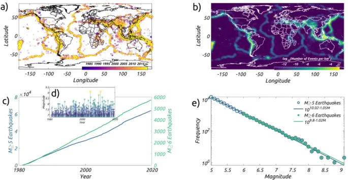
waves, electric potential differences, ground water chemistry etc) are effectively left out since they cannot be adequately
51
tested in the provided CSEP framework. Recent studies have also pointed out deficiencies that introduce biases against
52
models that do not share the assumptions of the CSEP testing methodology. Moreover, some researchers have expressed
53
concerns regarding the effective public communication of the numerous test results associated with each model. Some
54
have argued that test metrics should be tailored not only to the small community of highly-sophisticated statistical
55
seismologists, but to the intuitive understanding of the general public and civil protection agencies.
56
We suggest that the drawbacks and limitations of the previous testing methodologies can be addressed by establishing a
57
real-time global earthquake forecasting model that serves as a benchmark for evaluating not only grid based seismicity
58
rate models but also a wide variety of alarm based methods. We thus introduced RichterX: a global earthquake
59
prediction platform where participants can query the probability of an earthquake (or a number of earthquakes) above a
60
given magnitude to occur in a specific time-space window, and issue to-occur or not-to-occur predictions [Kamer et al.,
61
2020]. By analyzing the prospective outcomes of the issued predictions we can establish if they exhibit significant skill
62
compared to our global reference model, and if they do, we can successfully rank them accordingly.
63
This work documents the development of such a global earthquake forecasting model derived from the Epidemic
64
Type Aftershock Sequence (ETAS) family and presents a novel set of rigorous tests tailored to the specific needs
65
of short term earthquake forecasting and benchmarking of short term earthquake predictions. ETAS based models
66
have been shown to be the best contenders in the horse race organised within CSEP. Moreover, they contain generic
67
and parsimonious assumptions that provide consistent descriptions of the statistical properties of realised seismicity.
68
Specifically, the ETAS family of models is based on the following assumptions: (i) the distinction between foreshocks,
69
mainshocks and aftershocks is artificial and all earthquakes obey the same empirical laws describing their probability to
70
occur and their ability to trigger future earthquakes; (ii) earthquakes have their magnitude distributed according to the
71
Gutenberg-Richter distribution; (iii) the rate of triggered events by a given earthquake obeys the Omori-Utsu temporal
72
law of aftershocks; (iv) the number of earthquakes triggered by a given event obeys a productivity law usually linking
73
the average number of offsprings to the exponential of the triggering earthquake magnitude; (v) triggered events are
74
distributed in space according to a spatially dependent power law function.
75
Here, we develop horse races between two ETAS models differing in their specification of their time kernels, one with
76
an exponentially tapered Omori kernel (ETOK) and another with a magnitude dependent Omori kernel (MDOK). We
77
define three different training settings for the auxiliary catalog’s magnitude cutoff (3, 4 or 5) and two different training
78
settings for the primary catalog’s magnitude cutoff (5 or 6), in 362 pseudo prospective global experiments designed to
79
forecastM ≥5andM ≥6earthquakes at three different spatial resolutions, spanning scales from45kmto180km.
80
While previous works have shown the importance of accounting for spatially varying ETAS parameters [Nandan et al.,
81
2017], here we assume the same ETAS parameters hold for the whole Earth. This assumption is made for computational
82
simplicity and with the intention to have a uniform global reference model allowing for an easier interpretation of the
83
participants’ predictive performance. This also allows us to focus on the key question we want to investigate, namely
84
the role of a possibly magnitude dependent Omori exponent on forecasting skills. This hypothesis has been derived
85
from a physics-based model of triggered seismicity based on the premises that 1) there is an exponential dependence
86
between seismic rupture and local stress and 2) the stress relaxation has a long memory [Ouillon and Sornette, 2005;
87
Sornette and Ouillon, 2005]. These physical ingredients predict that the exponent of the Omori law for triggered events
88
is an increasing function of the magnitude of the triggering event. This prediction has been corroborated by systematic
89
empirical studies for California and worldwide catalogues [Ouillon and Sornette, 2005], as well as for Taiwanese [Tsai
90
et al., 2012] and Japanese [Ouillon et al., 2009] catalogues.
91
Therefore we consider the addition of magnitude dependant Omori law as a potential improvement to a global
92
implementation of the ETAS model. We propose a general pseudo-prospective testing experiment that can be applied to
93
any future candidate model. The testing experiment is designed to address the specific needs of a global, short-term
94
earthquake forecasting application and correct for some of the defects highlighted by our previous work [Nandan et al.,
95
2019c,b]. In particular, we use equal sized meshes compatible with the spatial scales available on the RichterX platform
96
(radius in the range of 30-300km) and target duration of 30 days, which is the maximum prediction time window in
97
RichterX.
98
The organisation of the paper is as follows. Section 2 presents the data used in our tests and its main properties. Section
99
3 starts with a description of the pseudo-prospective forecasting experiments. Then, it defines the two ETAS models that
100
are compared. We explain how parameters inversion is performed and the details of the simulations used to construct
101
the forecasts. Section 4 presents the results, starting with a rate map and full distributions of earthquake numbers in the
102
different cells covering the Earth at the eleven different resolution levels. The model comparisons are performed in
103
terms of pair-wise cumulative information gains, and we calculate the statistical significance of right tailed paired t-tests.
104
We study in details the sensitivity of our results to the spatial resolution, number of simulations and inclusion of smaller
105
magnitudes in the auxiliary catalogs. We also describe how the best performing model is adopted as a benchmark for
106
the RichterX global earthquake prediction contest, which is presented in more details in a companion paper. Section 5
107
concludes by summarising and outlining further developments. A supplementary material document provides additional
108
figures and descriptions for the interested readers.
109
2 Data
110
We use the global earthquake catalog obtained from the Advanced National Seismic System (ANSS) database. To
111
maintain the same precision for all reported earthquakes in the catalog, we first bin the reported magnitudes at 0.1 units.
112
In this study, we use allM ≥5earthquakes that occurred between January 1981 and October 2019 as our primary data
113
source for target earthquakes.
114
Figure 1 shows the different features of this dataset. In Figure 1a we show the location, time and magnitudes of these
115
earthquakes. Figure 1b shows the spatial density ofM ≥ 5earthquakes. This spatial density is obtained by first
116
counting the number of earthquakes in1×1deg2pixels, normalizing the counts by the area of each pixel and then
117
smoothing the resultant density. We also show the time series of cumulative number ofM ≥5andM ≥6earthquakes
118
and the magnitudes vs. times ofM ≥7earthquakes in Figures 1c and 1d, respectively.
119
Finally, in Figure 1e, we show the empirical magnitude distribution ofM ≥5andM ≥6earthquakes. To each of
120
them, we separately fit the Gutenberg-Richter(GR) law. The maximum likelihood estimate of the parameters of the GR
121
distribution forM ≥5andM ≥6earthquakes are indicated in the inset in figure 1e. In order of obtain the exponent
122
of the GR distribution, we use the analytical maximum likelihood estimator for binned magnitude derived by Tinti and
123
Mulargia [1987]. Having obtained the exponent, the prefactor of the GR distribution can be analytically estimated. The
124
GR law exponents obtained for both magnitude thresholds are1.05(M ≥5) and1.02(M ≥6) and are thus nearly
125
identical. Such consistency is often treated as an indication of the completeness of the catalog [Cao and Gao, 2002;
126
Mignan and Woessner, 2012]. With this reasoning, the consistency of GR exponents indicates the completeness of the
127
catalog forM ≥5in our case.
128
For the appropriate calibration of the ETAS model, we also use theM ≥3earthquakes between January 1975 and
129
October 2019 as auxiliary dataset. The use of auxiliary dataset is often encouraged in ETAS literature [Schoenberg
130
et al., 2010; Wang et al., 2010; Seif et al., 2017], as it allows to minimize the biases in the genealogy tree of earthquakes
131
due to the missing sources [Sornette and Werner, 2005a]. Earthquakes in the auxiliary catalogs can act only as sources
132
during the calibration of the ETAS model, thus, their completeness is not required.
133
For the sake of reproducibility, since catalogs are subject to updates, the catalog used in this study is provided as a
134
supplementary material.
Figure 1: Features of primary data used in this study; (a) Location ofM ≥ 5 earthquakes since 1981; Sizes of the earthquakes scale with their magnitude and colors show the year of occurrence; (b) Spatial density ofM ≥5 earthquakes since 1981 obtained by smoothing the counts of earthquakes in1×1deg2grid with a Gaussian filter; (c) Cumulative number ofM ≥5andM ≥6earthquakes, with their respective scaled axes on the left and right side of the plot, respectively; (d) Magnitude vs. Time plot ofM ≥7earthquakes; (e) Empirical frequency magnitude distribution ofM ≥5andM ≥6earthquakes; Lines show the best fit Gutenberg Richter Distribution to the empirical distribution ofM ≥5andM ≥6earthquakes.
135
3 Method
136
In this study, our aim is to compare the performance of different models (described in Section 3.2) in forecasting future
137
earthquakes. We do this by means of pseudo prospective experiments.
138
3.1 Pseudo Prospective Forecasting Experiments
139
Prospective forecasting experiments are a powerful tool allowing scientists to check if the improvements lead to better
140
forecasts of future unseen observations. Truly prospective experiments are time consuming, as they require many years
141
before enough future observations accumulate to strengthen (or weaken) the evidence in favor of a model [Kossobokov,
142
2013]. A practical solution is to conduct pseudo prospective experiments. In these experiments, one uses only the early
143
part of the dataset for the calibration of the models and leaves the rest as virtually unseen future data. Subsequently, the
144
calibrated models are used to simulate a forecast of future observations and the left out data is used to obtain a score for
145
each of the forecasting models. These scores can then be compared to identify the best model.
146
Although, (pseudo) prospective experiments have started to catch up in the field of earthquake research [Kagan and
147
Jackson, 2010; Zechar and Jordan, 2010; Eberhard et al., 2012; Kagan and Jackson, 2011; Zechar et al., 2013; Ogata
148
et al., 2013; Hiemer et al., 2014; Hiemer and Kamer, 2016; Schorlemmer et al., 2018; Nandan et al., 2019b,c], they still
149
have not become the norm. In this regard, the work done by the collaboratory for the study of earthquake predicatbility
150
(CSEP) and others [Schorlemmer et al., 2018; Kossobokov, 2013] has been very commendable, as they have tried to
151
bring the prospective model validation on the center stage of earthquake forecasting research. However, the prescribed
152
prospective validation settings, in particular by CSEP, are too primitive and sometimes biased in favour of certain
153
model types. For instance, most of the CSEP experiments have been conducted with spatial grids which are defined as
154
0.1×0.1deg2cells (see for instance Zechar et al. [2013]) or0.05×0.05deg2cells (e.g. Cattania et al. [2018]), mostly
155
for computational convenience. However, as the area of these cells vary with latitude, becoming smaller as one moves
156
north or south from the equator, a model gets evaluated at different spatial resolutions at different latitudes, thus, by
157
construction, yielding different performances as a function of latitude. This areal effect on the performance then gets
158
convoluted with the underlying spatial variation in the performance of the model. For instance, modelers might find that
159
their models yield better performance in California, but very poor performance in Indonesia at a fixed spatial resolution.
160
Should they then infer that their models are better suited for a strike slip regime than for a subduction setting? Due to
161
the inherent nature of the varying spatial resolution of the grid prescribed by CSEP, the answer to this question becomes
162
obfuscated.
163
Another aspect of pseudo prospective experiments that is poorly handled by CSEP is that it forces the modelers to
164
assume Poissonian rates in a given space-time-magnitude window irrespective of their best judgement. Nandan et al.
165
[2019b] showed that this choice puts the models that do not comply with the Poissonian assumption on weaker footing
166
than those models which agree with this assumption. As a result, the reliability of the relative rankings obtained from
167
the models evaluated by CSEP remains questionable to some extent.
168
Last but not the least, in some model evaluation categories [Werner et al., 2011; Schorlemmer and Gerstenberger, 2007],
169
CSEP evaluates the models using only "background" earthquakes, which are identified using Reasenberg’s declustering
170
algorithm as being independent [Reasenberg, 1985]. However, as the earthquakes do not naturally come with labels
171
such as "background", "aftershocks" and "foreshocks" that can be used for validation, this a posteriori identification
172
remains highly subjective. In regards to CSEP’s use of the Reasenberg’s declustering algorithm, Nandan et al. [2019c]
173
pointed out that the subjective nature of declustering introduces a bias towards models that are consistent with the
174
declustering technique, rather than the observed earthquakes as a whole. This puts into questions the value of such
175
experiments, as their results are subject to change as a function of the declustering parameters.
176
Since the aim of our forecasting experiment is to assess which model is more suitable to serve as a reference model for
177
the global earthquake prediction platform RichterX, it becomes important to address the drawbacks mentioned above by
178
designing a testing framework tailored to multi-resolution, short-term forecasts on a global scale. Accordingly we have
179
designed the pseudo prospective experiments in this study with the following settings:
180
1. Many training and testing periods: We start testing models beginning on January 1, 1990 and continue
181
testing till October 31, 2019, spanning a duration of nearly 30 years. The maximum duration of an earthquake
182
prediction that can be submitted on the RichterX platform is 30 days. Using this time window, our pseudo
183
prospective experiments are composed of 362 non overlapping, 30 days long testing periods. To create the
184
forecast for each of the testing periods, the models are calibrated only on data prior to the beginning of each
185
testing period for calibration as well as simulation. The forecasts are specified on an equal area mesh with
186
predefined spatial resolution.
187
2. Equal area mesh:To create this equal area mesh, we tile the whole globe with spherical triangles whose area
188
is constant all over the globe. This mesh is designed in a hierarchical fashion. To create a higher resolution
189
mesh from a lower resolution one, the triangles in the lower resolution mesh are divided into four equal area
190
triangles. In this way, we create eleven levels of resolution: at the first level, the globe is tiled with20equal
191
area triangles (corresponding to an areal resolution of≈25.5×10⁶km2each); at the second level 80 equal
192
area triangles tile the globe, and so on. Finally, at level eleven≈21×106triangles tile the globe with an areal
193
resolution of≈24km2. In this study, we evaluate the models at level six (unless otherwise stated), which
194
has an areal resolution equivalent to a circle with radius≈90km. To test the sensitivity of our results to the
195
choice of areal resolution, we also evaluate the models at level five and level seven, which correspond to an
196
areal resolution equivalent to circles with radii≈180kmand≈45km, respectively. In principle, the models
197
can be evaluated at all spatial resolutions (from 1 to 11). The resolutions in this study are chosen to be in
198
accordance with the the spatial extents used on the RichterX platform (radius of 30 to 300km).
199
3. Flexibility to use parametric or non-parametric probability distributions:The model forecasts can be
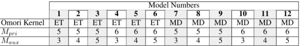
200
specified on the equal area mesh during each testing period either as the full distribution of earthquake numbers
201
(as in Nandan et al. [2019b]) empirically obtained from the simulations, or as a Poissonian rate or as any other
202
analytical probability distribution function that may be in line with the model assumptions.
203
4. Performance evaluation using all earthquakes withM ≥5orM ≥6:We test the models against target
204
sets consisting ofM ≥5andM ≥6events that occurred during each testing period. During a given testing
205
period, competing models forecast a distribution of earthquake numbers (M ≥5orM ≥6depending on
206
the choice of target magnitude threshold orMt) in each triangular pixel. We then count the actual number of
207
observed earthquakes in each pixel. With these two pieces of information, the log likelihoodLLiAof a given
208
model A during theithtesting period is defined as:
209
LLiA=
N
X
j=1
ln(P rij(nij) ) (1)
whereP rijis the probability density function (PDF) of earthquake numbers forecasted by model A andnij
210
is the observed number of earthquakes (≥Mt) during theithtesting period in thejthpixel.N is the total
211
number of pixels, which at level six is equal to 20,480. Similarly,LLiBfor another competing model (B) can
212
be obtained. The information gainIGiABof model A over model B for theithtesting period is equal to
213
IGiAB=LLiA−LLiB . (2)
In order to ascertain if the information gain of model A over B is statistically significant over all testing periods,
214
we conduct a right tailed paired t-test, in which we test the null hypothesis that the mean information gain
215
(M IGAB=
P
iIGiAB
362 ) over all testing periods is equal to 0 against the alternative that it is larger than 0. We
216
then report thep-values obtained from the test. If thep-values obtained from the tests are smaller than the
217
"standard" statistical significance threshold of 0.05, model A is considered to be statistically significantly more
218
informative than model B.
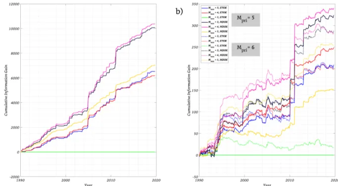
219
3.2 Competing Models
220
3.2.1 Preliminaries on ETAS models
221
In this study, we conduct a contest between different variants of ETAS models only. The reasons for this are multifold:
222
1. Our target use case for RichterX requires providing near-real time short time earthquake forecasts on a global
223
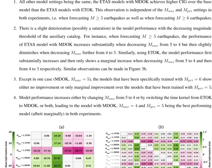
scale. ETAS models are suitable for such applications as they rely only on a timely stream of earthquake
224
locations and magnitudes, whereas models based on stress transfer require additional data, such as fault plane
225
orientations, rupture extent, slip distributions etc. which are often available only after a few days.
226
2. Due to the abundance of target events (the world-wide average number ofM ≥5andM ≥6earthquakes
227
per month, since 1990, is≈137and≈13, respectively), global models providing short term (here, monthly)
228
earthquake forecasts can be tested with a greater statistical significance (even at high magnitude threshold,
229
such asM ≥5andM ≥6, of the testing catalog), compared to their regional counterparts.
230
3. On the global scale, there exist some "long term" models [Bird et al., 2015; Kagan and Jackson, 2011, 2010].
231
However, there is no model (to the best of our knowledge) that provides short term forecasts. We intend to fill
232
this gap with the best performing ETAS model of this study.
233
4. On the regional scale, ETAS models [Nandan et al., 2019c] have been shown to be much more effective than
234
standard smoothed seismicity models [Werner et al., 2011; Helmstetter et al., 2006], which provide forecasts
235
of future earthquakes by smoothing the location of past background earthquakes. However, their forecasting
236
effectiveness on the global scale remains to be assessed.
237
In this study, our goal is not to provide a comprehensive test between various types of state-of-the-art forecasting
238
approaches [Bach and Hainzl, 2012; Helmstetter and Werner, 2014; Gerstenberger et al., 2005; Steacy et al., 2014;
239
Reverso et al., 2018; Cattania et al., 2014, 2018], but rather to design an experiment in which short term global
240
earthquake forecasting models can be developed, compared and enhanced. Furthermore, we only conduct the horse race
241
between the simplest ETAS models. This means that we exclude space and time variation of its parameters, which
242
have been actively reported by numerous authors, at regional and global scales [Page et al., 2016; Zhang et al., 2020;
243
Chu et al., 2011; Nandan et al., 2017; Ogata, 2011], to lead to enhanced performance. Furthermore, the ETAS models
244
considered in this study do not make use of any other datasets such as fault networks, global strain rates, source models,
245
focal mechanisms and so on. Some authors [Cattania et al., 2018; Guo et al., 2015; Bach and Hainzl, 2012] have shown
246
in case studies that these additional datasets enhance the forecasting potential of ETAS type models. We disregard these
247
complexities, not due to any underlying belief that they are not informative, but because their limited availability would
248
hinder a real-time implementation on the RichterX platform. We also maintain that the initial model should be simple
249
enough. Then, adding complexities should follow sequentially, only if they can be justified by their forecasting gains
250
over simpler models. With these points in mind, in the following, we describe the different variants of ETAS models
251
that we have compared in this study.
252
3.2.2 ETAS model with exponentially tapered Omori kernel (ETOK)
253
Model Description In this model, the seismicity rateλ(t, x, y|Ht)at any timetand location(x, y)depends on the
254
history of the seismicityHtup totin the following way:
255
λ(t, x, y|Ht) =µ+ X
i:ti<t
g(t−ti, x−xi, y−yi, Mi) (3)
whereµis the time-independent background intensity function,gis the triggering function and(ti, xi, yi, Mi)represents
256
the time, x-coordinate, y-coordinate and magnitude of theithearthquake in the catalog, respectively.
257
The memory functiongin Equation 3 is formulated as:
258
g(t−ti, x−xi, y−yi, Mi) =Kea(Mi−Mc)× e−t−τti (t−ti+c)1+ω
×h
(x−xi)2+ (y−yi)2+deγ(Mi−Mc)i−1−ρ (4) which is the product of three kernels:
259
1. The productivity kernelKea(Mi−Mc)quantifies the expected number of aftershocks triggered by an earthquake
260
with magnitudeMiabove the magnitude of completeness,Mc, whereKandaare the productivity constant
261
and exponent respectively.
262
2. The exponentially tapered Omori kernel e−
t−ti τ
(t−ti+c)1+ω quantifies the time distribution of the direct aftershocks
263
of an earthquake that occurred atti. The exponential taper terme−t−τti ensures that the parameterωcan
264
attain even negative values during the calibration of the model, which is not possible for a pure power law
265
distribution, as it becomes unnormalizable for exponents smaller than 1.
266
3. The isotropic power-law spatial kernel
(x−xi)2+ (y−yi)2+deγ(Mi−Mc)−1−ρ
quantifies the spatial
267
distribution of the aftershocks of an earthquake with magnitudeMithat occurred at(xi, yi).
268
Note that the model defined in Equations 3 and 4 implicitly assumes that the magnitudes of both the background and the
269
triggered earthquakes follow the Gutenberg Richter (GR) distribution, which is described by the following probability
270
density function (PDF):
271
f(M) =βe−β(M−Mc) (5)
Note that the exponentβ in expression (5) is related to the b-value reported above in the inset of Figure 1e via
272
β =bln 10≈ 2.3b. Thus a value ofβin the range 2.3-2.4 as shown in Figure S1 in the supplementary materials
273
corresponds to a b-value in the range 1.0-1.04.
274
Due to its commonality in both the background and the triggering function, GR law is usually factored out of the
275
explicit formulation of the ETAS model. However, one could imagine other formulations of ETAS models in which
276
such factoring out is not possible. For instance, simply allowing the background earthquakes and aftershocks to follow
277
GR distribution with different exponents (β1andβ2) makes the factoring impossible and the exponentsβ1andβ2then
278
have to be jointly inverted with the other ETAS parameters. In this context, Nandan et al. [2019a] showed that, using
279
the Californian earthquake catalog, not only the exponents corresponding to the background earthquakes are distinct
280
from those of aftershocks, but also that the magnitude distribution of direct aftershocks is scaled by the magnitude
281
of their mainshock. Despite these findings, we make the simplifying assumption that both background earthquakes
282
and aftershocks follow the same GR distribution, and factor it out from the explicit formulation of the ETAS model.
283
Nevertheless, the GR law plays an explicit role when the ETAS model is used to forecast the magnitude of the future
284
earthquakes and its parameterβhas thus to be inverted from the training period.
285
Simulation We follow the standard algorithms for the simulation of synthetic earthquake catalogs for the ETAS
286
model [Zhuang et al., 2004, 2002; Nandan et al., 2019b]. For completeness, a detailed description of the simulation is
287
also provided in the Supplementary Text S1.
288
Parameter Inversion And Modelling Choices As described in Supplementary Text S1, the set of parameters
289
{µ, K, a, c, ω, τ, d, ρ, γ, β} are necessary for the simulation of future earthquake catalogs. The values of these
290
parameters are not known in practice and they have to be inverted from the training data. The parameters
291
{µ, K, a, c, ω, τ, d, ρ, γ} can be inverted by calibrating the model (Equation 3) on the real data by means of the
292
Expectation Maximization (EM) algorithm proposed by Veen and Schoenberg [2008]. To obtain the parameterβ, we
293
first bin the magnitudes of the earthquakes in the ANSS catalog in 0.1 units and then use the analytical maximum
294
likelihood estimator derived by Tinti and Mulargia [1987] for binned magnitudes.
295
An important consideration before calibrating the ETAS model is the choice of the primary and auxiliary catalogs.
296
The main difference between these two catalogs is that earthquakes in the primary catalog can act both as targets and
297
sources during the calibration of the ETAS model, while the earthquakes in the auxiliary catalogs can act only as
298
sources. In ETAS literature [Schoenberg et al., 2010; Wang et al., 2010; Seif et al., 2017], the use of auxiliary catalogs
299
is encouraged during inversion of ETAS parameters, so as to minimize the biases in the genealogy tree of earthquakes
300
due to the missing sources [Sornette and Werner, 2005a; Saichev and Sornette, 2006b]. In this study, we calibrate
301
the ETAS model (described in Equations 3 and 4) using primary catalogs with two different magnitude thresholds:
302
Mpri =5 and 6. Both these primary catalogs start in year 1981 and include earthquakes from all over the globe. For
303
the auxiliary catalogs, which start in 1975 and are also composed of earthquakes from all over the globe, we use three
304
different magnitude thresholds:Maux=3, 4 and 5 during calibration. We use different magnitude thresholds for the
305
primary catalogs to test the hypothesis that better forecasting potential can be achieved for higher magnitude thresholds
306
if we specifically train our models for them. We use different magnitude thresholds for the auxiliary catalog to test the
307
hypothesis that smaller earthquakes play an important role in triggering and can improve the forecasting potential of the
308
ETAS models.
309
Note that, even though the available ANSS catalog extends down to magnitude 0, we do not use such a low magnitude
310
threshold for the auxiliary and the primary catalogs because: (1) in the formulation of the ETAS model, the primary
311
catalog should follow a GR law and be complete above the considered threshold magnitude. These two criteria can not
312
be fulfilled for the global ANSS catalog at magnitude thresholds lower than 5, and extending back to year 1981; (2)
313
lowering the magnitude threshold of both the primary and auxiliary catalog increases enormously the computational
314
burden for both the inversion and simulations.
315
In Figure S2, we show the time evolution of the estimates of the parameters for the ETAS model with exponentially
316
tapered kernel forMaux=3, 4 and 5 andMpri=5 . The time evolution forMpri =6, for the same model and the
317
three auxiliary magnitude settings, is shown in Figure S3. Beside the "usual" ETAS parameters, Figure S2 shows
318
the time series of the branching ratio. This parameter quantifies the average number of triggered earthquakes of first
319
generation per triggering event, as well as the fraction of triggered earthquakes in the training catalog [Helmstetter
320
and Sornette, 2003]. For a branching ratio<1, the system is in the the sub-critical regime. For a branching ratio>1,
321
the system is in the super-critical regime [Helmstetter and Sornette, 2002]. In addition, in Figure S1, we show the
322
time evolution of the parameterβfor twoMpri settings. Since the parameterβ is only estimated from the primary
323
catalog, only two time series are obtained and not six (one for each of the twoMprisettings) as in the case of other
324
ETAS parameters. The time series of all the parameters is composed of 362 points, each corresponding to one of the
325
training catalogs preceding the 362 testing periods. We notice that parameters show conspicuous variation with time,
326
with a tendency to stabilise after about 2011, perhaps reflecting a better global catalogue completeness. We cannot
327
exclude a genuine trend resulting from the shortness of the time series, which are strongly impacted by the two great
328
earthquakes of magnitude larger than 9 that occurred in 2004 (great Indian ocean earthquake) and 2011 (Tohoku, Japan).
329
Furthermore, some of the parameter pairs (µ,nor branching ratio), (c,ω) and so on exhibit cross correlations. In
330
addition, the parameters also seem to be systematically dependent on the choices ofMauxandMpri. Investigating the
331
sources of these time variations, cross correlations and dependencies on auxiliary and primary magnitude thresholds is
332
beyond the scope of this paper. In this article, we focus on evaluating the importance of these hyper-parameter choices
333
(MauxandMpri) in terms of forecasting performance. Nevertheless, we report the time evolution of these parameter
334
estimates as it would aid the readers in reproducing the results presented in later sections.
335
3.2.3 ETAS Model With Magnitude Dependent Omori Kernel (MDOK)
336
Model Description While the primary equation of the seismicity rate for this ETAS model remains the same (Equation
337
3), the triggering kernel is modified to account for a possible magnitude dependence of Omori-Utsu parameterscandω.
338
The triggering kernel for this model is redefined as:
339
g(t−ti, x−xi, y−yi, Mi) =Kea(Mi−Mc)× e−t−τti
[t−ti+c(Mi)]1+ω(Mi)
×h
(x−xi)2+ (y−yi)2+deγ(Mi−Mc)i−1−ρ
(6)
wherec(Mi) = 10c0+c1Miandω=ω0+ω1Mi.
340
The functional form forc(M)is inspired from the works of Shcherbakov et al. [2004], Davidsen et al. [2015] and
341
Hainzl [2016a]. All three authors found the c-value to increase exponentially with the mainshock magnitude. While the
342
first two authors interpreted the c-value dependence on the mainshock magnitude as a part of a self-similar earthquake
343
generation process (i.e. a physical process), Hainzl [2016a] attributed this dependence to the rate dependent aftershock
344
incompleteness (i.e. a data sampling issue). The latter would require to replace the missing events in some way, as they
345
play a role in triggering of future events. Yet no such procedure has ever been proposed. Note that several other authors
346
[Scholz, 1968; Dieterich, 1994; Narteau et al., 2005] have also argued for the magnitude-dependence of the onset of the
347
power-law decay based on ideas such as stress corrosion and rate and state dependent friction. However, these authors
348
suggest that the c-value would correlate negatively with mainshock magnitude, as their model predicts that the larger
349
the stress perturbation, the shorter would be the duration between the mainshock and the onset of the power-law decay.
350
Regardless of the underlying mechanism for the dependence of the c-value on mainshock magnitude, the evidence for
351
such an exponential dependence is rather clear, and thus warrants an explicit formulation within the ETAS model.
352
The linear dependence of the Omori exponentωon the mainshock magnitude is based on the work of Ouillon and
353
Sornette [2005] and Sornette and Ouillon [2005], who reported strong empirical evidence together with a physics-based
354
theory for such a dependence for mainshocks in Californian and worldwide catalogs. Tsai et al. [2012] confirmed
355
this observation for the Taiwanese catalog and Ouillon et al. [2009] for the Japanese catalog. These authors used a
356
wealth of different techniques, such as various space-time windowing methods, binned aftershock time-series, wavelet
357
analysis and time evolution of aftershocks maximum magnitude, in order to ascertain the robustness of the results and
358
that the observed magnitude dependence ofωwould not be due to some bias induced by a specific method. Ouillon
359
and Sornette [2005] and Sornette and Ouillon [2005] proposed a theoretical statistical physics framework in which the
360
seismic rate results from an exponential Arrhenius like activation with an energy barrier influenced by the total stress
361
fields induced by past earthquakes and far-field tectonic loading. These authors showed that the combination of the
362
exponential activation rate together with the long memory kernel of stress relaxation leads to temporal multifractality
363
expressed empirically as a magnitude-dependent Omori exponentω. They coined this model the multifractal stress
364
activation (MSA) model. More precisely, the MSA model can be rationalized as follows:
365
1. the stress at any location is the sum of the far-field contribution due to tectonic loading and the stress fluctuations
366
due to past events;
367
2. each earthquake ruptures a complex set of patches whose number increases exponentially with the magnitude
368
of the event;
369
3. each failing patch redistributes stress in its surrounding according to the laws of linear elasticity, so that
370
positive or negative stress contributions add up as patches fail and consecutive earthquakes occur. The stress
371
transferred by a failed patch at any target location can be treated as a random variable distributed according
372
to a Cauchy law, i.e., decaying as a power law with exponent(1 +ν)/2[Kagan, 1992]. The effect of the
373
earthquake rupture at the target location is thus the sum of the corresponding random variables. The exponent
374
νthus encompasses all the geometrical complexity of the problem: the (fractal) nature of the fault system, the
375
Gutenberg–Richter law (i.e., the size of the source events), the distribution of focal mechanisms, the (possibly
376
self-affine) morphology of slip along the rupture plane, and the spatial decay of the stress Green’s function;
377
4. the memory of local past stress fluctuations decays as a power-law of time, due to rock (nonlinear) viscosity,
378
with exponent1+θ. This function encapsulates all brittle and ductile relaxation phenomena such as dislocations
379
motion, pressure-dissolution, slow earthquakes or even those too small to be detected. In that sense, θ
380
characterizes the whole complexity of stress relaxation in the crust.
381
5. at any location, the seismicity rate depends exponentially on the local shear stress, in agreement with many
382
known underlying failure processes;
383
The model then predicts that the seismicity rate consists in a time invariant base rate due to the tectonic loading,
384
nonlinearly modulated by a time varying term depending on past seismicity. This term can increase the rate if past
385
(and/or most recent) stress fluctuations are positive, but may also decrease if they are negative. When solved self-
386
consistently by considering all (statistical) mechanical interactions between events, the model predicts that the Omori
387
exponent of the triggered sequence following an event of magnitudeM decays with time with an exponentpincreasing
388
linearly withM. This peculiar feature is indeed predicted to hold exactly when the conditionν(1 +θ) = 1is fulfilled,
389
which can be viewed as the consequence of the space-time self-organization of fault networks in the brittle crust.
390
Reviewing the possible values of parametersν andθfor the Earth’s crust, Ouillon et al. [2009] showed that their
391
estimations allowed them to bracket this criterion, thus evidencing another analogy with second-order phase transitions
392
where critical exponents are linked by such relationships close to a critical point.
393
In this forecasting experiment, we aim to systematically test the idea that explicitly taking account of magnitude
394
dependence in these two Omori parameters would lead to an improvement in the forecasting ability of the modified
395
ETAS models relative to the ones in which these dependencies are ignored.
396
Simulation Given the set of parameters{µ, K, a, c0, c1, ω0, ω1, τ, d, ρ, γ, β}, the simulation of the time, location and
397
magnitude of the future earthquakes proceed in the same way as for a standard ETAS model (see Supplementary Text
398
S1), except for one difference. In this case, the times of the direct aftershocks of an earthquake with magnitudeMi 399
are simulated using the time kernel whose parameters depend onMiin the way described in Equation 6. This means
400
that, despite the fact that the MSA model is by construction nonlinear, we here consider a linear approximation for the
401
purpose of tractability. Indeed, in the MSA model, the exponential nonlinearity occurs in the stress space, a variable
402
that is not computed within the ETAS formulation which focuses only on rates. A full MSA approach would require to
403
compute the stress transfer (and its time dependence) due to all past events, taking account of their individual rupture
404
complexity, and assessing all their uncertainties. As this remains challenging in the present state of seismological
405
research, we bypass this obstacle and provide a simplified approach by introducing a magnitude-dependent Omori
406
kernel.
407
Parameter Inversion And Modelling Choices Again in this case, we adapt the EM algorithm proposed by Veen and
408
Schoenberg [2008] to invert the parameters of the model (Equation 6). For the sake of completeness, we also calibrate
409
these models with six primary and auxiliary catalog settings as described in Section 3.2.2. Again, without going into
410
the possible underlying causes of the time variation of the estimated parameters and their dependence on the choice
411
ofMauxandMprihyper-paramters, we report the time evolution of the estimated parameters for ETAS model with
412
magnitude dependent Omori kernel in figures S4 and S5.
413
3.3 Summary of competing models and experiment settings
414
In summary, we have twelve competing models: six models belong to the ETOK class and six belong to the MDOK
415
class. In each of these two classes, three models are calibrated with a primary catalog magnitude thresholdMpri= 5
416
and three others are calibrated with a thresholdMpri = 6. These three models can be distinguished based on the
417
different magnitude thresholds for the auxiliary catalog,Maux= 3,Maux = 4andMaux= 5, used during calibration
418
and simulations.
419
Each of these twelve models are shown in Table 1 and are individually calibrated on the 362 training period periods.
420
We then compare their forecasting performance using theM ≥5andM ≥6earthquakes under the validation settings
421
prescribed in Section 3.1. Only models that have been been calibrated withMpri = 5are used to forecastM ≥5
422
earthquakes to avoid "extrapolated" forecasts of models trained with onlyM ≥6earthquakes. All the models are used
423
to forecast theM ≥6earthquakes as targets during each 30 days long validation period. In summary, six models
424
are validated and scored usingM ≥5earthquakes and all the twelve models are validated and scored usingM ≥6
425
earthquakes.
426
Figure2:(a)TotalRateofM≥5earthquakes(km−2month−1)between12/03/2011and11/04/2011forecastedusingETASmodelwithMDOK,Maux=4and Mpri=5;TheMw9.1Tohukuearthquakeoccurredon11/03/2011;(b-d)Ratesofthreetypesofearthquakes(seeSectionS1)thataresuperposedtocreatethefinal forecastshowninpanela;(b)backgroundevents;(c)aftershocksoftype1;(d)aftershocksoftype2;theaveragenumberofeachearthquaketypeinthefinalforecast isindicatedinpanelsb-d;(e-l)Probabilitydensityfunctions(PDF)ofearthquakenumbersthatareforecastedbythemodelinthecirculargeographicregionofradius =300kmaround“earthquakeprone”citiesoftheworld.
Model Numbers
1 2 3 4 5 6 7 8 9 10 11 12
Omori Kernel ET ET ET ET ET ET MD MD MD MD MD MD
Mpri 5 5 5 6 6 6 5 5 5 6 6 6
Maux 3 4 5 3 4 5 3 4 5 3 4 5
Table 1: All twelve models resulting from different calibration choices; ET and MD stand for ETAS models with exponentially tapered Omori kernel and magnitude dependent Omori kernels, respectively.
4 Results and Discussion
427
4.1 Forecasted Rate Map And Full Distribution Of Earthquake Numbers
428
In this section, we illustrate how the forecasts of different models are constructed. We do this only for a selected model
429
and a particular testing period, as the procedure for all other testing periods and models is the same.
430
Figure 2(a) shows the net forecasted rate of earthquakes (perkm2per month) in the time period immediately following
431
the Tohoku earthquake (between 12/03/2011 and 11/04/2011) for the ETAS model with magnitude dependent Omori
432
kernel (MDOK) and auxiliary magnitude setting ofMaux= 4and primary magnitude setting ofMpri= 5. Figures 2(b-
433
d) show the contributions of the three type of earthquakes to the net forecasted rate. The first contribution comes from
434
the background earthquakes that are expected to occur during the testing period (Figure 2b). The second contribution is
435
from the cascade of aftershocks (Aftershock Type 1) that are expected to be triggered by the earthquakes in the training
436
period (Figure 2c). The third and the final contribution comes from the cascade of aftershocks (Aftershock Type 2)
437
that are expected to be triggered by the background earthquakes occurring during the testing period (Figure 2d). In
438
this particular testing period, the Type 1 aftershocks have the highest contribution, with≈264 earthquakes on average,
439
while the contributions of the background earthquakes and Type 2 aftershocks are relatively minuscule. The occurrence
440
of the Tohoku earthquake just before the testing period is the main cause of this dominance. However, it is important to
441
note that the relative importance of these three components depends on the time scale of the testing period. For longer
442
testing periods, such as on the order of a decade to a century, the contribution of background earthquakes and especially
443
of Type 2 aftershocks becomes significant, if not dominating compared to the Type 1 aftershocks.
444
It is important to mention here that these average rate maps are just used for the sake of illustration of the generated
445
forecasts, as they provide a convenient representation. In reality, each pixel on the globe is associated with a full
446
distribution of forecasted earthquake numbers. To illustrate this, we show in Figure 2 (e-l) the probability density
447
function (PDF) of earthquake numbers that is forecasted by the model in circular geographic regions (with 300 km
448
radii) around some of the “earthquake prone” cities of the world. These PDFs are obtained by counting the number of
449
simulations in which a certain number of earthquakes were observed and then by dividing those by the total number of
450
simulations that were performed. In this study, we perform 100,000 simulations for all the models and for all testing
451
periods. Notice that the PDF of the forecasted number of earthquakes varies significantly from one city to another,
452
despite the fact that none of the competing models feature spatial variation of the ETAS parameters. This variation can
453
be attributed to variation in the local history of seismicity from one place to another. Other factors that control the shape
454
of these distributions include the time duration of the testing period and the size of the region of interest (see Figure 1 in
455
Nandan et al. [2019b]). It is also evident that the forecasted distributions of earthquake numbers around these selected
456
cities display thick tails and cannot be approximated by a Poisson distribution. In fact, Nandan et al. [2019b] showed
457
that, if a Poissonian assumption is imposed, the ETAS model yields a worse forecast relative to the case in which it was
458
allowed to use the full distribution. Therefore we use the full distribution approach proposed by Nandan et al. [2019b]
459
to evaluate the forecasting performance of the models in the following section.
460
4.2 Model Comparison
461
Figure 3: (a) Time evolution of cumulative information gain (CIG) of the six magnitude dependent Omori kernel (MDOK) models when forecastingM ≥5earthquakes during the 362 testing periods over the base model; base model is calibrated with exponentially tapered Omori kernel (ETOK),Maux= 5andMpri= 5; (b) Same as panel (a) except that the twelve competing models are used to forecastM ≥6earthquakes during the testing periods; the solid (resp.
dashed) lines track the CIG evolution for the models withMpri= 5(resp.Mpri= 6).
Cumulative Information Gain (CIG) In Figure 3, we show the time series of cumulative information gain of
462
all competing models over the base ETAS model in the two experiments designed to forecastM ≥ 5(Figure 3a)
463
andM ≥6(Figure 3b) earthquakes during the 362 testing periods. The base model has been calibrated with the
464
exponentially tapered Omori kernel (ETOK),Mpri= 5andMaux= 5. The six models shown in Figure 3a have been
465
trained with either magnitude dependent Omori kernel (MDOK) or ETOK, auxiliary magnitude threshold (Maux) of 3,
466
4 or 5 and primary magnitude threshold (Mpri) of 5. In Figure 3b, we show the cumulative information gain of these six
467
models along with those variants that have been trained specifically withMpri= 6. The performance of these models
468
has been tracked with dashed lines. The configurations of all the twelve models is indicated in Figure 3b.
469
From both panels in Figure 3, we can make the following observations:
470
1. All other model settings being the same, the ETAS models with MDOK achieves higher CIG over the base
471
model than the ETAS models with ETOK. This observation is independent of theMauxandMprisettings in
472
both experiments, i.e. when forecastingM ≥5earthquakes as well as when forecastingM ≥6earthquakes.
473
2. There is a slight deterioration (possibly a saturation) in the model performance with the decreasing magnitude
474
threshold of the auxiliary catalog. For instance, when forecastingM ≥ 5 earthquakes, the performance
475
of ETAS model with MDOK increases substantially when decreasingMauxfrom 5 to 4 but then slightly
476
diminishes when decreasingMauxfurther from 4 to 3. Similarly, using ETOK, the model performance first
477
substantially increases and then only shows a marginal increase when decreasingMauxfrom 5 to 4 and then
478
from 4 to 3 respectively. Similar observations can be made in Figure 3b.
479
3. Except in one case (MDOK,Maux= 5), the models that have been specifically trained withMpri= 6show
480
either no improvement or only marginal improvement over the models that have been trained withMpri = 5.
481
4. Model performance increases either by changingMauxfrom 5 to 4 or by switching the time kernel from ETOK
482
to MDOK, or both, leading to the model with MDOK,Maux = 4andMpri = 5being the best performing
483
model (albeit marginally) in both experiments.
484
Figure 4: (a) Pairwise mean information gain (MIG, per testing period) matrix of the six models used to forecastM ≥5 earthquakes;(i, j)element indicates the MIG of theithmodel over thejthmodel; (b) MIG matrix of twelve models in the experiments dealing with forecastingM ≥6earthquakes; Black and grey labels correspond to models trained withMpri = 5andMpri = 6, respectively; (c) p-value matrix obtained from right tailed paired t-test, testing the null hypothesis that the MIG of theithmodel over thejthmodel, when forecastingM ≥5earthquakes, is significantly larger than 0 against the alternative that it is not; (d) same as panel (c) but when forecastingM ≥6earthquakes.