Extended BMS Algebra of Celestial CFT

arXiv:1912.10973v1 [hep-th] 23 Dec 2019

Prepared for submission to JHEP

Extended BMS Algebra of Celestial CFT

Angelos Fotopoulos

^1,2

, Stephan Stieberger

³

, Tomasz R. Taylor

¹

, Bin Zhu

¹

1

Department of Physics

Northeastern University, Boston, MA 02115, USA

2

Department of Sciences

Wentworth Institute of Technology, Boston, MA 02115, USA

3

Max–Planck–Institut für Physik

Werner–Heisenberg–Institut, 80805 München, Germany

Abstract: We elaborate on the proposal of flat holography in which four-dimensional physics is encoded in two-dimensional celestial conformal field theory (CCFT). The sym- metry underlying CCFT is the extended BMS symmetry of (asymptotically) flat spacetime.

We use soft and collinear theorems of Einstein-Yang-Mills theory to derive the OPEs of BMS field operators generating superrotations and supertranslations. The energy-momentum tensor, given by a shadow transform of a soft graviton operator, implements superrotations in the Virasoro subalgebra of bms

₄

. Supertranslations can be obtained from a single trans- lation generator along the light-cone direction by commuting it with the energy-momentum tensor. This operator also originates from a soft graviton and generates a flow of conformal dimensions. All supertranslations can be assembled into a single primary conformal field operator on celestial sphere.

Keywords: conformal field theory, holography, scattering amplitudes

Contents

1 Introduction 1

2 Preliminaries: OPEs of spin 1 and 2 operators 3

3 OPEs of superrotations and supertranslations with spin 1 and spin 2

operators 7

3.1 Superrotations 7

3.2 Supertranslations 8

4 OPEs of BMS generators 9

4.1 T T 9

4.2 T T 12

4.3 T P and T P 13

5 Extended BMS algebra 14

6 Conclusions 17

A Collinear limits in EYM theory 18

A.1 Collinear gravitons 20

A.2 Collinear graviton and gauge boson 21

A.3 Gravitational corrections to the collinear limit of two gauge bosons 22

B Conformal Integrals 23

1 Introduction

Bondi-van der Burg-Metzner-Sachs (BMS) group is a symmetry of asymptotically flat four- dimensional spacetimes at null infinity [1, 2]. It is a semi-direct product of the SL(2, C ) subgroup of global conformal transformations of the celestial sphere CS

²

at null infinity (isomorphic to Lorentz transformations) times the abelian subgroup of so-called super- translations. In 2009, Barnich and Troessaert [3] argued that SL(2, C ) should be extended to the group of all local conformal transformations (diffeomorphisms) of celestial sphere, a.k.a. superrotations. In 2013, Strominger showed that such extended BMS is also a sym- metry of the S-matrix describing elementary particles and gravitons [4]. This symmetry plays central role in Strominger’s proposal of a flat spacetime hologram on CS

²

[5].

¹

In

1For a review of more recent developments, see Ref.[6]. For an earlier proposal of flat holography, see Ref.[7].

particular, superrotations set the stage for two-dimensional celestial conformal field theory (CCFT) on CS

²

which, according to Strominger, should encode four-dimensional physics.

In CCFT, each particle is associated to a conformal field operator. The correlators of these operators are identified with four-dimensional S-matrix elements transformed to the basis of conformal wave packets. They can be obtained by applying Mellin transformations (with respect to the energies of external particles) to traditional, momentum space ampli- tudes [8–11]. Within this framework, the operator insertion points z ∈ CS

²

are identified with the asymptotic directions of four-momenta while their dimensions ∆ are identified with the dimensions of wave packets. The conformal wave packets associated to stable, helicity ℓ particles have conformal weights (h, ¯ h) = (

^∆+ℓ₂

,

^∆−ℓ₂

) with Re(∆) = 1 [12]. Two of us have recently shown that, given the proper definition of CCFT energy-momentum tensor, the operators representing gauge bosons and gravitons do indeed transform under diffeomorphisms of CS

²

(superrotations) as primary conformal fields [13].

There are two special cases of conformal dimensions that lead to important insights into CCFT. For gauge bosons, it is the “conformally soft” limit of ∆ = 1 [14] in which con- formal wave packets describe pure gauge fields. They correspond to asymptotically “large”

gauge configurations that have observable effects similar to Goldstone modes. The operators emerging in the ∆ = 1 (h = 1, ¯ h = 0) limit of gauge boson operators are the holomorphic currents J

^a

carrying gauge group charges. In Ref.[15], we derived OPEs of J

^a

with other operators and showed that respective Ward identities agree with soft theorems. For gravi- tons, both ∆ = 0 and ∆ = 1 spin 2 wave packets represent (large) diffeomorphisms. Upon a shadow transformation, the operator associated to ∆ = 0 (h = 1, h ¯ = − 1) graviton (which is outside the Re(∆) = 1 stability domain) changes its dimension to ∆ = 2 (h = 2, ¯ h = 0) and becomes the CCFT energy-momentum tensor T generating superrotations [16, 17].

The graviton associated to ∆ = 1 (h = 3/2, ¯ h = − 1/2) yields a primary field operator with a single-derivative descendant P that generates supertranslations. Hence BMS symmetries are controlled by ∆ = 0 and ∆ = 1 soft limits. On the other hand, collinear limits are use- ful for studying OPEs because identical momentum directions correspond to the operator insertion points coinciding on CS

²

. We will utilize them together with the soft limits in the following discussion of the extended BMS symmetry algebra bms

₄

.

While BMS is a highly nontrivial symmetry of asymptotically flat spacetimes, its im- plementation in CCFT is rather straightforward. Virasoro subalgebra must emerge from the standard OPE of T T products. We also know what to expect from the OPE of the supertranslation operator P with T because P is a well-defined descendant of a primary field. What is non-trivial in the context of CCFT is to show that such OPEs follow from the properties of Einstein-Yang-Mills (EYM) theory of gauge bosons coupled to gravitons.

In this work, we extract bms

₄

from the collinear and soft limits of EYM amplitudes.

The paper is organized as follows. In Section 2, we revisit OPEs of the operators asso-

ciated to gauge bosons and gravitons previously discussed in Refs.[15] and [18]. We rewrite

them in uniform normalization coventions. The relevant collinear limits are collected in

Appendix A, where they are derived by using EYM Feynman rules. In Section 3, we derive

the OPEs of superrotations generated by the energy-momentum tensor and of superstrans-

lations generated by a descendant of a soft graviton operator, with the operators associated

to gauge bosons and gravitons. Although the energy-momentum tensor is defined by a non- local shadow integral, its OPEs are always localized. In Section 4, we use soft theorems [15, 19–23] to derive the OPEs of BMS generators.

²

In Section 5 we connect OPEs with bms

4

.

2 Preliminaries: OPEs of spin 1 and 2 operators

The connection between light-like four-momenta p

^µ

of massless particles and points z ∈ CS

²

relies on the following parametrization:

p

^µ

= ωq

^µ

, q

^µ

= 1

2 (1 + | z |

²

, z + ¯ z, − i(z − z), ¯ 1 − | z |

²

) , (2.1) where ω is the light-cone energy and q

^µ

is a null vector – the direction along which the massless state propagates, determined by z. The basis of wave functions required for trans- forming scattering amplitudes into CCFT correlators consist of conformal wave packets characterized by z, dimension ∆ and helicity ℓ. The starting point for constructing such packets are Mellin transforms of spin 1 and 2 plane waves:

V

_µ^∆,ℓ

(X

^µ

, z, z) ¯ ≡ ∂

J

q

µ

Z

∞ 0

dω ω

^∆−1

e

^{∓iωq·X−ǫω}

(ℓ = ± 1), (2.2) H

_µν^∆,ℓ

(X

^µ

, z, z) ¯ ≡ ∂

_J

q

_µ

∂

_J

q

_ν

Z

∞ 0

dω ω

^∆−1

e

^{∓iωq·X−ǫω}

(ℓ = ± 2). (2.3) where ∂

_J

= ∂

_z

for ℓ = +1, +2 and ∂

_J

= ∂

_z¯

for ℓ = − 1, − 2. The conformal (quasi-primary) wave functions can be written as

A

^∆,ℓ_µ

= g(∆)V

_µJ^∆,ℓ

+ gauge , G

^∆,ℓ_µν

= f (∆)H

_µν^∆,ℓ

+ diff (2.4) with the normalization constants

g(∆) = ∆ − 1

Γ(∆ + 1) , f (∆) = 1 2

∆(∆ − 1)

Γ(∆ + 2) . (2.5)

The presence of these normalization factors makes it clear that, as mentioned in the Intro- duction, fields with spin 1 become pure gauge when ∆ = 1 while fields with spin 2 become pure diffeomorphisms for ∆ = 0, 1.

The CCFT correlators are identified with the S-matrix elements transformed from the plane wave basis into conformal basis (2.4) by using properly normalized Mellin transfor- mations [8–11]:

D Y

^N

n=1

O

∆ⁿ,ℓⁿ

(z

_n

, z ¯

_n

) E

= Y

^N

n=1

c

_n

(∆

_n

) Z

dω

_n

ω

^∆_nⁿ⁻¹

δ

⁽⁴⁾

X

N n=1

ǫ

_n

ω

_n

q

_n

× M

ℓ1...ℓ^N

(ω

_n

, z

_n

, z ¯

_n

) (2.6)

2These OPEs have been discussed before in Ref.[24] by using different methods.

where M

ℓ1...ℓ^N

are EYM Feynman’s matrix elements with helicities ℓ

n

and c

n

are the normalization constants

c

_n

(∆

_n

) =

g(∆

_n

) for ℓ

_n

= ± 1,

f (∆

n

) for ℓ

n

= ± 2, (2.7)

see Eq.(2.5). In Eq.(2.6) ǫ

_n

= +1 or − 1 depending whether the particles are incoming or outgoing, respectively. We skipped the gauge group indices and the corresponding group factors that can always be written in the basis of single or multiple trace Chan-Paton factors.

OPEs can be extracted from the correlators (2.6) by considering the limits of coinciding insertion points, which on the r.h.s. correspond to the collinear limits of scattering ampli- tudes. Furthermore, in the cases of operators with ∆ = 1 and 0, the zeros of normalization constants c

_n

must be canceled by “soft” poles. Indeed, finite OPE coefficients appear from such singular soft and collinear limits.

In Ref.[15], we derived the OPE coefficients of the products of spin 1 operators rep- resenting gauge bosons. They follow from the well-known collinear limits of Yang-Mills amplitudes. For two gauge bosons labeled by gauge indices a and b, with identical helici- ties, we obtained

O

^a∆1,+

(z, z) ¯ O

∆^b2,+

(w, w) = ¯ C

_(+,+)+

(∆

₁

, ∆

₂

) z − w

X

c

f

^abc

O

(∆^c 1+∆2−1),+

(w, w) + ¯ regular , (2.8) with

C

_(+,+)+

(∆

₁

, ∆

₂

) = 1 − (∆

₁

− 1)(∆

₂

− 1)

∆

₁

∆

₂

(2.9)

and a similar expression with (¯ z − w) ¯

⁻¹

pole and the same OPE coefficient for two − 1 helicities.

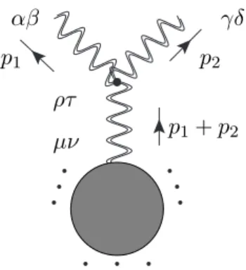
Two gauge bosons of opposite helicities can fuse into a single operator in the same way as in the case of identical helicities. The form of the corresponding OPE terms [15] follows from the collinear limit of gauge interactions. In the case of opposite helicities, however, gravitational interactions allow the fusion of two gauge bosons into a graviton operator [18]. As explained in Appendix A, EYM amplitudes involving gravitational couplings do not blow up in the collinear limit but contain another type of singularity. It is due to a phase ambiguity reflecting an azimuthal asymmetry. In Appendix A, we show that when z

1

→ z

2

,

M (1

⁺

, 2

⁻

, 3, . . . , N ) = 1

¯ z

₁₂

ω

₁

ω

₂

ω

_P

M (P

⁺

, 3, . . . , N ) + 1 z

₁₂

ω

₂

ω

₁

ω

_P

M (P

⁻

, 3, . . . , N )

− z

₁₂

¯ z

₁₂

ω

²₁

ω

_P²

M (P

⁺⁺

, 3, . . . , N ) − z ¯

₁₂

z

₁₂

ω

²₂

ω

_P²

M (P

⁻⁻

, 3, . . . , N )

+ regular . (2.10)

Here, P is the combined momentum of the collinear pair:

P = p

₁

+ p

₂

≡ ω

_P

q

_P

, (2.11)

with

ω

_P

= ω

₁

+ ω

₂

q

_P

= q

₁

= q

₂

(z

_P

= z

₁

= z

₂

, z ¯

_P

= ¯ z

₁

= ¯ z

₂

) , (2.12) and

z

_ij

≡ z

_i

− z

_j

, z ¯

_ij

= ¯ z

_i

− z ¯

_j

. (2.13) In Eq.(2.10), the last two terms, which originate from gravitational couplings,

³

contain the phase factors z

₁₂

/¯ z

₁₂

and z ¯

₁₂

/z

₁₂

depending on the direction from which z

₁

approaches z

₂

or equivalently, on the azimuthal angle of the plane spanned by the collinear pair about the axis of the combined momentum P . The “regular” part does not contain neither z

₁₂

nor

¯

z

₁₂

in denominators and is well-defined, finite in the z

₁

= z

₂

limit. By following the same steps as in Ref.[15], we obtain

O

^a∆1,−

(z, z) ¯ O

∆^b2,+

(w, w) = ¯ C

_(−,+)−

(∆

₁

, ∆

₂

)

z − w

X

c

f

^abc

O

(∆^c 1+∆2−1),−

(w, w) ¯ (2.14) + C

₍₋₊₎₊

(∆

₁

, ∆

₂

)

¯ z − w ¯

X

c

f

^abc

O

(∆^c 1+∆2−1),+

(w, w) ¯ + C

₍₋₊₎₋₋

(∆

₁

, ∆

₂

) z ¯ − w ¯

z − w δ

^ab

O

(∆1+∆2),−2

(w, w) ¯ + C

₍₋₊₎₊₊

(∆

₁

, ∆

₂

) z − w

¯

z − w ¯ δ

^ab

O

(∆1+∆2),+2

(w, w) + ¯ regular , with

C

_(−,+)−

(∆

₁

, ∆

₂

) = ∆

1

− 1

∆

₂

(∆

₁

+ ∆

₂

− 2) , (2.15)

C

_(−,+)+

(∆

₁

, ∆

₂

) = ∆

₂

− 1

∆

1

(∆

1

+ ∆

2

− 2) , (2.16)

C

₍₋₊₎₋₋

(∆

₁

, ∆

₂

) = − 2(∆

₁

− 1)(∆

₁

+ 1)(∆

₂

− 1)

∆

2

(∆

1

+ ∆

2

)(∆

1

+ ∆

2

− 1) , (2.17) C

₍₋₊₎₊₊

(∆

1

, ∆

2

) = − 2(∆

2

− 1)(∆

2

+ 1)(∆

1

− 1)

∆

₁

(∆

₁

+ ∆

₂

)(∆

₁

+ ∆

₂

− 1) . (2.18) The above result agrees with Refs.[15, 18].

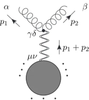
The OPEs involving gravitons can be extracted in a similar way. For two gravitons with identical helicities, we show in Appendix A that

M (1

⁺⁺

, 2

⁺⁺

, 3, . . . , N ) = ω

_P²

ω

₁

ω

₂

¯ z

₁₂

z

₁₂

M (P

⁺⁺

, 3, . . . , N) + regular . (2.19) As a result,

O

∆1,+2

(z, z) ¯ O

∆2,+2

(w, w) = ¯ C

_(+2,+2)+2

z ¯ − w ¯

z − w O

(∆1+∆2),+2

(w, w) + ¯ regular, (2.20)

3In our units, the gravitational and gauge coupling constantsκ= 2andgYM= 1, respectively.

with

C

_(+2,+2)+2

= (∆

₁

+ ∆

₂

− 2)(∆

₁

+ ∆

₂

+ 1)

2(∆

1

+ 1)(∆

2

+ 1) . (2.21) and a similar expression with the conjugated phase factor and the same OPE coefficient for two − 2 helicities.

The collinear limit of two gravitons with opposite helicities is also derived in Appendix A. It reads:

M (1

⁻⁻

, 2

⁺⁺

, 3, . . . , N ) = ω

³₁

ω

_P²

ω

₂

¯ z

₁₂

z

₁₂

M (P

⁻⁻

, 3, . . . , N ) + ω

³₂

ω

²_P

ω

₁

z

₁₂

¯

z

₁₂

M (P

⁺⁺

, 3, . . . , N ) + regular. (2.22) The corresponding OPE is

O

^∆1,−2

(z, z) ¯ O

^∆2,+2

(w, w) = ¯ C

_{(−2,+2)−2}

z ¯ − w ¯

z − w O

(∆1+∆2),−2

(w, w) ¯ (2.23) + C

_(−2,+2)+2

z − w

¯

z − w ¯ O

(∆1+∆2),+2

(w, w) + ¯ regular, with

C

_{(−2,+2)−2}

= 1 2

∆

₁

(∆

₁

− 1)(∆

₁

+ 2)

(∆

₂

+ 1)(∆

₁

+ ∆

₂

− 1)(∆

₁

+ ∆

₂

) , (2.24) C

_(−2,+2)+2

= 1

2

∆

₂

(∆

₂

− 1)(∆

₂

+ 2)

(∆

₁

+ 1)(∆

₁

+ ∆

₂

− 1)(∆

₁

+ ∆

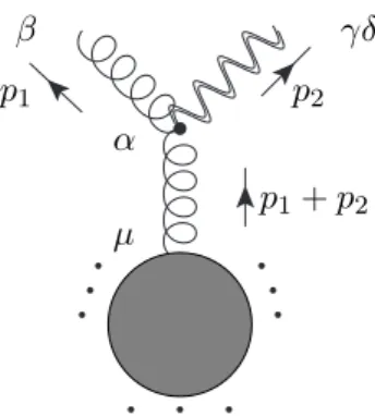
₂

) . (2.25) We close this section by listing the OPEs of gauge bosons with gravitons. They follow from the collinear limits of EYM amplitudes discussed in Appendix A:

M (1

⁺⁺

, 2

⁺

, 3, . . . , N) = ω

_P

ω

₁

¯ z

₁₂

z

₁₂

M (P

⁺

, 3, . . . , N) + regular, (2.26) M (1

⁻⁻

, 2

⁺

, 3, . . . , N) = ω

₂²

ω

_P

ω

₁

z

₁₂

¯

z

₁₂

M (P

⁺

, 3, . . . , N ) + regular, (2.27) which lead to

O

∆1,+

(z, z) ¯ O

∆2,+2

(w, w) = ¯ C

_(+,+2)+

z ¯ − w ¯

z − w O

(∆1+∆2),+

(w, w) + ¯ regular, (2.28) O

∆1,+

(z, z) ¯ O

∆2,−2

(w, w) = ¯ C

_(+,−2),+

z − w

¯

z − w ¯ O

(∆1+∆2),+

(w, w) + ¯ regular, (2.29) with

C

_(+,+2)+

= 1 2

(∆

₁

− 1)(∆

₁

+ ∆

₂

)

∆

₁

(∆

₂

+ 1) , (2.30)

C

_(+,−2)+

= 1 2

(∆

₁

− 1)(∆

₁

+ 1)

(∆

₂

+ 1)(∆

₁

+ ∆

₂

− 1) . (2.31)

The OPEs of operators with + and − interchanged have the phase factors (z − w)/(¯ z − w) ¯

conjugated and the same coefficients.

3 OPEs of superrotations and supertranslations with spin 1 and spin 2 operators

In this section, we discuss the OPEs of superrotations generated by the energy momentum tensor T and of supertranslations generated by the operator P , with the operators associated to gauge bosons and gravitons. We know what to expect from the OPE of T with primary fields. In Ref.[13], we showed that the operators O

∆,±^a

representing gauge bosons are indeed such primary fields. To that end, we used the energy-momentum tensor defined in [16, 17]

as the shadow [25] of dimension ∆ = 0 graviton operator O

0,−2

: T (z) ≡ O e

∆→0,−2

(z, z) = ¯ 3!

2π Z

d

²

z

^′

1

(z

^′

− z)

⁴

O

0,−2

(z

^′

, z ¯

^′

) (3.1) and took the collinear limit of the shadow with gauge bosons as in Eq.(2.27). The limit of

∆ → 0 was taken at the end. Actually, as we will see in this section, there is a fast way of deriving and generalizing the results of Ref.[13]. We will first take the ∆ → 0 limit and then take the shadow transform in order to extract the OPEs. We will proceed in the same way in the case of P :

P (z, z) ¯ ≡ ∂

_z¯

O

∆→1,+2

, (3.2)

by taking the ∆ → 1 limit first.

3.1 Superrotations

We start by inserting T(z) into the correlator (2.6):

D T (z) Y

N n=1

O

∆ⁿ,ℓⁿ

(z

_n

, z ¯

_n

) E

= lim

∆0→0

Y

^N

n=0

c

_n

(∆

_n

) 3!

2π Z

d

²

z

₀

1 (z

₀

− z)

⁴

× A

ℓ0=−2,ℓ1...ℓ^N

(∆

_n

, z

_n

, z ¯

_n

) (3.3) where we used the definition (3.1) and

A

ℓ0=−2,ℓ1...ℓN

(∆

_n

, z

_n

, z ¯

_n

) ≡ A

−2

(∆

₀

, ∆

₁

, . . . , ∆

_N

) (3.4)

= Y

^N

n=0

Z

dω

n

ω

^∆_nⁿ⁻¹

δ

⁽⁴⁾

X

N n=0

ǫ

n

ω

n

q

n

M

ℓ0=−2,ℓ1...ℓ^N

(ω

n

, z

n

, z ¯

n

) , which is the Mellin-transformed amplitude with a “soft” graviton. Its ∆

₀

→ 0 limit has been studied in Refs.[21–23], with the following result:

A

−2

(∆

₀

, ∆

₁

, . . . , ∆

_N

) (3.5)

−→ 1

∆

₀

X

N

i=1

(z

₀

− z

_i

) (¯ z

₀

− z ¯

_i

)

(¯ ξ − z ¯

_i

) (¯ ξ − z ¯

₀

)

h (z

₀

− z

_i

)∂

_zi

− 2h

_i

i

A (∆

₁

, . . . , ∆

_N

)

where A on the r.h.s. is the Mellin transform of the amplitude without the graviton. Here,

h

_i

is the chiral weight of the ith operator and ξ is an arbitrary reference point on CS

²

reflecting the gauge choice for the graviton. In this case, it is convenient to set ξ → ∞ . The shadow transform can be performed by writing

1

(z

₀

− z)

⁴

= − 1

3! ∂

_z³₀

1 z

₀

− z

(3.6)

and integrating by parts three times. After repeatedly using the identity

∂

_z0

1

¯ z

₀

− z ¯

_i

= 2πδ

⁽²⁾

(z

₀

− z

_i

) , (3.7)

we obtain

D T (z) Y

N n=1

O

∆ⁿ,ℓⁿ

(z

_n

, z ¯

_n

) E

= lim

∆0→0

c

₀

(∆

₀

)

∆

₀

(3.8)

× X

N

i=1

h

− 2h

i

(z − z

_i

)

²

− 2 z − z

_i

∂

zi

iD Y

^N

n=1

O

∆ⁿ,ℓⁿ

(z

n

, z ¯

n

) E . Note that

∆

lim

0→0

c

₀

(∆

₀

)

∆

₀

= lim

∆0→0

f (∆

₀

)

∆

₀

= − 1

2 , (3.9)

see Eq.(2.5). As a result, we obtain T (z) O

∆,ℓ

(w, w) = ¯ h

(z − w)

²

O

∆,ℓ

(w, w) + ¯ 1

z − w ∂

_w

O

∆,ℓ

(w, w) + ¯ regular . (3.10) Following the same route for the antiholomorphic T ¯ (¯ z), one obtains

T ¯ (¯ z) O

∆,ℓ

(w, w) = ¯ ¯ h

(¯ z − w) ¯

²

O

∆,ℓ

(w, w) + ¯ 1

¯

z − w ¯ ∂

_w¯

O

∆,ℓ

(w, w) + ¯ regular . (3.11) The OPEs (3.10) and (3.11), which are valid for both spin 1 and spin 2 particles, prove that the respective CCFT operators are primary fields.

3.2 Supertranslations

We start by inserting P(z

0

) into the correlator (2.6):

D P(z

₀

) Y

N n=1

O

∆ⁿ,ℓⁿ

(z

_n

, z ¯

_n

) E

= lim

∆0→1

Y

^N

n=0

c

_n

(∆

_n

)

∂

_z¯0

A

ℓ=+2,ℓ1...ℓN

(∆

_n

, z

_n

, z ¯

_n

) (3.12) where we used the definition (3.2). In this case, the relevant ∆

₀

→ 1 soft limit is [21–23]:

A

+2

(∆

₀

, ∆

₁

, . . . , ∆

_N

) (3.13)

−→ 1

∆

₀

− 1 X

N

i=1

(¯ z

₀

− z ¯

_i

) (z

₀

− z

_i

)

(ξ − z

_i

)

²

(ξ − z

₀

)

²

A (∆

₁

, . . . , ∆

_i

+ 1, . . . , ∆

_N

)

Here again, as in Eq.(3.5), we can set ξ → ∞ . From Eqs.(3.12) and (3.13) it follows that D P(z

0

)

Y

N n=1

O

∆ⁿ,ℓⁿ

(z

n

, ¯ z

n

) E

= lim

∆0→1

c

0

(∆

0

)

∆

₀

− 1 X

^N

i=1

c

i

(∆

i

) c

_i

(∆

_i

+ 1)

1

z

₀

− z

_i

(3.14)

× D h

ⁱ⁻¹

Y

m=1

O

∆m,ℓm

(z

_m

, z ¯

_m

) i

O

∆i+1,ℓi

(z

_i

, z ¯

_i

) h Y

^N

n=i+1

O

∆n,ℓn

(z

_n

, z ¯

_n

) i E . Note that

∆

lim

0→1

c

₀

(∆

₀

)

∆

₀

− 1

= lim

∆0→1

f (∆

₀

)

∆

₀

− 1 = 1

4 (3.15)

and

c

_i

(∆

_i

) c

_i

(∆

_i

+ 1) =

 



g(∆i)

g(∆i+1)

=

^{(∆i−1)(∆}_∆ ⁱ⁺¹⁾

i

for ℓ

_i

= ± 1,

f(∆ⁱ)

f(∆ⁱ+1)

=

^{(∆i−1)(∆}_∆i+1ⁱ⁺²⁾

for ℓ

i

= ± 2, (3.16) As a result, we obtain

P(z) O

∆,ℓ

(w, w) = ¯ (∆ − 1)(∆ + 1) 4∆

1

z − w O

∆+1,ℓ

(w, w) + ¯ regular (ℓ = ± 1), (3.17) P (z) O

∆,ℓ

(w, w) = ¯ (∆ − 1)(∆ + 2)

4(∆ + 1)

1

z − w O

∆+1,ℓ

(w, w) + ¯ regular (ℓ = ± 2), (3.18) and similar expressions for P ¯ (¯ z), with complex conjugate poles.

⁴

Note the presence of (∆ − 1) factors in the above OPE coefficients. They imply that the products P(z)J

^a

(w), P (z) ¯ J

^a

( ¯ w), P (z)P(w) and P (z) ¯ P ( ¯ w) are regular.

P(z) is not a holomorphic current: it is a dimension 2 descendant of a primary field, with SL(2, C ) weights (3/2,1/2). Nevertheless, the r.h.s. of Eq.(3.14) implies the same Ward identity as translational symmetry of scattering amplitudes discussed in Refs.[26] and [27].

In fact, P contains the P

₀

+ P

₃

component of the momentum operator which generates translations along the light-cone directions. The remaining components can be obtained by superrotations of P . This will be discussed in Section 5.

4 OPEs of BMS generators 4.1 T T

The product of energy-momentum tensors involves two shadow transforms. Let us define A ee (w, z, z

₂

, . . . ) =

Z

d

²

z

₀

1 (z

₀

− w)

⁴

Z

d

²

z

₁

1

(z

₁

− z)

⁴

A

ℓ0=−2,ℓ1=−2,ℓ2...ℓN

. (4.1) Then

D T (w)T (z) Y

N n=2

O

∆ⁿ,ℓⁿ

(z

_n

, z ¯

_n

) E

= 3!

2π

2

∆

lim

1→0

lim

∆0→0

Y

N n=0

c

_n

(∆

_n

)

A ee (w, z, z

₂

, . . . ) . (4.2)

4The same result can be obtained from Eqs.(2.20), (2.23) and (2.28), derived in the previous section by considering the collinear instead of soft limits, by taking the limit of∆2→1.

We take the limit ∆

0

→ 0 first, as in Eq.(3.5):

A

ℓ0=−2,ℓ1=−2,ℓ1...ℓ^N

−→ 1

∆

₀

X

N i=1

(z

₀

− z

_i

) (¯ z

₀

− z ¯

_i

)

(¯ ξ − z ¯

_i

) (¯ ξ − z ¯

0

)

h (z

₀

− z

_i

)∂

_zi

− 2h

_i

i

A

ℓ1=−2,ℓ2...ℓ^N

, (4.3) which leads to

A ee (w, z, z

₂

, . . . ) ∼

Z d

²

z

0

(z

₀

− w)

⁴

Z d

²

z

1

(z

₁

− z)

⁴

(z

0

− z

1

) (¯ z

₀

− z ¯

₁

)

(¯ ξ − z ¯

1

) (¯ ξ − z ¯

₀

)

h (z

₀

− z

₁

)∂

_z1

− 2h

⁻₁

i

A

ℓ1=−2,ℓ2...ℓ^N

+

Z d

²

z

0

(z

₀

− w)

⁴

X

N

i=2

(z

0

− z

i

) (¯ z

₀

− z ¯

_i

)

(¯ ξ − ¯ z

i

) (¯ ξ − z ¯

₀

) h

(z

0

− z

i

)∂

zi

− 2h

i

i !

A e (z, z

2

, . . . ) , (4.4) where h

⁻₁

= − 1 because ℓ

₁

= − 2, ∆

₁

= 0 and

A e (z, z

₂

, . . . ) =

Z d

²

z

₁

(z

₁

− z)

⁴

A

ℓ1=−2,ℓ2...ℓN

. (4.5) In Eq.(4.4), the integrals over z

₀

can be performed by using the conformal integrals of Ref.[28], see Appendix B. With the reference point ξ → ∞ , the result is

∆

lim

0→0

3!

2π c

₀

(∆

₀

) A ee (w, z, z

₂

, . . . ) =

Z d

²

z

₁

(z − z

₁

)

⁴

h

⁻₁

(w − z

₁

)

²

+ 1 w − z

₁

∂

_z1

A

ℓ1=−2,ℓ2...ℓN

+ X

N

i=2

h

i

(w − z

_i

)

²

+ 1 w − z

_i

∂

zi

A e (z, z

2

, . . . ) , (4.6) The same result can be obtained by a direct application of Ward identity (3.8).

It is clear from Eq.(4.6) that the second term (involving the sum over i ≥ 2) is non- singular in the limit of w → z, therefore only the first term needs to be included in the derivation of OPE:

h T (w)T (z) Y

N n=2

O (z

_n

, z ¯

_n

) i = (4.7)

= lim

∆1→0

3!

2π

Z d

²

z

₁

(z − z

₁

)

⁴

1

w − z

₁

∂

_z1

− 1 (w − z

₁

)

²

G

⁻

(z

₁

, . . . ) , where

G

⁻

(z

₁

, . . . ) = hO

∆1,−2

(z

₁

, z ¯

₁

) Y

N n=2

O (z

_n

, z ¯

_n

) i . In order to simplify notation, we introduce the following variables:

Z = z − z

1

, W = w − z

1

. (4.8)

We anticipate a single pole term of the following form:

1 w − z h ∂T

Y

N n=2

O (z

n

, z ¯

n

) i = lim

∆1→0

3!

2π 1 w − z ∂

z

Z d

²

z

1

Z

⁴

G

⁻

(z

1

, . . . )

= lim

∆1→0

3!

2π

− 1 w − z

Z d

²

z

₁

∂

_z1

1 Z

⁴

G

⁻

(z

₁

, . . . )

= lim

∆1→0

3!

2π 1 w − z

Z d

²

z

1

Z

⁴

∂

z1

G

⁻

(z

1

, . . . ) , (4.9)

where in the last step we used integration by parts. Indeed, we can rewrite the r.h.s. of (4.7) as

∆

lim

1→0

3!

2π Z

d

²

z

₁

− 1

Z

⁴

W

²

+ 1 Z

⁴

W ∂

_z1

G

⁻

(z

₁

, . . . ) =

= lim

∆1→0

3!

2π

− 1 Z

⁴

W

²

+

1

Z

⁴

− 1 Z

³

W

1 w − z ∂

_z1

G

⁻

(z

₁

, . . . ) = (4.10)

= − lim

∆1→0

3!

2π 1

Z

⁴

W

²

+ 1 w − z

1 Z

³

W ∂

_z1

G

⁻

(z

₁

, . . . ) + 1

w − z h ∂T (z) · · · i . In the last line, the first term can be written as

∆

lim

1→0

3!

2π 2

(w − z)

²

Z d

²

z

₁

Z

⁴

G

⁻

(z

₁

, . . . ) − 2 w − z

Z d

²

z

₁

1 w − z

1

Z

³

W − 1 Z

³

W

²

G

⁻

(z

₁

, . . . )

= 2

(w − z)

²

h T (z) · · · i − lim

∆1→0

3!

2π 2 (w − z)

²

Z

d

²

z

₁

1

Z

²

W

²

G

⁻

(z

₁

, . . . ) . (4.11) After combining Eqs.(4.10) and (4.11), we obtain:

h T (w)T (z) Y

N n=2

O (z

_n

, z ¯

_n

) i = 2

(w − z)

²

h T (z) Y

N n=2

O (z

_n

, z ¯

_n

) i + 1

w − z h ∂T (z) Y

N n=2

O (z

_n

, z ¯

_n

) i

− lim

∆1→0

3!

2π 2 (w − z)

²

Z

d

²

z

1

1

Z

²

W

²

G

⁻

(z

1

, . . . ) . (4.12) The final step is to show that the last term vanishes due to global conformal invariance. To that end, we take the soft limit ∆

₁

→ 0:

G

⁻

(z

₁

, . . . ) → c(∆

₁

)

∆

₁

X

N i=2

z

₁

− z

_i

¯ z

₁

− ¯ z

_i

¯ σ − z ¯

_i

¯

σ − z ¯

₁

[(z

₁

− z

_i

)∂

_i

− 2h

_i

] h Y

N n=2

O (z

_n

, z ¯

_n

) i . (4.13) After choosing the reference point σ = z, the derivative terms become

Z d

²

z

₁

Z

²

W

²

(z

₁

− z

_i

)

²

(¯ z

₁

− z ¯

_i

)(¯ z

₁

− z) ¯ (¯ z

_i

− z)∂ ¯

_i

h Y

N n=2

O (z

_n

, z ¯

_n

) i = (4.14)

= Γ(0)

− 1

(z − w)

³

(z

i

− w)

²

∂

i

+ 1

(z − w)

²

(z

i

− w)∂

i

h

Y

N n=2

O (z

n

, z ¯

n

) i , where we used conformal integrals of Ref.[28], see Appendix B, in particular Eq.(B.3).

⁵

The remaining terms can be written as

− 2h

_i

∂

_w

Z d

²

z

₁

Z

²

W

z

₁

− z

_i

(¯ z

₁

− z ¯

_i

)(¯ z

₁

− z) ¯ (¯ z

_i

− z) ¯ h Y

N n=2

O (z

_n

, z ¯

_n

) i (4.15)

= 2h

_i

Γ(0)

1

(z − w)

²

+ 2 w − z

_i

(z − w)

³

h

Y

N n=2

O (z

_n

, z ¯

_n

) i . (4.16)

5The integrals are divergent as it is obvious from the presence of theΓ(0)prefactor. We can regularize the divergence by taking the soft limit on the shadow transform at the end. In other words use

Z d²z1

(z−z1)^4+iλ(¯z−z¯1)^iλ and takeλ→0at the end. Our results will be the same

In this way, the last term of Eq.(4.12) becomes 2Γ(0)

"

− 1 (z − w)

³

X

N i=2

[(z

_i

− w)

²

∂

_i

+ 2h

_i

(z

_i

− w)] h Y

N n=2

O (z

_n

, z ¯

_n

) i

#

(4.17)

+ 2Γ(0)

"

1 (z − w)

²

X

N i=2

[(z

_i

− w)∂

_i

+ h

_i

] h Y

N n=2

O (z

_n

, z ¯

_n

) i

#

= 0 , (4.18)

with both terms vanishing separately as a consequence of global conformal (Lorentz) in- variance [26]:

X

N i=2

∂

_i

h Y

N n=2

O (z

_n

, z ¯

_n

) i = X

N i=2

(z

_i

∂

_i

+ h

_i

) h Y

N n=2

O (z

_n

, z ¯

_n

) i =

= X

N i=2

z

_i²

∂

_i

+ 2z

_i

h

_i

h

Y

N n=2

O (z

_n

, z ¯

_n

) i = 0 . The final result is the expected T (w)T(z) OPE:

T (w)T (z) = 2T (z)

(w − z)

²

+ ∂

_z

T (z)

w − z + regular . (4.19)

4.2 T T

By repeating the steps leading to Eq.(4.7), we obtain h T (w)T (z)

Y

N n=2

O (z

_n

, z ¯

_n

) i = (4.20)

= lim

∆1→0

3!

2π

Z d

²

z

₁

(¯ z − ¯ z

₁

)

⁴

1

w − z

₁

∂

_z1

+ 1 (w − z

₁

)

²

G

⁺

(z

₁

, . . . ) , where

G

⁺

(z

1

, . . . ) = hO

⁺∆1,+2

(z

1

, z ¯

1

) Y

N n=2

O (z

n

, z ¯

n

) i , (4.21) which can be simplified to

h T (w)T (z) Y

N n=2

O (z

_n

, z ¯

_n

) i = − lim

∆1→0

3!

2π

Z d

²

z

₁

w − z

₁

G

⁺

(z

₁

, . . . )∂

_z1

(¯ z − z ¯

₁

)

⁻⁴

. After using

∂

_z1

(¯ z − z ¯

₁

)

⁻⁴

= 1

3! ∂

_z1

∂ ¯

_z³_¯1

1

¯

z − z ¯

₁

= 2π

3! ∂ ¯

_z³_¯1

δ

⁽²⁾

(z − z

₁

) , (4.22) we obtain

h T (w)T (z) Y

N n=2

O (z

_n

, z ¯

_n

) i = − lim

∆1→0

Z d

²

z

₁

w − z

₁

G

⁺

(z

₁

, . . . ) ¯ ∂

_¯z³₁

δ

⁽²⁾

(z − z

₁

)

= lim

∆1→0

∂ ¯

_¯z³

G

⁺

(z, . . . ) w − z

. (4.23)

Note that in the soft limit

∆

lim

1→0

G

⁺

(z, . . . ) = − 1 2

X

N i=2

¯ z − z ¯

_i

z − z

_i

σ − z

_i

σ − z

(¯ z − z ¯

_i

)∂

_i

− 2h

_i

h

Y

N n=2

O (z

_n

, z ¯

_n

) i , (4.24) therefore the derivative ∂ ¯

_z³_¯

acting on the r.h.s. of Eq.(4.23) gives zero modulo delta-function terms localized at z = w and z = z

_n

. These terms do not affect the Virasoro algebra following from Eq.(4.19). We conclude that up to such delta functions,

T (w)T(z) = regular . (4.25)

4.3 T P and T P

Recall (3.2) that the supertranslation current is defined as

P (z) = ∂

_z¯

O

1,+2

(z, z) ¯ . (4.26) The graviton primary field operator O

1,+2

has chiral weights (

³₂

, −

¹₂

). We start from

h T (w)P(z) Y

N n=2

O (z

_n

, z ¯

_n

) i = lim

∆0→0

lim

∆1→1

Y

^N

n=0

c(∆

_n

) 3!

2π

× Z

d

²

z

₀

1

(z

0

− w)

⁴

∂

_¯z

A

ℓ0=−2,ℓ1=+2,ℓ2...ℓ^N

. (4.27) In the ∆

₀

→ 0 limit, c.f. Eq.(4.3) with ℓ

₁

= +2 and the reference point ξ → ∞ ,

∂

_z¯

lim

∆0→0

Y

^N

n=0

c(∆

_n

)

A

ℓ0=−2,ℓ1=+2,ℓ2...ℓN

= − 1

2 ∂

z¯

(z

0

− z)

(¯ z

₀

− z) ¯ [(z

0

− z)∂

z

− 2h

1

] G

⁺

(z, z

2

, . . . )

− 1 2 ∂

_z¯

X

N i=2

(z

₀

− z

_i

)

(¯ z

₀

− z ¯

_i

) [(z

₀

− z

_i

)∂

_zi

− 2h

_i

] G

⁺

(z, z

₂

, . . . ) , (4.28) with G

⁺

defined in Eq.(4.21) and h

1

=

³₂

. As in previous cases, the sum over i ≥ 2 is non-singular at z = w, therefore we are left with

∂

_z¯

lim

∆0→0

Y

^N

n=0

c(∆

_n

)

A

ℓ0=−2,ℓ1=+2,ℓ2...ℓN

(4.29)

= 1 2

h 3 z

₀

− z

(¯ z

₀

− z) ¯

²

− (z

₀

− z)

²

(¯ z

₀

− z) ¯

²

∂

_z

+ 3 z

₀

− z

¯

z

₀

− z ¯ ∂

_¯z

− (z

₀

− z)

²

(¯ z

₀

− z) ¯ ∂

_z

∂

_z¯

i

G

⁺

(z, z

₂

, . . . ) + . . . Upon inserting the above expression into the shadow integral of Eq.(4.34), the first two terms give rise to delta-function singularities at z = w, but vanish for z 6 = w. In particular,

3

Z d

²

z

0

(z

₀

− w)

⁴

z

0

− z

(¯ z

₀

− z) ¯

²

= ∂

_w

Z d

²

z

0

(z

₀

− w)

³

z

0

− z

(¯ z

₀

− z) ¯

²

∼ ∂

_w

δ

⁽²⁾

(z − w) . (4.30)