RichardMommertz submittedby Master’sthesis MappingbedfastandfloatingthermokarstlakeiceanddetermininglakedepthusingSentinel1SyntheticApertureRadarRemoteSensingonthewestshoreofHudsonBay,CanadaandPrudhoeBay,Alaska

(1)

University of Potsdam

Institute for Earth- and Environmental Science MSc Geoecology

Mapping bedfast and floating thermokarst lake ice and determining lake depth using Sentinel 1 Synthetic Aperture Radar Remote Sensing on the

west shore of Hudson Bay, Canada and Prudhoe Bay, Alaska

Master’s thesis

submitted by Richard Mommertz

Registration number: 784651

Address: Thaerstr. 15, 14469 Potsdam Email: richard.mommertz@uni-potsdam.de

Date: 18 June 2019

(2)

Supervisors Prof. Dr. Bodo Bookhagen Universität Potsdam

Institut für Geowissenschaften Karl-Liebknecht-Str. 24–25 14476 Potsdam-Golm Dr. Moritz Langer Alfred Wegener Institute Telegrafenberg A45 14473 Potsdam

(3)

Abstract

Thermokarst lakes are an abundant feature in Arctic permafrost regions and cover up to 40 percent of the land area. During winter shallow lakes freeze to the bed (bedfast ice) while lakes which are deeper than the maximum ice thickness up to 2 m preserve perennial liquid water below the ice (floating ice). The different lake ice regimes have an impact on the energy distribution to the surrounding permafrost, available aquatic habitat and geomorphological processes.

Completely frozen lakes contribute less energy and gas fluxes to the landscape and atmosphere while floating ice conditions support the development of a talik, a continu- ously unfrozen layer, as the remaining liquid water provides energy to the surrounding permafrost. This has an impact on permafrost thawing and geomorphological development as taliks can favour subsurface lake drainage, permafrost degradation and lateral lake erosion. Bedfast or floating ice conditions are dependant on the maximum ice thickness. Ice growth is determined by winter temperatures and snow conditions as a thicker snow cover provides insulation and reduce ice growth.

In this study Sentinel 1 synthetic aperture radar (SAR) data for four winters from 2015 to 2018 was used to investigate thermokarst lakes and compare lake ice regimes in two study areas with permafrost conditions. One is in the area of Prudhoe Bay, North Slope Borough, Alaska and the other on the west shore of Hudson Bay near Churchill, Manitoba, Canada. Synthetic aperture radar remote sensing allows to distinguish between bedfast and floating ice due to different backscatter intensities. While bedfast ice absorbs the radar signal and appears dark on the radar image, floating ice shows a strong reflectance and appears bright. This is due to differences in the dielectric contrast between ice and sediment (lake bed) and ice and liquid water, respectively.

Additionally the maximum ice thickness was approximated by calculating ice growth based on freezing degree days from MODIS land surface temperature data. With the resulting ice growth curve the maximum water depth of lakes which freeze completely to the ground was determined through the date when they became bedfast.

Bedfast lake ice percentages decreased over the study period in Prudhoe Bay while they varied widely in Churchill. The average proportions were similar for both study areas with 68 % in Prudhoe Bay and 62 % in Churchill. The lakes in Prudhoe Bay showed a trend towards floating ice regimes which was not detectable in Churchill. Relationships between winter temperatures and the amount of bedfast ice were not linear and indicate the presence of tipping points. Maximum ice thickness was estimated to be 160 cm in Prudhoe Bay which seems valid, while the similar ice thickness in Churchill is most likely overestimated by the used method.

Future work in permafrost regions and the establishment of long term observations should help to understand trends more reliable and detect relationships between climate and resulting landscape responses.

(4)

Zusammenfassung

Thermokarst Seen sind ein wichtiges Merkmal in arktischen Permafrostregionen und bedecken bis zu 40 Prozent der Landfläche. Während des Winters frieren flache Seen bis zum Grund (bedfast ice), während Seen deren Tiefe die maximale Eisdicke von bis zu 2 m übersteigt, dauerhaft flüssiges Wasser unter dem Eis behalten (floating ice).

Diese unterschiedlichen Seeeisregime haben einen Einfluss auf die Energieabgabe zu dem umgebenen Permafrost, den verfügbaren aquatischen Habitaten und geomorphol- ogischen Prozessen.

Vollständig gefrorene Seen bringen weniger Energie- und Gasflüsse in die Landschaft und Atmosphäre ein, wohingegen schwimmende Eisbedingungen die Entwicklung einer Talik, einer kontinuierlich ungefrorenen Schicht, begünstigen, da das flüssige Wasser Wärmeenergie an den umgebenen Permafrost abgibt. Das hat einen Einfluss auf das Tauen von Permafrost sowie auf geomorphologische Prozesse, da Taliks Seedrainagen, Permafrostdegradation und laterale Erosion begünstigen können. Die maximale Eis- dicke entscheidet über vollständig gefrorene oder schwimmende Eisbedingungen. Die Eisdicke hängt von Wintertemperaturen und Schneefall ab, da eine größere Schneedecke isolierende Wirkung hat und das Eiswachstum verlangsamt.

In dieser Arbeit wurden Sentinel 1 Synthetic Aperture Radar (SAR) Daten von vier Wintern in den Jahren 2015 bis 2018 zur Untersuchung von Thermokarstseen genutzt.

Es wurden zwei Untersuchungsgebiete mit Permafrostbedingungen ausgesucht, im Ge- biet von Prudhoe Bay, Alaska und an der Westküste der Hudson Bay in der Nähe der Stadt Churchill, Manitoba, Kanada. Synthetic Aperture Radar Fernerkundung ermöglicht die Unterscheidung zwischen vollständig gefrorenen Seen und schwimmen- dem Eis aufgrund der unterschiedlichen Rückstreuung. Bis zum Grund gefrorenes Wasser absorbiert das Radarsignal während schwimmendes Eis es reflektiert. Das liegt an dem unterschiedlichen dielektrischen Kontrast zwischen Eis und Sedimenten beziehungsweise Eis und flüssigem Wasser. Auf dem Radarbild zeigt sich das durch dunkle und helle Pixel. Zusätzlich wurde die maximale Eisdicke mithilfe von MODIS Oberflächentemperaturen berechnet. Die Eiswachstumskurve wurde dazu genutzt die Wassertiefen von Seen abzuschätzen, die bis zum Grund durchfrieren.

In Prudhoe Bay verringerte sich der Anteil an bedfast Eis im Beobachtungszeitraum während er in Churchill stark schwankte. In beiden Untersuchungsgebieten waren die durchschnittlichen Anteile sehr ähnlich (Prudhoe Bay 68 % und Churchill 62 %).

Es wurde ein Trend hin zu floating Eisregimen der Seen in Prudhoe Bay festgestellt.

Dieser ist nicht sichtbar in Churchill. Der Vergleich von Wintertemperaturen und den vorherrschenden Eisregimen zeigte keinen linearen Zusammenhang. Das deutet auf die Existenz von Tipping-Points hin. Die maximale Eisdicke in Prudhoe Bay wurde auf 160 cm geschätzt. Gemesse Werte zeigen eine ähnliche Größenordnung. Die Eisdicke

(5)

in Churchill hat einen ähnlichen Wert, der allerdings mit großer Sicherheit von der genutzten Methode überschätzt wurde.

Zukünftige Untersuchungen von Permafrostgebieten und die Schaffung von langfristi- gen Beobachtungsreihen können zu einem besseren Verständnis von möglichen Trends und Zusammenhängen führen.

(6)

Contents

List of Figures

1 Schematic of permafrost components . . . 3

2 Distribution of permafrost in the Arctic . . . 4

3 Global lake area distribution in comparison to latitude and permafrost zones . . . 5

4 Illustration of radar scattering . . . 7

5 Study area Prudhoe Bay . . . 9

6 Climographs of Prudhoe Bay and Churchill . . . 10

7 Study area Churchill . . . 12

8 Refined Lee speckle filter . . . 15

9 Bimodal frequency distribution from Sentinel 1 backscatter coefficients 19 10 Bedfast and floating ice pixels in April 2015, 2017 and 2018 in Prudhoe Bay . . . 20

11 Comparison of bedfast ice pixels, FDDs, ice thickness and early winter temperatures in Prudhoe Bay . . . 23

12 Relationship between bedfast ice percentage and FDDs . . . 24

13 Calculated ice growth curve from 01 September 2017 to 31 May 2018 for Prudhoe Bay . . . 25

14 Distribution of water depth in Prudhoe Bay . . . 26

15 Bedfast and floating ice pixels in April 2015, 2016, 2017 and 2018 in Churchill . . . 28

16 Lake ice classification from 15 March and 30 April 2018 in Churchill . . 29

17 Comparison of bedfast ice pixels, FDDs, ice thickness and early winter temperatures in Churchill . . . 30

18 Calculated ice growth curve from 01 September 2017 to 31 May 2018 for Churchill . . . 31

19 Distribution of water depth in Churchill . . . 32

(8)

List of Tables

1 SAR acquisition dates, modes, polarisation, incidence angle and pixel size 18 2 Percentage of bedfast ice pixels in each year in comparison to the amount

of the corresponding freezing degree days in Prudhoe Bay . . . 21 3 Lake ice regimes in percentage of total number of lakes in Prudhoe Bay 21 4 Percentage of bedfast ice pixels in each year in comparison to the amount

of the corresponding freezing degree days in Churchill . . . 27 5 Lake ice regimes in percentage of total number of lakes in Churchill . . 29

(9)

1 Introduction

Permafrost regions have a great importance as they account for a fourth of the total land area in the northern hemisphere. Arctic environments are sensitive to climatic changes. Increasing temperatures and changing snow conditions lead to a warming of Arctic permafrost of up to 2 °C since the 1970s (Vaughan et al. 2013). The Arctic is found to amplify the global climatic system in both past and recent warming phases (Johannessen et al. 2016). Thus, the observation of changes in the Arctic is of particular

importance.

Permafrost warming causes degradation which develops specific geomorphological land- forms such as thermokarst lakes. Those lakes are an abundant feature in Arctic permafrost regions. They are extensively studied with remote sensing methods for a long time. Remote sensing has the advantage of being a cost efficient technique to investigate surface properties. This applies in particular to the large and remote areas in high latitudes which are difficult to access due to harsh climatic conditions and limited infrastructure (Grosse et al. 2013).

Shallow lakes with depths less than the maximum ice thickness of up to 2 m freeze completely during the winter. Those lakes are called bedfast ice lakes in contrast to floating ice lakes which are deeper than the maximum ice thickness and preserve perennial liquid water. The distinction between bedfast and floating lakes is important as it impacts several factors. Bedfast lakes contribute less energy to the ambient permafrost while water temperatures above freezing can cause further permafrost degradation below floating lakes. Furthermore, floating lakes provide important fish overwintering habitats and access to winter water supply for industrial and public demands (Jorgenson et al. 2010; Jones et al. 2013; Arp et al. 2015).

Radar remote sensing allows to distinguish between bedfast and floating ice due to differences in backscatter intensities. It is used for many decades to analyse Arctic lakes. The wavelength characteristics offer distinctive benefits for high latitudes as the signal is transmitted through fog and clouds and is independent from daylight. The first insights were acquired by the use of airborne data. With increasing availability of satellite data more and larger areas could be investigated over longer time spans.

The application of radar remote sensing includes climatic implications, freshwater and habitat mapping, ice thickness assessment, long term lake ice regime classification and estimation of methane ebullition (Mellor 1982; Kozlenko and Jeffries 2000; Walter et al.

2008; Jones et al. 2013; Surdu et al. 2014; Engram et al. 2018).

The main goals of this study are

• to use Sentinel 1 C-band synthetic aperture radar imaging from ESA to classify bedfast and floating lake ice in consecutive years for the data availability period (2014–2018)

(10)

1 Introduction

• to identify potential changes and dependencies between lake ice regimes and climatic factors

• to estimate lake depths with SAR data and a calculated ice growth curve

(11)

2 State of the art

2.1 Permafrost

Permafrost was first defined by Muller (1947) as permanently frozen ground. Thus, the temperature should be constantly below the freezing point for at least two consecutive years. This definition is nowadays renewed to perennially frozen because permafrost thawing can occur due to rapid changes in climate conditions and is not a constant state. It is characterised by a mean annual ground temperature below the freezing point (Washburn 1973; French 2018) regardless the material. It can be soil or deposits with varying texture, induration and water content as well as bedrock (Muller 1947).

The freezing point of contained water can be below 0 °C due to the increased pressure and dissolved salts (French 2018).

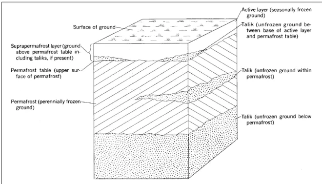
Figure 1 shows different components of permafrost and their positions. The permafrost table is the upper limit of the permafrost. Above the permafrost table is the active layer which is seasonally frozen, this means that it thaws during summer and freezes during winter. Unfrozen zones are called talik whether they are between the active layer and the permafrost table, situated in or below the permafrost.

Figure 1: Schematic of permafrost components: relationship of active layer, permafrost table, permafrost and taliks (Ferrians et al. 1969)

The active layer thickness can vary from a few centimetres in polar regions up to more than one metre in subarctic areas. It is typically reaching the permafrost table in continuous permafrost while it can be detached from the permafrost beneath by a talik (French 2018).

(12)

2.1 Permafrost

In the northern hemisphere the permafrost regions account for approximately 24 % of the total land area (23*10⁶ km²). Cold permafrost with temperatures of -10 °C and less can reach thicknesses of more than 500 m while warm permafrost with subzero temperatures close to 0 °C are only a few decimetres thick (Heginbottom et al. 2012).

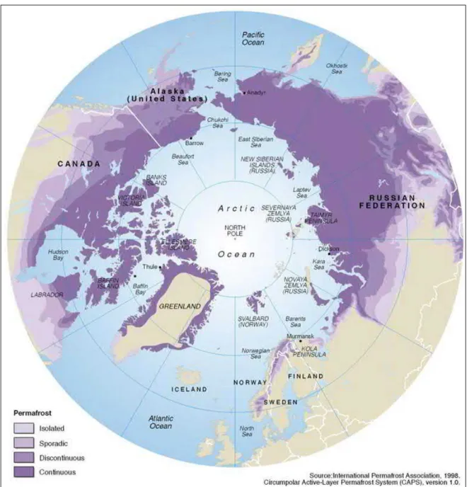
Permafrost can be subdivided into four major zones depending on the area which is occupied by permafrost: continuous (90–100 %), discontinuous (50–90 %), sporadic (10–50 %) and isolated (0–10 %) (figure 2; French 2018).

The zones are based on mean annual air temperature (MAAT). The boundary between the continuous and discontinuous permafrost zones is a MAAT of -8.5 °C which corresponds to a mean annual ground temperature (MAGT) of -5 °C. The southern limit of permafrost is marked by a MAAT of -1 °C (Brown and Péwé 1973).

Figure 2: Distribution of permafrost in the Arctic with delineation into four zones: continuous, discontinuous, sporadic and isolated (Brown et al. 1997)

(13)

2.1 Permafrost

Land forms of ice rich permafrost regions include pingos and polygonal tundra, the typical landform of the Arctic Coastal Plain. Pingos are conical hills which develop preferably in drained basins with unfrozen sediments as a base (Everett 1980b). Polyg- onal tundra patterns form through ice wedges in the permafrost. The tundra between those wedges is heaved due to the increased volume the ice takes up. The heave in combination with melting of the ice wedge upper parts developed troughs above the ice wedges and define the patterns of polygonal tundra (Everett 1980a).

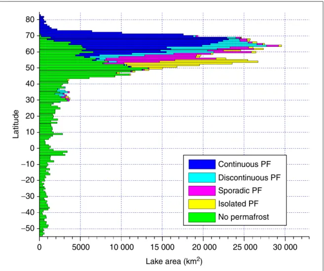
The global lake area distribution shows that a vast amount of lakes are present in the high northern latitudes (figure 3). In permafrost regions the amount of lakes is strongly controlled by thawing processes. Thawing of permafrost due to higher temperatures leads to permafrost degradation. The term thermokarst describes the resulting effects on permafrost geomorphology. Ice rich permafrost settles when it thaws and the frozen water melts. An abundant degradation feature are thermokarst lakes. They appear in depressions developed by the ground subsidence. Northern permafrost regions are occupied by tens of thousands thermokarst lakes (Grosse et al. 2013; French 2018).

Figure 3: Global lake area distribution in comparison to latitude and permafrost zones (Grosse et al. 2013)

(14)

2.2 SAR backscatter characteristics

The low albedo and good conductivity of surface water leads to heat fluxes from the water to the surrounding permafrost and increased air temperatures over the water bodies. They reach 10 °C to 12–14 °C over MAATs in central Alaska and Arctic Alaska, respectively. In warmer areas the heat flux can result in a talik below the lake and thus lateral degradation of permafrost. Depending on the permafrost thickness, thawing can progress through the layer completely (Jorgenson et al. 2010). Soil or sediment temperatures close to lakes are also raised by several degrees Celsius. Langer et al. (2016) modelled mean surface temperature deviations of +10 °C and +13 °C between soil without the presence of waterbodies (-9 °C) and soil at small waterbodies (1 °C) and soil at medium waterbodies (4 °C), respectively. Therefore, thermokarst lake development enables fast permafrost degradation compared to the relatively slow permafrost thaw without comparable features. It impacts extensive areas because of its high abundance in Arctic permafrost regions (Grosse et al. 2013).

If lakes freeze to the bottom (bedfast ice) or contain liquid water below a layer of surface ice (floating ice) has a great impact on heat transfer. Mean heat fluxes of both bedfast and floating ice are higher than those of the ambient tundra. The mean heat flux of floating ice is, however, nearly four times as high as that of bedfast ice (Jeffries et al. 1999).

2.2 SAR backscatter characteristics

Radar backscatter characteristics of frozen lakes were extensively researched for the last decades. Variations of dielectric constants between materials and surface rough- ness determine penetration properties of the radar signal. The discrimination between floating and bedfast ice is based on the different dielectric constants between the transition of ice and liquid water and ice and the lake bed (sediments). A greater change in the dielectric constant cause a higher proportion of the radar signal to be reflected.

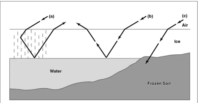
The dielectric constant of ice and frozen soil is very similar with values of 3 and 3.12, in contrast to liquid water with a dielectric constant of 60. Hence, the radar signal is absorbed by bedfast lake ice and reflected by floating ice. For a strong backscatter of the signal to the receiver elongated air bubbles play a crucial role. They are oriented in the direction of the ice growth and therefore perpendicular to the ice surface. They decrease omnidirectional scattering by transmitting the radar signal towards the ice- water transition and the reflected signal back to the upper surface of the ice. Thus, low backscatter can represent both an absence of bubbles and bedfast ice (Weeks et al.

1981; Mellor 1982). Figure 4 shows those three different circumstances in a simplified manner.

These characteristics apply to different wavelengths, incidence angles, polarisations and acquisition modes. Jeffries et al. (1994) used calibrated C-band radar with VV polarisation and field validation data from the North Slope of Alaska to quantify temporal

(15)

2.2 SAR backscatter characteristics

variations of backscatter coefficients. In autumn before an ice layer is developed on lakes, strong winds can roughen the surface and lead to high backscatter. As soon as a thin layer of ice is present backscatter decreased. Backscatter values increased as the ice was thickening until a rapid drop occurred at the lakes which were sampled as bedfast. Backscatter from floating ice was -6 to -7 dB and from bedfast ice -17 to -18 dB. Comparison of Arctic and sub-Arctic lakes shows that backscatter of floating ice is very similar while bedfast ice has a 3 dB lower backscatter in Arctic than in sub-Arctic regions. This could be because the lake bed of Arctic lakes is more likely to be frozen than that of sub-Arctic lakes where water might be still unfrozen for some time after the lake became bedfast (Morris et al. 1995).

Figure 4: Illustration of radar scattering in floating lake ice containing bubbles (a), floating lake ice without bubbles (b) and bedfast lake ice with contact to the lake bed (c) (Duguay et al. 2002)

The incidence angle of C-band radar influences backscatter intensities in particular of floating ice which has a low amount of bubbles. Lake ice with a greater amount of bubbles showed small differences of 1 dB at floating ice and 1–3 dB at bedfast ice between steeper (20–34°) and shallower (35–49°) incidence angles. Floating ice with few air inclusions, however, had a similar backscatter at shallow incidence angles to bedfast ice (Duguay et al. 2002).

In addition to the widely used C-band radar to distinguish between floating and bedfast lake ice X-band radar has also successfully been used. Jones et al. (2013) mapped floating ice using a fixed threshold to classify overwintering freshwater habitats in the Arctic Coastal Plain of Alaska with TSX radar data at a wavelength of 3.1 cm.

Detection of floating ice has an agreement with the ground data of 90.6 % and bedfast of 99.7 %. Similar success was made with TSX backscatter intensity time series in

(16)

2.3 Lake depth estimation

lakes of the Lena delta where the drop of backscatter at the time of the change from floating to bedfast was observed (Antonova et al. 2016).

A comparison between L-band radar with a wavelength of 23.6 cm and C-band radar with 5.7 cm wavelength in the northern Seward Peninsula and the Arctic Coastal Plain was done by Engram et al. (2013). L-band backscatter differences of floating and bedfast ice were not as pronounced as backscatter intensities of C-band radar. Because backscatter of floating ice was in comparison higher in C-band radar the difference between floating and bedfast ice was five to thirty-six times higher compared to single polarised HH L-band radar.

2.3 Lake depth estimation

Before calibrated SAR images were present Mellor (1982) linked bright and dark tones of X-band radar, corresponding to floating and bedfast lake ice, to bathymetric and ice thickness measurements of lakes. Thus, bathymetry of lakes without any previous depth information were achieved. Hirose et al. (2008) extracted ice thicknesses from SAR data by connecting depth soundings to the floating-bedfast boundary. This approach was not reliable as the estimated ice thickness is affected by several potential uncertainties.

Water levels during the depth soundings and acquisition dates of the SAR data could differ. Snow cover thickness influences ice growth and was not taken into account and the measured water depth was not at the precise location of the floating-bedfast boundary.

Lake ice regime classification and numerical ice growth modelling were used to either determine a broad overview about lake depth (Jeffries et al. 1996) or extract more detailed isobaths of each lake (Kozlenko and Jeffries 2000).

A number of studies used the empirical ice growth formula by Lebedev (1938) to derive ice thickness. Sea ice thickness derived from SMOS and from the Lebedev formula show good agreement (Kaleschke et al. 2012). In comparison to measured ice thicknesses, however, King et al. (2017) found that the calculated values are in three out of four studied years smaller than the measured mean. Only in the most recent year they were in the margin of the error of the measured mean. Another study including SMOS data used the formula to investigate the sensitivity of SMOS brightness temperature in respect of ice thickness (Maaß 2013). Su and Wang (2012) validated their sea ice thickness results based on MODIS data with two ice growth formulas and achieved good agreements. To use the Lebedev formula to receive lake ice instead of sea ice thickness the freezing point is elevated from -1.9 °C to 0 °C (Barry and Gan 2011).

(17)

3 Study area

3.1 Prudhoe Bay

Location and extent

148°W 148°W

150°W 150°W

69°50'N

69°50'N 140°E

180°

140°W

¯

0 5 10 20 30 40

Kilometers 1:800.000

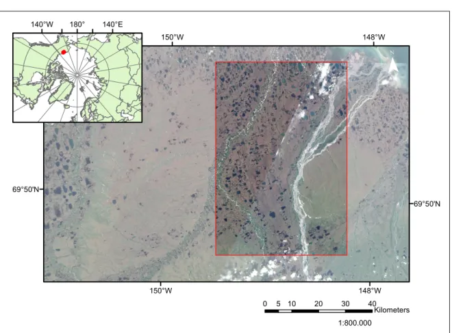
Figure 5: Location of the study area in Prudhoe Bay, Alaska (red rectangle). Background image: Sentinel 2 RGB composite mosaic image acquired on 24 and 30 July 2018 The first study area is located at the Beaufort Sea coast in the North Slope Borough between Barrow in a westward direction and the Canadian border in the East. Its extent is between 148.2° and 149.6° West and 69.6° and 70.3° North with a total area of 3546 km² (figure 5). Two rivers cross the study area from south to north with the majority of the studied lakes between them and westward of the smaller Kuparuk River in the West. The eastward and bigger River is the Sagavanirktok River.

The Prudhoe Bay oil field, which is the third largest oil field in the United States, lies in the north of the area. This results in extensive infrastructure such as roads, gravel pads, buildings and an airport which were build since the discovery in 1967 (Raynolds et al. 2014; U.S. Energy Information Administration 2015).

Climate

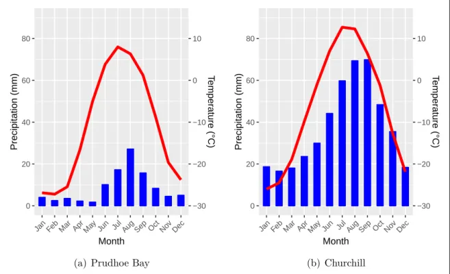
The climate station Prudhoe Bay recorded monthly mean temperatures from -27 °C in February to 8 °C in July (figure 6a). This characterises the climate as tundra climate

(18)

3.1 Prudhoe Bay

(E) on the Köppen–Geiger climate classification, where the warmest month does not exceed an average temperature of 10 °C (Köppen 1918). The mean annual temperature is -11.2 °C in the period 1981–2010. The winter temperatures are not as moderated by the sea as similar places along the Beaufort Sea coast, e.g. Barrow, because the coastal waters are frozen after mid October and mitigate the warming effect on air temperatures of the sea (Walker 1980). The annual precipitation is 102 mm with a pronounced peak in the months June to September where the mean monthly precipitation is between 10 mm and 27 mm (figure 6a). The mean annual snowfall is 84 cm with monthly averages up to 23.6 cm in October. July is the only month without snowfall (Western Regional Climate Center 2019). Polar day lasts from mid May to end July (72 days) and polar night from end November to mid January (49 days) (Walker 1980).

0 20 40 60 80

−30

−20

−10 0 10

Jan Feb Mar Apr May Jun Jul

Aug Sep Oct Nov Dec Month

Precipitation (mm) Temperature (°C)

(a) Prudhoe Bay

0 20 40 60 80

−30

−20

−10 0 10

Jan Feb Mar Apr May Jun Jul

Aug Sep Oct Nov Dec Month

Precipitation (mm) Temperature (°C)

(b) Churchill

Figure 6: Climographs of Prudhoe Bay and Churchill, average precipitation and temperature data from 1981-2010. Data from Western Regional Climate Center (2019) (Prudhoe Bay) and Environment and Climate Change Canada (2019) (Churchill)

Geomorphology and Permafrost conditions

The Prudhoe Bay area is composed of unconsolidated Quaternary sediments which consist of sands, gravel, clays and silts. Major parts of these Quaternary deposits are originated from the Tertiary Sagavanirktok Formation and relocated materials from the southern Brooks Range. They are comparable to recent terrace and bed deposits of the Sagavanirktok and Kuparuk Rivers. These deposits are overlaid with 1.5 and 2.5 m of ice rich organic matter containing silts which are again overlaid with loess deposits up to 1 m. At the surface there are organic deposits. Most of the ground ice

(19)

3.1 Prudhoe Bay

appears as segregated ice in layers or lenses due to pore water migration. Big amounts of ice are present in ice wedges which developed polygonal tundra patterns in Prudhoe Bay (Everett 1980a).

The area is mostly flat with a mean surface elevation of 9 m and relief differences of about 2 m. Exceptional cases are larger streams and pingos where relief differences can reach up to 15 m (Everett and Parkinson 1977).

Prudhoe Bay is located in the continuous permafrost zone around 500 km north of the adjacent discontinuous permafrost zone (Jorgenson et al. 2008). The permafrost depth is around 600 m below sea level (Osterkamp and Petersen 1985). The active layer thickness ranges from 20–70 cm in tundra areas and less than 20 cm in river floodplains (Liu et al. 2012). Mean annual permafrost temperature in 20 cm depth was around -6.5 °C in 2004 (Osterkamp 2007) and mean summer temperature ranges from 3.6 °C to 3.9 °C in 8 cm depth (Everett 1980a).

(20)

3.2 Churchill

Location and Extent

94°W 94°W

58°10'N 58°10'N

140°E 180°

140°W

¯

0 5 10 20 30 40

Kilometers 1:900.000

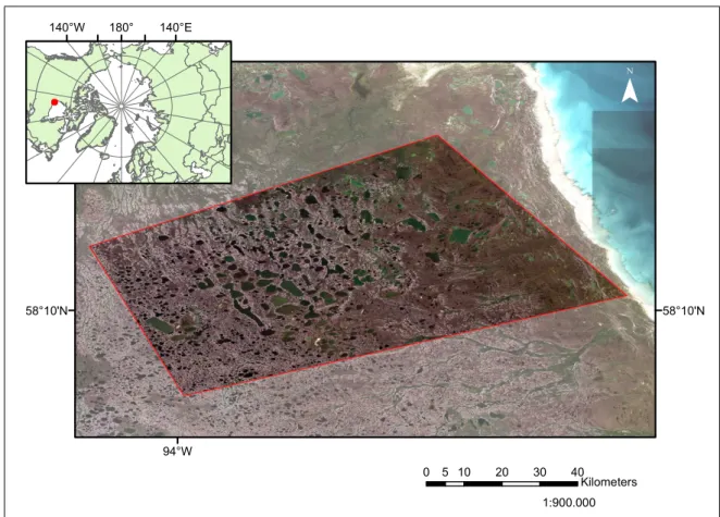
Figure 7: Location of the study area in Churchill, Manitoba, Canada (red rectangle). Back- ground image: Sentinel 2 RGB composite mosaic image acquired on 09 August and 16 September 2017

The second study area is around 40 km south of the town Churchill in northern Man- itoba, Canada. It is located on the west shore of the Hudson Bay between 92.9° and 94.2° West and 57.9° and 58.6° North with a total area of 2820 km² (figure 7). The study area is at the border of the Wapusk National Park which reaches from the coast nearly to the edge of the study area. The tundra vegetation consists mainly of shrubs, moss, lichen and fedge types. It is generally treeless except for the vicinity of river corridors (Ponomarenko et al. 2014).

Climate

The mean annual temperature in Churchill was -6.5 °C in the period 1981–2010. The coldest month is January with a monthly average of -26 °C and the warmest is July with 12.7 °C. Only four month (June to September) have an average temperature above 0 °C. With the warmest month above 10 °C and the coldest below -2 °C the Köppen–

Geiger climate classification results in a continental climate (D) (Köppen 1918). The annual precipitation is 452.5 mm with a peak in August and September (figure 6b).

(21)

3.2 Churchill

The annual snowfall is 201 cm with July and August being the only months without snowfall. Snowfall accounts for 39 % of the annual precipitation (Environment and Climate Change Canada 2019).

Geomorphology and Permafrost conditions

The area around Churchill is located on deposits from the last glaciation and the following postglacial period. The land slopes from the sea westward with a relatively even rate of 3 m/km. The area was covered by ice from the Hudson Bay which deposited silty and calcareous till. The dominant land form in the study area is polygonal tundra with a thick layer of peat accumulated during the Holocene (peat plateau). Peat thickness increases from the coast landward and is between 100 and 150 cm in eastern parts of the study area and 150 to 200 cm in western parts (Dredge and Mott 2003).

The study area is located in discontinuous permafrost close to the boundary of contin- ious permafrost in the north (Duguay et al. 2002). The mean annual ground temperature is between -1 °C and -2 °C but is dependent on the surface materials. Layers of peat insulate the permafrost according their thickness (Ponomarenko et al. 2014).

Smith et al. (2010) measured ground temperatures of two sites in Churchill located in bedrock and in a more vegetated peat richer location. The annual range of near surface temperatures and the thickness of the active layer differ much between the locations.

Annual amplitudes are 40 °C in bedrock with an active layer of 11.5 m compared to 12 °C and 3.8 m in the peat richer site. Temperature in 15 m and 10 m varied 1 °C and 0.5 °C, respectively.

(22)

4 Material and methods

4.1 Remotely sensed data

To distinguish bedfast and floating lake ice conditions in Prudhoe Bay and Churchill Sentinel 1 synthetic aperture radar (SAR) scenes from the end of the particular winters in 2015, 2016, 2017 and 2018 were used. There was no data for 2016 available covering the whole study area in Prudhoe Bay, which is why analysis of that winter was not conducted. Sentinel 1 uses C-Band radar with a frequency of 5.405 GHz and a wavelength of ~5.5 cm. The acquisition dates in Prudhoe Bay are ranging from 29 to 30 April and in Churchill from 16 to 30 April. The more consecutive scenes from January to April 2018 in Prudhoe Bay and end of December 2017 to April 2018 in Churchill were used to estimate lake depth. The majority of the data, especially in more recent years (from 2017 onwards), were dual polarisation products with vertical transmit and vertical receive (VV) and vertical transmit and horizontal receive (VH).

They were acquired in the Interferometric Wide (IW) swath mode, single look with a spatial resolution of 5 m by 20 m and a pixel spacing of 10 m. The incidence angle range is within 30–46°. The scenes in Extra Wide (EW) swath mode were dual polarisation horizontal transmit, horizontal receive (HH) and horizontal transmit, vertical receive (HV) with a 20 m by 40 m spatial resolution and an incidence angle range of 19–48° (table 1).

Additionally one Sentinel 2 scene from the 24 July 2018 for Prudhoe Bay was used to produce a lake or water mask. This was done by defining a threshold reflectance value for band 8, which corresponds to the near infrared spectral range. By visual comparison a reflection of <0.06 was defined as water. As only lakes should remain, the water which belonged to river systems was removed with a created river shape file.

The water mask for the lakes in Churchill was derived by thresholding a Sentinel 1 SAR image from 08 September 2017 as the backscatter difference between water and tundra was very pronounced. Using a Sentinel 2 product for masking gave a worse result in Churchill with more mixed pixels, especially in the shore areas of the lakes. Water bodies with an area of less than 10000 m² were sorted out to minimise classification errors due to the relatively large pixel size of 10 m (IW) and 40 m (EW) of the SAR data.

To produce radiometrically calibrated SAR images the original Sentinel 1 scenes had to be preprocessed. Preprocessing was done with the Sentinel Application Platform (SNAP), an open source architecture which combines all toolboxes from the European Space Agency. Four steps according to Veci (2016) were applied: radiometrical calibration, speckle reduction, terrain correction and conversion to decibel scaling. Calibration corrects pixel value variations between different images, e.g. due to differing incidence angles, and lead to the true backscatter. Quantitative analyses with SAR data can

(23)

4.2 Lake ice regime classification

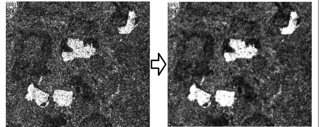
only be done after calibration. Speckle reduction or filtering reduces the noise of radar images. The refined Lee filter was chosen in this study because it gives the best performance out of the available despeckling filters in SNAP (Lukin et al. 2017). A before and after speckle filtering example is shown in figure 8.

Figure 8: Calibrated SAR image (left) and image after applying a Refined Lee speckle filter (right)

A Range–Doppler Terrain Correction was done to correct geometric distortions due to topographic features. Two different digital elevation models, depending on the region, were used to minimise the geometric effects on the image: For Churchill the SRTM Global 1 arc second dataset (Version 3.0) and for Prudhoe Bay the ASTER Global Digital Elevation Model. The final preprocessing step included the conversion to radar backscatter coefficient (σ⁰) in decibel (dB). The used equation wasσ⁰ = 10∗log10(DN), where DN indicates the value of the uncalibrated backscatter intensity (Veci 2016).

4.2 Lake ice regime classification

The corresponding lake masks were used to exclude pixels with backscatter information derived from the tundra. To distinguish between floating and bedfast lake ice an unsupervised k–means classification was done. It is an iterative clustering process which assigns each image value to one ofk classes. After a defined number of iterations each value is allocated to the class with the closest arithmetic mean (Surdu et al. 2016).

The classification was performed with the R programming language with a maximum number of 100 iterations and two classes. Each class was then manually assigned to either represent bedfast or floating lake ice conditions.

Sobiech and Dierking (2013) did comprehensive performance tests with unsupervised k–means classification and a manually defined backscatter threshold to differentiate ice and water surfaces. Both methods lead to suitable results. The best results on lakes were attained with k–means classification. The unsupervised method has the

(24)

4.3 Lake ice growth

advantage that no prior statistics of the data have to be taken as the backscatter coefficients between bedfast and floating ice are considerably different. Typical frequency distributions ofσ⁰ from lakes which have fractions of floating and bedfast ice show a bimodal pattern. K–means clustering with two classes divide these bimodal distributions approximately at the minimum between the two normal distributions.

Pixels close to the threshold can falsely be classified as the wrong lake ice regime as the two distribution overlap (Engram et al. 2018). Because the k–means classification chooses the threshold between the classes for every image separately it adapts to backscatter coefficient differences due to varying polarisations, incidence angles and meteorological and ice conditions (Sobiech and Dierking 2013). Hence, only a minimum of manual supervision is necessary in the classification process.

The classification results were converted to polygon features using ArcGIS. Total areas and areal percentages of bedfast and floating lake ice were calculated and used to classify each lake into a predominant lake ice regime. Corresponding to Arp et al.

(2012) lakes with >95 % bedfast ice pixels were assigned to bedfast and lakes with

≤95 % bedfast ice pixels to floating lake ice regime. The information of the lake ice regime for each lake and year was organised in a lake polygon shapefile based on the previously described lake mask.

The predominant lake ice regime across the years for each lake was identified using five different states: stable bedfast, stable floating, transition to bedfast, transition to floating and intermittent lakes. Stable are lakes which are classified as bedfast or floating in every year. Transitional lakes are classified as floating in the first year and bedfast in all subsequent years (transition to bedfast) or vice versa (transition to floating). Intermittent lakes have changing lake ice conditions and fit in neither of the above regimes.

4.3 Lake ice growth

Lake ice growth was calculated using a formula by Lebedev (1938)

d=a∗F DD^b, (1)

where d indicates ice thickness in cm, factor a is set to 1.33 and b is 0.58. Freezing degree days (FDDs) were calculated for temperatures below 0 °C. The equation is empirically derived from 24 station years in the Russian Arctic under average snow conditions (Maykut 1986). FDDs are defined as the cumulative sum of mean daily temperatures below 0 °C. The sum of those negative temperatures is given a positive algebraic sign (Assel 1980; Desch et al. 2017). The start date was chosen by the first day with subzero temperatures. Temperature data was derived from MODIS Land Surface Temperature and Emissivity daily data which has a spatial resolution of 1 km and provide daily daytime and nighttime surface temperatures in a 1200 by 1200 km

(25)

4.3 Lake ice growth

grid (Wan et al. 2015). Download, conversion and geographic projection was done with a Python script and further processing in R. Processing steps were masking out the relevant study areas from the grid, selecting layers with daytime and nighttime information, converting values to degree Celsius, averaging day and night to one daily temperature and linear interpolating of missing values in between the scenes.

The resulting daily FDDs for each 1 km pixel were then assigned to the closest lake in ArcGIS and converted to ice thicknesses using equation (1). For every classified SAR image the boundary between floating and bedfast lake ice was extracted similar to the procedure described in Kozlenko and Jeffries (2000). On the basis of the image acquisition dates the corresponding ice thickness was chosen as it equates to the lake depth at the boundary between bedfast and floating ice. The bedfast part of the lake is shallower than the ice thickness at that time and the floating fraction deeper. As winter progresses bigger parts of each lake become bedfast and provide more information about lake depths. The extracted boundaries were merged into one lake depth raster dataset.

(26)

4.3 Lake ice growth

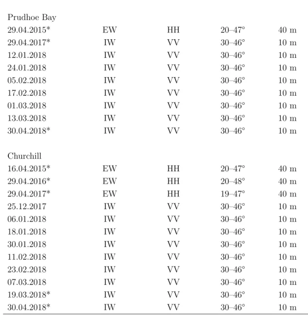
Table 1: SAR acquisition dates, modes, polarisation, incidence angle and pixel size for the data used to classify lake ice conditions for each year (marked with *) and produce lake depth estimations for 2018 in Prudhoe Bay and Churchill

Acquisition date Acquisition Mode Polarisation Incidence angle Pixel size Prudhoe Bay

29.04.2015* EW HH 20–47° 40 m

29.04.2017* IW VV 30–46° 10 m

12.01.2018 IW VV 30–46° 10 m

24.01.2018 IW VV 30–46° 10 m

05.02.2018 IW VV 30–46° 10 m

17.02.2018 IW VV 30–46° 10 m

01.03.2018 IW VV 30–46° 10 m

13.03.2018 IW VV 30–46° 10 m

30.04.2018* IW VV 30–46° 10 m

Churchill

16.04.2015* EW HH 20–47° 40 m

29.04.2016* EW HH 20–48° 40 m

29.04.2017* EW HH 19–47° 40 m

25.12.2017 IW VV 30–46° 10 m

06.01.2018 IW VV 30–46° 10 m

18.01.2018 IW VV 30–46° 10 m

30.01.2018 IW VV 30–46° 10 m

11.02.2018 IW VV 30–46° 10 m

23.02.2018 IW VV 30–46° 10 m

07.03.2018 IW VV 30–46° 10 m

19.03.2018* IW VV 30–46° 10 m

30.04.2018* IW VV 30–46° 10 m

(27)

5 Results

5.1 Prudhoe Bay

The total lake area in Prudhoe Bay is 279 km² which equates to around 8 % of the study area. 2556 lakes with respective areas of more than 10000 m² were analysed in the years 2015, 2017 and 2018.

Fractions of floating and bedfast ice pixels in regard to the total lake area for the end of each winter were calculated and the lake state for each lake was classified.

Additionally five predominant lake ice regimes were identified: Stable bedfast, stable floating, transition to bedfast, transition to floating and intermittent lakes.

Furthermore, ice growth for the winter 2017/2018 was calculated and used to estimate lake depths with the lake ice classification results.

5.1.1 Lake ice classification

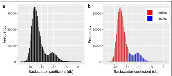
The σ⁰ frequency distribution of lakes from the 29 April 2016 is shown as an example in figure 9. Figure 9B indicates the k–means clustering outcome and shows that the threshold between bedfast and floating ice is around the minimum between the two distributions.

The average bedfast lake ice percentage in the years 2015, 2017 and 2018 was 68 %.

The distribution of each year is shown in figure 10. The highest percentage of bedfast ice was in 2015 were it reached 80 %. Especially in the northern part of the study area the majority of lake area was classified as bedfast while more floating lake ice was present in the southern part. Bedfast lake ice decreased in the following years to 66 % in 2017 and 59 % in 2018. Thus, there is a range of 21 % over the years.

0 10000 20000 30000

−20 −15 −10 −5 0

Backscatter coefficient (db)

Frequency

a

0 10000 20000 30000

−20 −15 −10 −5 0

Backscatter coefficient (db)

Frequency

bedfast floating

b

Figure 9: Bimodal frequency distribution from Sentinel 1 backscatter coefficients of lake pixels on 29 April 2015 in Prudhoe Bay; b shows the k–means clustering result with bedfast (low values) in red and floating (high values) lake ice regimes in blue

(28)

5.1 Prudhoe Bay

(a) 29 April 2015, 80% bedfast (b) 29 April 2017, 66% bedfast

(c) 30 April 2018, 59% bedfast

Bedfast ice Bedfast ice Floating ice Floating ice

Figure 10: Bedfast and floating ice pixels in April 2015, 2017 and 2018 in Prudhoe Bay

(29)

5.1 Prudhoe Bay

Table 2: Percentage of bedfast ice pixels in each year in comparison to the amount of the corresponding freezing degree days in Prudhoe Bay

Year Bedfast ice area Bedfast lakes FDDs

(percentage of lake area) (percentage of total No lakes)

2015 80 % 79 % 3617

2017 66 % 64 % 3602

2018 58 % 55 % 2996

The number of as bedfast classified lakes, with more than 95 % bedfast lake area, was very similar to the absolute amount of bedfast lake ice. It was 79 %, 64 % and 55 % for the years 2015, 2017 and 2018, respectively (table 2).

Analysis of the predominant lake ice regime in the recent years showed that half of all lakes were stable bedfast in all years. One fifth (18.5 %) were identified as stable floating. The transitional classes reveal that lakes in the transition to floating exceeded the percentage of lakes in the transition to bedfast by a factor of >16 (13.3 % and 0.8 %).

The remaining lakes with a share of 17.3 % had changing lake ice regimes and are in the class of intermittent lakes (table 3).

Table 3: Lake ice regimes in percentage of total number of lakes in Prudhoe Bay Lake ice regime Fraction (total number lakes)

Stable bedfast 50.1 %

Stable floating 18.5 %

Transition to bedfast 0.8 %

Transition to floating 13.3 %

Intermittent 17.3 %

The amount of bedfast lake ice was further compared to freezing degree days, the resulting ice thickness, mean early winter temperatures from the months October, November and December and mean winter temperatures for the period October to April (figure 11). The amount of bedfast lake ice decreased steadily in the three observation years. It followed a linear decrease (figure 11a). The values for FDDs, ice thickness and mean temperature as potential influencing factors of the fraction of bedfast ice, showed a different development during this time. They had a non linear course. There were only minor changes between 2015 and 2017. FDDs decreased from 3617 to 3602 resulting in a change of ice thickness by about 1 cm. Mean early winter and mean winter temperatures showed a similar course with increases of less than 1 °C. Between 2017 and 2018 there were bigger changes present. FDDs decreased by about 600 to 2996 and ice thickness by nearly 15 cm from 153.7 cm to 138.1 cm. Mean early winter and mean winter temperatures both increased by approximately 3 °C to -9.5 °C and -17 °C, respectively (figure 11b,c,d). The relationship between bedfast ice percentages

(30)

5.1 Prudhoe Bay

and FDDs is further shown in figure 12. The linear fit shows an increase of bedfast ice with increasing FDDs. The coefficient of determination (r²) is 0.63.

(31)

5.1 Prudhoe Bay

●

58 ●

66 80

2015 2016 2017 2018

Bedfast ice (%)

(a) Bedfast ice percentage of total lake area by the end of winter

● ●

3000 ●

3200 3400 3600

2015 2016 2017 2018

FDDs

(b) Number of FDDs at the time of lake classification

● ●

●

135 140 145 150 155

2015 2016 2017 2018

Ice thickness (cm)

(c) Estimated ice thickness from FDDs

●

● ●

●

−16

−14

−12

−10

2014/2015 2015/2016 2016/2017 2017/2018

Year

Temperature (C°)

●

OND Winter

(d) Mean temperature from winter (October to April) and the beginning of winter (October, Novem- ber, December)

Figure 11:Comparison of bedfast ice pixels, FDDs, ice thickness and early winter temperatures in Prudhoe Bay

(32)

5.1 Prudhoe Bay

●

50 65 80

3000 3200 3400 3600

FDDs

Bedfast (%)

●

Churchill Prudhoe Bay

Figure 12:Relationship between bedfast ice percentage and FDDs; r² for the linear fits are 0.04 for Churchill and 0.63 for Prudhoe Bay

(33)

5.1 Prudhoe Bay

5.1.2 Lake depth

Figure 13 shows the simulated ice growth curve from 01 September 2017 to 31 May 2018. For the purpose of illustration, it is based on MODIS temperature data which was averaged over the study area. The vertical lines display the acquisition dates from the SAR images used to estimate water depth (see table 1) and the vertical lines the corresponding ice thickness at that time. At the first acquisition date at 12 January 2018 the ice was 100 cm thick and increased by more than 60 cm over the period to the last acquisition date at 30 April 2018.

0 10 20 30 40 50 60 70 80 90 100 110 120 130 140 150 160 170

Sep 2017 Oct 2017 Nov 2017 Dec 2017 Jan 2018 Feb 2018 Mar 2018 Apr 2018 May 2018 Jun 2018

Ice thickness (cm)

Figure 13:Calculated ice growth curve from 01 September 2017 to 31 May 2018 for Prudhoe Bay; dashed vertical lines indicate SAR acquisition dates and dashed horizontal lines the corresponding ice thickness

Analysis of water depth distributions show that approximately 25 % of the water area was below 100 cm deep and already bedfast in the beginning of January. The depth ranges between 100 cm and 160 cm were relatively equal distributed: 100–120 cm accounted for 10 % and 120–140 cm and 140–160 cm accounted each for 15 %. The depth of the water area which is more than 160 cm can not further be estimated as the ice was still floating at the end of April. Hence, 35 % of all water area was deeper than 160 cm (figure 14a).

Figure 14b shows the distribution of mean water depth of the 1414 out of 2556 lakes that were classified as bedfast by the end of April 2018. The vast majority of lakes (60 %) had a mean water depth of less than 90 cm, which was the minimum ice thickness at the first acquisition date. The frequency of deeper lakes halved with every 10 cm class. Around 20 % of lakes had a depth of 90–100 cm, 10 % of 100–110 cm, 5% of 110–120 cm and 2.5% of 120–130 cm. The mean depth of the remaining lakes with

(34)

5.1 Prudhoe Bay

floating ice can not be estimated more precisely apart from that they were deeper than 130 cm.

0 20 40 60

80 100 120 140 160 180

Percentage

(a) Distribution of water depth across all waterbodies

0 20 40 60

80 90 100 110 120 130

Water depth (cm)

Percentage

(b) Distribution of mean water depth from lakes with bedfast lake ice regime

Figure 14:Distribution of water depth in Prudhoe Bay; (a) shows the overall distribution of depth referring to the total lake area and (b) the mean water depth of lakes which freeze completely to the ground

(35)

5.2 Churchill

In the study area south of Churchill lakes occupy 390 km² which accounts for 14 % of the region. The lake ice conditions of 2104 lakes were analysed in the years 2015, 2016, 2017 and 2018.

Lake depth estimations are based on the ice growth curve of the period from September 2017 to the end of May 2018.

5.2.1 Lake ice classification

The average percentage of bedfast ice was 62 % and therefore slightly lower compared to Prudhoe Bay. The highest fraction of bedfast ice was in April 2016 where it reached 74 % while it varied between 57 % and 60 % in the other years (figure 15).

Comparison of bedfast ice in regard to the total lake area and number of lakes with bedfast lake ice regimes showed deviations in both directions. The biggest difference was in 2015 where 32 % of the lakes were bedfast while the fraction of bedfast area was nearly twice as high. In the other years those values did not differ that much. In 2018 two SAR scenes with one month temporal distance were compared because of the noticeable low value of bedfast lakes of 10 % at 30 April 2018. One month earlier bedfast lakes accounted for 54 % while 10 % less total bedfast ice was detected. This was because the classification outcome of the April image was more heterogeneous and contained more noise (figure 16). Therefore, the number of bedfast lakes was disproportionately low as the threshold of 95 % bedfast ice area per lake was less likely achieved (table 4).

Table 4: Percentage of bedfast ice pixels in each year in comparison to the amount of the corresponding freezing degree days in Churchill

Year Bedfast ice area Bedfast lakes FDDs

(percentage of lake area) (percentage of total no. lakes)

2015 58 % 32 % 3471

2016 74 % 83 % 3219

2017 57 % 45 % 3148

2018 (19 March) 50 % 54 % 3044

2018 (30 April) 60 % 10 % 3572

Analysis of the ice regimes over the studied period is shown in table 5. For the reasons given above, bedfast lakes for 2018 were based on the SAR image from March. Lakes with a stable bedfast ice regime in all four observation years had a share of 13.5 % and stable floating lakes of 9.5 %. Lakes with a clear transitional regime to either bedfast or floating were poorly represented with percentages of 1.0 and 1.7, respectively. By far the most lakes (74.3 %) had a changing lake ice regime.

(36)

5.2 Churchill

(a) 16 April 2015, 58% bedfast

(b) 29 April 2016, 74% bedfast

(c) 29 April 2017, 57% bedfast

(d) 30 April 2018, 60% bedfast Bedfast iceBedfast ice Floating ice Floating ice

Figure 15: Bedfast and floating ice pixels in April 2015, 2016, 2017 and 2018 in Churchill

(37)

5.2 Churchill

The course of bedfast ice showed an increase of 16 % between 2015 and 2016 followed by a decrease of 15 % to the year 2017. Between 2017 and April 2018 there was not much change of bedfast ice (figure 17a). FDDs on the contrary decreased in the first two years but rose about 500 to the highest level of the four years between 2017 and April 2018. This leads to a weak correlation between bedfast ice percentages and FDDs (figure 12). A similar development was present in the estimated ice thickness which reached 150 cm in 2015 and decreased to 144 cm and 142 cm in 2016 and 2017, respectively (figure 17a,b). In April 2018 ice thickness was at its highest with 153 cm.

Average temperatures for early winter rose by 2.5 °C from -11 °C between the first and the second observation year and stayed nearly the same for 2016 and 2017. In the subsequent year temperature was at its lowest with -13 °C. Mean winter temperatures had a similar course but without differences between the winters of 2014/2015 and 2017/2018 (figure 17d).

(a) 19 March 2018 (b) 30 April 2018

Bedfast ice Bedfast ice Floating ice Floating ice Figure 16: Lake ice classification from 15 March and 30 April 2018 in Churchill

Table 5: Lake ice regimes in percentage of total number of lakes in Churchill Lake ice regime Fraction (total number lakes)

Stable bedfast 13.5 %

Stable floating 9.5 %

Transition to bedfast 1.0 %

Transition to floating 1.7 %

Intermittent 74.3 %

(38)

5.2 Churchill

●

50 55 60 65 70 75

2015 2016 2017 2018

Bedfast ice (%)

(a) Bedfast ice percentage of total lake area by the end of winter

●

3100 3200 3300 3400 3500

2015 2016 2017 2018

FDDs

(b) Number of FDDs at the time of lake classification

●

135 140 145 150 155

2015 2016 2017 2018

Ice thickness (cm)

(c) Estimated ice thickness from FDDs

●

● ●

●

−16

−14

−12

−10

−8

2014/2015 2015/2016 2016/2017 2017/2018

Year

Temperature (C°)

●

OND Winter

(d) Mean temperature from winter (October to April) and the beginning of winter (October, Novem- ber, December)

Figure 17:Comparison of bedfast ice pixels, FDDs, ice thickness and early winter temperatures in Churchill; the red dot indicates the value for 30 April 2018 in (a),(b)&(c)

(39)

5.2 Churchill

5.2.2 Lake depth

The simulated ice growth curve is shown in figure 18. Ice thickness was extracted at 9 SAR acquisition dates beginning at 25 December 2017. Data was available every 12 days except for the last two dates (table 1). The range of utilised ice thickness to estimate lake depth was between 90 cm and 170 cm.

Distribution of water depth across all waterbodies, i.e. not based on individual lakes, shows that around 22 % of the water area was less than 80 cm deep. The subsequent depths show a gradually increase in their distributions of about 5–6 % for every 20 cm depth class: 8 % of the water area is 80–100 cm deep, 14 % 100–120 cm, 20 % 120–

140 cm and 27 % 140–160 cm. The last class contains water area which was still floating at the end of April and therefore depth can only be estimated as more than the the ice depth at this time. It accounted for 9 % of the area (figure 19a).

Mean lake depth distribution of the 1141 lakes which were classified as bedfast on 19 March 2018 is shown in figure 19b. Most of the lakes had a mean depth of 100–120 cm (23 %), but with only a difference of a few percent to the other mean depths which accounted for 16 % and 19 % for the mean depths of 60–80 cm and 80–100 cm while 20 % and 18 % of the lakes were 120–140 cm and 140–160 cm deep. The remaining 4 % of the lakes had a mean water depth between 160 cm and 180 cm.

0 10 20 30 40 50 60 70 80 90 100 110 120 130 140 150 160 170 180

Sep 2017 Oct 2017 Nov 2017 Dec 2017 Jan 2018 Feb 2018 Mar 2018 Apr 2018 May 2018 Jun 2018

Ice thickness (cm)

Figure 18:Calculated ice growth curve from 01 September 2017 to 31 May 2018 for Churchill; dashed vertical lines indicate SAR acquisition dates and dashed horizontal lines the corresponding ice thickness

(40)

5.2 Churchill

0 10 20 30 40

60 80 100 120 140 160

Percentage

(a) Distribution of water depth across all waterbodies

0 10 20 30 40

60 80 100 120 140 160 180

Water depth (cm)

Percentage

(b) Distribution of mean water depth from lakes with bedfast lake ice regime

Figure 19:Distribution of water depth in Churchill; (a) shows the overall distribution of depth referring to the total lake area and (b) the mean water depth of lakes which freeze completely to the ground

(41)

6 Discussion

6.1 Methodical limitations

Different sources of errors due to the used methods are identified. One is due to the fact that the chosen unsupervised k–means classification works with statistical differentiations of the values. This leads to misclassified pixels if their backscatter difference is not sufficient. A potential reason could be a relatively small amount of air bubbles in the ice which decrease the backscattered signal from floating ice. SAR images with shallow incidence angles as used for 2015 in Prudhoe Bay and 2015–2017 in Churchill (HH Polarisation) are more affected by that effect (Duguay et al. 2002). This could cause the fraction of bedfast ice to be overestimated. Misclassification of bedfast ice, however, can occur if there is unfrozen sediment (talik) present at the bottom of the lake according to Grunblatt and Atwood (2014). The unfrozen sediments would provide an ice–water transition with a strong dielectric contrast similar to the effect at floating ice.

The accuracy of lake ice classification depends further on the lake mask. It is derived from a single year and does not adapt to potential lake size changes and shoreline shifts in between the years. Furthermore, it includes all water as it is based on the reflection of near infrared for Prudhoe Bay and radar backscatter for Churchill. In a second step, rivers were excluded manually and small river fractions could be present in the final lake mask. Additionally location inaccuracies between the lake mask and the SAR scenes lead to mixed pixels. This impacts especially SAR images in Extra Wide (EW) swath mode as the pixel size is 40 m opposed to Interferometric Wide (IW) swath mode with a pixel size of 10 m. Those mixed pixels occur on the lake shores where the signal respond is both from the tundra and the water surface. Tundra has usually backscatter intensities similar to floating water wherefore the margin around bedfast lakes could be falsely classified as floating. The impact of mixed pixels on the classification accuracy is bigger for small lakes as they include fewer total pixels.

The exclusion of small waterbodies of less than 10000 m² should minimise this effect.

However, lakes of that size consist of just 100 pixels in IW swath mode (100 m² pixel area) and 6 pixels in EW swath mode (1600 m² pixel area).

The ice growth curve is based on the empircal equation by Lebedev (1938). It is a very simplistic approach which takes only temperature development in the form of freezing degree days into consideration. The other components of the equation are constant.

Temporal variations apart from temperature which influence ice growth are averaged over the observation time and the area the equation was derived from. Variation in snow cover thickness is therefore neglected but it affects ice growth considerably and is found to be the most important factor on ice thickness variation in the Arctic (Zhang and Jeffries 2000) as a thicker snow cover insulates the ice layer and reduces ice growth

(42)

6.2 Evaluation of the results

speed (Wei et al. 2016). The average snowfall conditions used for the formula are not exactly known and it can not be determined reliably if the ice growth curve is generally overestimating or underestimating ice thicknesses in this study.

6.2 Evaluation of the results

The bedfast ice fractions of 57–80 % depending on the year and study area are in the range of previous studies from Arctic regions. Long term observations showed values from less than 40 % to around 50 % in the outer Arctic Coastal Plain in the period from 2003 to 2011 (Arp et al. 2012). Near Barrow, Alaska, bedfast ice varied between 26 % and 62 % from 1992 to 2011 (Surdu et al. 2014). Engram et al. (2018) analysed lakes over 25 years in 8 different areas in Alaska and obtained bedfast ice fractions from as low as 10 % up to 90 % in some years. The area closest to Prudhoe Bay has bedfast ice between 60 % and 90 %. A large scale circumpolar investigation by Bartsch et al. (2017) in 50 x 50 km grid cells results in 60–100 % fraction of bedfast ice for that region.

In Prudhoe Bay bedfast ice decreased over the study period constantly. The comparison with freezing degree days, ice thickness and winter temperature indicates that the proportion of bedfast ice is not a simple function of temperature. Lake depth is probably not equally distributed so that a certain rise in temperature does not lead to a defined decrease in bedfast ice. Hence, sensitivity analyses of bedfast ice in regard of the response to climatic conditions is more complex. It can be assumed that tipping points exist which cause sudden changes once they are exceeded rather than linear relationships. The observation period is too short to recognise trends in bedfast ice. Arp et al. (2012) and Surdu et al. (2014) hypothesised more floating ice regimes and less bedfast ice fractions, respectively, based on much more extensive observation periods compared to this study. However, those trends could not be confirmed by analysis of temporal patterns of even more years (Engram et al. 2018). It is therefore very likely that bedfast ice fractions increase again in subsequent years. Additionally the percentage for 2016 is missing which could have changed the pattern considerably. However, as there is a relationship between bedfast ice percentages and FDDs it can be assumed that a decreasing amount of FDDs in the future lead to less bedfast ice. Simulated temperature projections for northern Alaska show an increase in annual mean temperature of 4.2–6.4 °C, depending on the emission scenario, for the period 2070–2099 in respect of 1971–1999. Winter temperatures (December to February) are predicted to rise to most (around 7 °C), which should have a substantial effect on FDDs and therefore bedfast ice occurrence (Stewart et al. 2013).

The above mentioned uncertainty due to the short observation time applies also to the identified predominant lake ice regimes in Prudhoe Bay. In this study half of the lakes were stable bedfast in all observations years and around one fifth floating. The lakes