1
Implementation of a code for Dynamical Mean Field Theory with Exact Diagonalization as Impurity solver
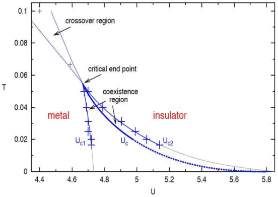
The purpose of the exercise is to build a DMFT code for the one-band Hubbard model using Exact Diagonalization as impurity solver. The self-consistent solution should then be analyzed changing the parameters of the model. The phase diagram of reference can be seen in the Figure below.
The folder with all necessary files can be copied from the home directory of usercms00:
cp -R ~cms00/ED_DMFT-2011 .
Figure 1: QMC phase diagram (from Bl¨umer PhD Thesis 2003). The half-bandwidth D is here equal to 2.
2
mini How-To
1. The loop begins with filelisadiag.andparcontaining, exactly as we did in Exercise 2, the starting Anderson parameters (use just a, possibly educated, guess).
2. As in Exercise 2, lisadiag.datand lisadiag.input contain the other necessary parameters.
3. To get the impurity Green’s function on the Matsubara frequencies (iωn =iπT(2n+
1)) at each iteration, the Anderson Impurity Model (AIM) code we worked with during Exercise 2 can be used. It is also possible to use the version of lisadiag.f provided here. The only thing to change is the definition of the frequencies: Now the Green’s function on the Matsubara axis is needed, instead of on real frequencies as it was for Exercise 2. Either all or positive frequencies only, can be used. The two places where this has to be done are marked by “?? Matsubara ??”.
4. the solution of the AIM yields lisadiag.greencontaining G(iωn).
5. the DMFT self-consistency condition for the Bethe lattice case reads
G0(iωn)−1=iωn+µ− D2
4 G(iωn)
whereDis the half-bandwidth. This equation can therefore be used to get the “new”
G0(iωn).
IMPORTANT: This has to be written on the file G0w.dat, which is needed by the programfit.f. The format of such file is described below, as well as programfit.f.
Additionally, to avoid possible oscillations between different solution during the DMFT loop, it would be desirable to mix the “new” G0(iωn) - before writing it to the file G0w.dat - with, e.g., the non-interacting Green’s function of the AIM, namely
GAnd0 (iωn)−1=iωn+µ−X
k
Vk2 iωn−ǫk
Alternatively, the G0(iωn) of the previous step can be used for the mixing.
6. From the “new”G0(iωn), the “new” Anderson parameters can be obtained through a fitting procedure. This can be done using the small programfit.fprovided here.
Program fit.fcan be compiled in the following way:
gfortran -fbounds-check -O fit.f -o FIT.x
3
It looks into lisadiag.dat to initialize several arrays. Recompiling is necessary every time N s and/or Iwmax are changed in file lisadiag.dat. The code also reads the Anderson parameters from lisadiag.andparand the chemical potential from lisadiag.input. These three files are expected to have the same format as those used during Exercise 2 for the AIM code.
7. As we already said,fit.fneeds file G0w.dat to readG0(iωn) from. This file has to contain Iwmax(defined in lisadiag.dat) lines and three columns: The (real part of the) Matsubara frequency in the first column, and the real and imaginary part of G0(iωn) in the second and third columns.
8. The output offit.fis a new set of Anderson parameters, contained in filenew.andpar.
The format is the same as lisadiag.andpar, so simply copying new.andpar into lisadiag.andparwill be enough to start over with a new iteration.
9. To check whether self-consistence has been reached, the AIM Green’s functionG(iωn) can be plotted as a function of the iterations. When the changes in both the real and the imaginary parts ofG(iωn) between to consecutive iterations are negligible, a self- consistent solution has been reached. A saturation in the values of the Anderson parameters as a function of the iteration also indicates that self-consistency has been reached. More quantitative estimates of the convergece parameter would give unambiguous results, but are not really needed in this context.
Typically, of the order of 10-20 iterations are enough to converge, unless too few Anderson parameters are used or unless there is a phase transition or a critical point close by. In those cases more iterations are needed, and the intial guess for the Anderson parameters becomes important.
10. A consideration about the values of the Anderson parameters: These are deter- mined by a multi-dimensional fit ofG0(iωn) with the functional formG0And(iωn)−1 = iωn+µ−P
k Vk2
iωn−ǫk. This has no unique solution and since many regions of the parameter space can have shallow minima, tiny differences coming from rounding errors can give different results for the final set of the Anderson parameters. This makes comparisons between different implentations of the self-consistency loop a bit complicated. However, the values of the Anderson parameters have no physical meaning individually. Physical quantities like, e.g. the Green’s function, will depend much less on these small differences.
4
About the exercise
You are free to choose your favorite metod (fortranXX, C, C++, shell scripts, Mathemat- ica, Matlab,...) to implement the self-consistency equation in order to get G0(iωn) and build the rest of the DMFT loop calling program lisadiag.fand programfit.f.
To check your results, you can set the half-bandwidthD in the self-consistency condition (pag. 2, step 5.) to 1 and use the input parameter files contained in theED DMFT-2011di- rectory (lisadiag.dat,lisadiag.inputandlisadiag.andpar). After 15 iterations, you should get something very similar to the Green’s function contained in lisadiag.green, corresponding to the Anderson parameters contained in lisadiag.andpar.15
For each set of converged Anderson parameters you can get the spectral function making an additional run of the AIM code on the real axis (as in Exercise 2). This will give a nice visualization of your metallic or insulating solution, characterized, respectively, by the presence of a quasi-particle peak at the Fermi level or of a spectral gap
Further developments of the exercise, for those who choose this as topic for the final talk, are:
• study the coexistence region around the first-order phase-transition line (see Figure 1)
• calculate the self-energy at self-consistency:
Σ(iωn) =G0And(iωn)−1−G(iωn)−1
A diverging Σ(iωn) at low-frequencies corresponds to an insulating solution, while a (linearly) vanishing Σ(iωn) for ωn→0 corresponds to a metallic solution.
• implement the self-consistency equation for a different density of states than the semicircular one
• study the behavior of physical quantities like, e.g. double occupations, to character- ize the phase diagram