Dynamical Mean Field Theory

(1)

of

inhomogeneous correlated systems

Inaugural-Dissertation

zur Erlangung des Doktorgrades der

Mathematisch–Naturwissenschaftlichen Fakultät der Universität zu Köln

vorgelegt von

Rolf Helmes

aus Siegen

K¨oln 2008

(2)

Berichterstatter: Prof. Dr. Achim Rosch Prof. Dr. Matthias Vojta

Tag der m¨undlichen Pr¨ufung: 14.01.2008

(3)

Abstract

In the last one and a half decade, the Dynamical Mean Field Theory (DMFT) allowed to get insight into the Mott metal-insulator transition (MMIT) and many long-standing questions about the nature of the transition could be answered, at least in the limit of infinite dimensions. In this thesis, the adaption of the DMFT to inhomogeneous systems is studied, opening the possibility to study a rich variety of systems and challenging physical questions. Firstly, the basic problem is studied, how a metal penetrates into a Mott insulator, where analytically found power-laws at the critical point can be confirmed with numerics. Secondly, the phase separation between metal and insulator is investigated, which can occur since the MMIT is a first order transition. The spontaneous build up of domains is observed in numerical simulations and the domain walls are examined. Finally, the MMIT of fermionic atoms in an optical lattice is studied.

Kurzzusammenfassung

Die Dynamical Mean Field Theory (DMFT) hat in den letzten 15 Jahren einen Einblick in den Mott-Metal-Isolator Übergang (MMIT) ermöglicht, und viele lang ausstehende Fra- gen über die Art des Übergangs konnten beantwortet werden, zumindest im Limes von unendlich vielen Dimensionen. In dieser Arbeit wird die Adaption der DMFT auf inho- mogene Systeme untersucht. Dies eröffnet die Möglichkeit, eine Reihe an interessanten physikalischen Fragestellungen zu bearbeiten. Zunächst wird das grundlegende Problem untersucht, wie ein Metall in einen Mott-Isolator eindringt, wobei analytisch gefundene Potenzgesetze am kritischen Punkt numerisch bestätigt werden können. Anschließend wird die Phasenseparierung zwischen Metall und Isolator studiert, die aufgrund der Natur des MMIT als Übergang erster Ordnung auftreten können. Die spontane Ausbildung von Domänen wird in numerischen Simulationen beobachtet und die Domänenwände werden analysiert. Schließlich wird der MMIT von fermionischen Atomen in einem optischen Gitter untersucht.

3

(4)

(5)

Chapter 1 Introduction

The fermionic Mott transition at temperature T = 0 is simple to explain on a very basic level. It is the consequence of the competition of the two parts of the fermionic Hubbard model. One part describes the hopping of fermions – let us consider spin-1/2 electrons – on a lattice. Focusing on three dimensions and pushing aside issues like superconductivity or nesting, one can identify the eigenstates of the hopping term as a Fermi liquid, i.e. a metal. The second part of the Hubbard Hamiltonian accounts for the on-site repulsion U of two electrons with opposite spin on the same site. Allowing only for a uniform hopping t and restricting the system to be half filled, it is intuitively clear that upon increasingU/t a transition from the Fermi liquid to an insulating state must occur. For U/t ≫ 1, the on-site repulsion suppresses the hopping and one obtains the Mott insulator.

Regarding the transition at finite temperatures T > 0, the situation becomes more complex. In contrast toT = 0, no clear differentiation between the metal and the insulator is possible. However, if one considers phases at temperatures T sufficiently below the critical temperature T_c of the second order end point and close to the transition line, one can clearly distinguish between two different thermodynamic phases, a “bad metal” and a

“bad insulator”. The “bad insulating” state is thermally activated and has a finite density of states at the chemical potential. In this thesis we will be rather sloppy and refer to the “bad metal” as “metal” and to the “bad insulator” as “Mott insulator”. Here, a too intuitive picture might be misleading. The concept of the Mott insulator as a half- filled lattice, where the isolated electrons are localized since the cost U of hopping to an occupied neighboring site is too high, is too naive and neglects the strongly correlated nature of the state. If this concept proved true, adding a single electron to the Mott- insulator would result in the metallic state, since the electron could move freely on top of the other electrons. At T > 0, this concept is oversimplified. The statistic ensemble of the Mott-insulating state always contains double occupied sites, yet it can clearly be distinguished from a thermodynamically different metallic state. Furthermore, at T > 0, the Mott insulator is stable against a small doping.

From this discussion one already realizes that rich and interesting physics appears from the innocent looking Hubbard model, which is the prime example and also the minimal model for materials where strong correlations play a role. In three dimensions, no exact

7

(8)

analytic method exists to describe the Mott transition. In the late 1980s and early 90s the Dynamical Mean Field Theory (DMFT) was developed which is able to analyze the transition in the approximation of neglecting spatial fluctuations. The method becomes exact in the limit of infinite dimensions d. In analogy to the Weiss mean-field theory of the Ising model, the DMFT singles out one site of the lattice and absorbs all other sites into a non-interacting bath coupled to the considered site. While in the Weiss mean- field theory the bath is described by a single parameter, the effective magnetic field, the bath in the DMFT is described by a frequency-dependent bath function which represents an effective density of states for an electron tunneling out of the single considered site.

Thereby dynamic processes as electrons tunneling away and back to sites are captured by the DMFT. The effective model is the Anderson impurity model, consisting of an impurity – the singled out site – which is coupled to a non-interacting bath. The DMFT was able to elucidate the transition for d=∞. For the paramagnetic case where magnetic ordering is neglected, the Mott transition turns out to be a first order transition, which has two second order endpoints: one atT = 0 and one at critical temperatureT =Tc. The resulting phase diagram is artificial. Regarding generic materials, below a certain critical temperature the system will pass over into an antiferromagnetic ordered Mott insulator below the Neel temperature TN. However, TN can be lowered by frustrating the lattice which suppresses the magnetic ordering.

Let us return to the question raised above: how does a Mott insulator react to adding electrons, i.e. doping? The issue was only settled recently for a uniform system in the DMFT approximation and neglection of Coulomb forces, see Chapter 4. At 0< T < Tcand increasing doping, the system passes through the first order phase transition at a critical chemical potentialµ_c, displaying the typical physics of phase separation. Since particle-hole symmetry is broken by finite doping, the metallic and the insulating phase have different fillings. Thus a macroscopic separation of domains is impeded by the Coulomb force. To treat the possible scenario of a microphase separation in Chapter 4, the usual DMFT method needs to be generalized to treat inhomogeneous systems, as explained in Chapter 2. In contrast to the homogeneous DMFT, where all sites are assumed to be in the same state, in the inhomogeneous case the sites of the lattice are intrinsically different, resulting in different bath functions for different sites. Thus many instead of one Anderson impurity models need to be solved.

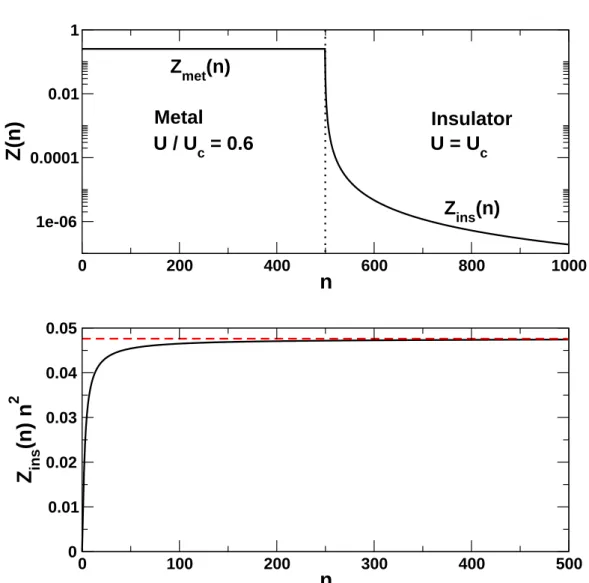
The idea of neighboring metallic and insulating domains raises the very basic question of how a metal penetrates into a Mott insulator. Considering an explicit inhomogeneous system consisting of a metal with Umet < Uc and a Mott insulator with Uins > Uc, where Uc is the critical interaction for a given hopping t, the behavior of the system close to the junction has not been clarified so far. In Chapter 3, we investigate this problem. We find that the relevant energy scales in the Mott insulator are the coupling J ∝ t²/U of the spins of the localized electrons, which competes with the quasi-particle weight Z of the penetrating metal, corresponding to the Kondo temperatureTK in the impurity model.

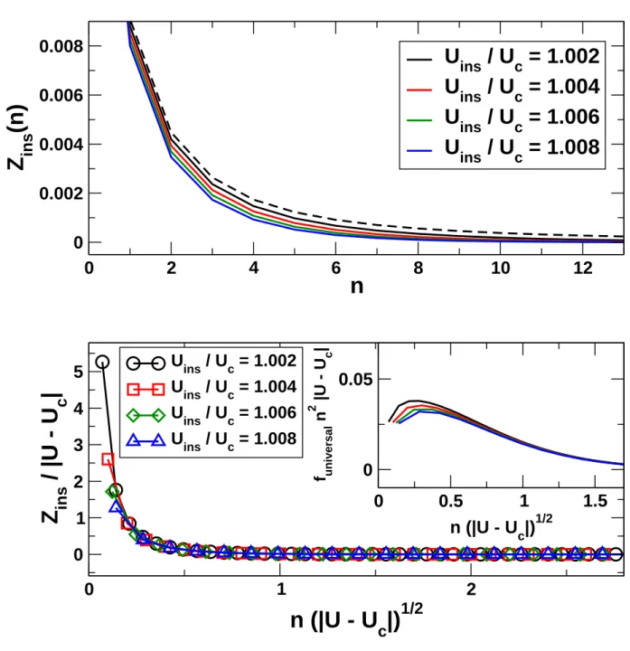
Since we neglect magnetic order and regard a paramagnetic system withJ = 0, we find that the metal penetrates infinitely deep into the Mott insulator. By varying the interaction Uins and the temperature T, we study the universal scaling behavior around the second

(9)

order end point Uins=Uc and T = 0.

In Chapter 5, the Mott transition of fermionic atoms in an optical lattice is studied.

In order to confine the atoms, an external potential is needed which makes the problem inhomogeneous. Naturally the occupation vanishes approaching the border of the trap.

Hence the bordering regions can be conceived as a strongly doped material and are certainly metallic. Depending on the depth of the trap, the center will be double occupied and band insulating. The band insulator will be surrounded by a strongly doped metallic region.

If the on-site interaction is strong enough, a half-filled Mott-insulating region appears between the two metallic regions. Here the issue discussed in Chapter 3 is very relevant:

since the metallic regions penetrate into the insulating regions, the results presented in Chapter 5 differ considerably from calculations done in a local density approximation, a method widely used in the literature.

(10)

(11)

Chapter 2 Model and Method

2.1 The Hubbard model

The physics of electrons in a solid is described by the general Hamiltonian H=H0+Hee

[1, 2], where

H0 = Z

d^dra^†_σ(r) pˆ²

2m +V(r)

a_σ(r), Hee = 1

2 Z

d^drd^dr^′Vee(r−r^′)a^†_σ(r)a^†_σ′(r^′)aσ^′(r^′)aσ(r). (2.1) Here, the degrees of freedom of the ions of the lattice have been neglected and the interaction of the ions with the electrons has been simplified by introducing an effective lattice potential V(r). The first part H0 describes the one-particle physics of electrons moving in the lattice potential while Hêe describes their interaction via the Coulomb force. Despite its innocent appearance, the Hamiltonian 2.1 describes an abundance of solid state physics phenomena. Unfortunately, it is impossible to make further progress without simplifying it by making further approximations. For many materials, the following approach is very successful. Using the density functional theory [3] combined with the local density approximation (LDA), one can absorb the ionic potentialV(r) and the electron-electron Coulomb interaction Hêe into an effective potential veff, arriving at the Kohn-Shahm equation, a one-particle Schrödinger equation for the electrons,

H^effφj(r) =

−∇²

2m +Veff(r)

φj(r) =εjφj(r). (2.2) Here φj(r) is a complete basis set of one-particle states. By Fourier transforming to k−space one obtains the band-dispersion ǫ^k of the electrons. Then Heff takes the form P

kǫkc^†kσckσ. If one rewrites H⁰ in the Wannier state basis,

|ψ^Rni ≡ 1

√Nsites

X

G∈B.Z.

e⁻ⁱ^G^·^R|ψ^kni, (2.3) 11

(12)

one obtains

Heff =X

i,i^′

tii^′c^†_iσci^′σ, (2.4) where tii^′ = _N¹

sites

P

keⁱ^k⁽^Rⁱ⁻^R^i′⁾ǫk and Nsites is the number of sites in the lattice. Here we consider only a single band and neglect all others, thus we have dropped the band index.

This Hamiltonian has the simple interpretation of electrons hopping between lattice sites, where tii^′ is the amplitude for hopping between the lattice sites i and i^′.

For materials where the true electron-electron interactions play an important role, the approach above is insufficient and needs to be extended. In 1963, Hubbard, Gutzwiller and Kanamori introduced the celebrated fermionic Hubbard model [4–6],

H −µNˆ =−µX

i,σ

c^†_i,σc_i,σ+ X

<i,j>,σ

t_i,jc^†_i,σc_j,σ+UX

i

n_i,↑n_i,↓, (2.5) where we have introduced the chemical potential µ and the particle number operator ˆN. Here the interaction term Un_i,↑n_i,↓ = Uc^†_iσc^†_i′σ^′cjσcj^′σ^′ has been introduced to model the Coulomb repulsion of two electrons on the same site. The Hubbard model is the prime example and also the minimal model for highly correlated electrons on a lattice. By “correlated” one does not refer to the usual symmetry correlations of fermions but to correlations between the electrons caused by the interaction term, which is crucial for the displayed physics of the model. In the following we will only consider lattices with dimensions higher than one, since physics in one dimension exhibits many peculiarities compared to physics in higher dimensions (Fermi-liquid theory is not applicable and replaced by Luttinger liquid theory, including spin-charge separation, etc.). At U/t = 0 the Hubbard model describes a metal with independent Bloch electrons moving in a band determined by the dispersion ǫk = P

i,jeⁱ^k⁽^Rⁱ⁻^R^j⁾tij. This in principle easy problem might get more complicated if one desires to describe materials where band structure calculations are necessary to compute the dispersionǫ^k. However, here we will make the further simplification of assuming a uniform hopping, tij ≡ t, and consider simple lattices where the dispersion can be calculated analytically. The Hubbard model studied in this thesis thus takes the form

H=t X

<i,j>,σ

c^†_i,σc_j,σ+UX

i

ni,↑ni,↓. (2.6)

If nesting is neglected and assuming that one is far from instabilities like superconductivity, for small U/t≪ 1 the free electrons are renormalized according to Fermi liquid theory developed by Landau in 1956-58, see, e.g. Ref. [7, 8]. In the other limit, i.e.

U/t≫1 and in the case of a lattice with half fillingn = 1/2, the Hubbard model describes the so-called Mott insulator as hopping is suppressed by the large Coulomb repulsion of the electrons [9]. The only degrees of freedom left are the spins of the electrons at each site and the Hubbard model can be mapped to the Heisenberg model,

H^Heisenberg =J X

<i,j>

Sˆi·Sˆj, (2.7)

(13)

with J ∝t²/U [2]. This is a problem of quantum magnetism, where spin wave theory can be applied around the anti-ferromagnetic ground state. Thus for both limits U/t≪1 and U/t≫1 theories and methods exist to describe the Hubbard model. However, we already see that at some intermediate interaction a transition from metal to insulator, termed

’Mott-Hubbard metal-insulator transition’, must occur. So far, an analytical method to describe this transition is not in sight and the best way to tackle the physics of the transition is a numerical method called ’Dynamical Mean Field Theory’ which will be described in the next section.

In Chapters 3 and 4 we will be concerned with two physical problems motivated by experiments with highly correlated electrons, which can be described by the Hubbard model. Chapter 5 deals with a completely different physical scenario, optical lattices.

Here, the Hubbard model is realized by fermionic atoms confined in an optical lattice, see Section 5.1.

2.2 Dynamical Mean-Field Theory (DMFT)

2.2.1 Method

As mentioned above, an analytic solution for the Hubbard model (2.6) is out of sight and one has to retreat to numerical methods to investigate the Mott-Hubbard metal-insulator transition. A breakthrough has been achieved with the ’Dynamical Mean Field Theory’

(DMFT), which is able to resolve the first order transition from metal to insulator, see Fig.

2.1 for the case of a half-filled lattice. In the following we will only consider paramagnetic solutions and any magnetic order will be neglected. This can either be seen as a crude approximation calling for redemption at a later stage of the theory or one could argue that one regards a completely frustrated lattice. We will therefore drop the spin indices of the Green’s functions. The DMFT method and its approximations will shortly be described in this section.

The DMFT was developed in the late 1980s and and early 1990s. Pioneering work was done by Metzner and Vollhardt [11] and M¨uller-Hartmann [12–14]. Further development was made by Georges and Kotliar [15] and Jarrell [16]. For a comprehensive review see Ref. [10]. Let us start presenting the DMFT by shortly sketching the idea, presented in Fig. 2.2: in the interacting lattice, one site is singled out and all other sites are mapped into a bath. Thus the lattice model is mapped to an to an “impurity” model, consisting out of one single interacting site (“impurity”), which is coupled to the non-interacting bath. By solving the impurity model, one obtains the state of the single site. Assuming a translational invariant lattice, the state of the single site is now assumed to hold for all sites, thus defining the state of the lattice. The procedure is repeated until a self-consistent solution is reached.

The Hubbard model, the lattice model considered in this thesis, will be mapped to an Anderson impurity model (AIM) in the DMFT self-consistency loop. Before explaining the DMFT algorithm in more detail, let us first present the AIM, see also, e.g., Ref. [17]

(14)

Figure 2.1: Generic phase diagram (as a function of temperature T and interaction U in units of half the bandwidthD) for the Mott-Hubbard metal-insulator transition for a half- filled, fully frustrated lattice. The transition is first order, the two phases are separated by a coexistence region between Uc1 and Uc2 (dashed lines) where hysteresis effects can occur. The actual first-order transition takes places at the solid line, which terminates in two second-order end points (the end-point at T = 0 is also second order). Picture taken from Ref. [10].

for more details. The AIM is represented by the Hamiltonian H^Anderson =X

σ

ǫ0σc^†_0σc0σ +Un0↑n0↓+X

k,σ

Vk

c^†k,σc0σ+c^†_0σckσ

+X

k,σ

˜

ǫkc^†kσckσ, (2.8) where in the first two terms describe the local level with energyǫ_0σ and Coulomb interaction U. The third term describes the coupling of the impurity to a non-interacting band, which is given by the last term. The coupling of the impurity to the band can be described by the hybridization function ∆(ω) [17], where

∆(ω) = X

k,σ

|Vk|² ω−˜ǫk

. (2.9)

The local free (U = 0) Green’s functionG0(ω) can be written as

G0⁻¹(ω)≡ω+µ−∆(ω). (2.10)

Thus the interacting Green’s function G_Anderson takes the form

G_Anderson= 1

ω+µ−∆(ω)−Σ(ω), (2.11)

(15)

where the local self-energy Σ(ω) has been introduced. The AIM can be solved numerically, see Section 2.4.

The self-consistency loop can be written as Σ→^1. Glat

→ G2. 0

→3. Σ, (2.12)

which will now be explained in more detail. We start from the solution of the AIM, which is contained in the self-energy Σ(ω). Now the approximation of the DMFT enters by assuming that the lattice self-energy is local and thusk-independent and can be set equal to the self-energy of the impurity, Σlattice(k, ω) ≈ Σ(ω). Thus the on-site lattice Green’s function is given by (first step of (2.12))

Glat(ω)≡Glat(x= 0, ω) =X

k

eⁱ^xkGlat(k, ω) = Z

dǫ ρ(ǫ)

ω+µ−ǫ−Σ(ω), (2.13) whereρ(ǫ) =P

kδ(ǫ−ǫk) is the density of states of the band. The self-consistency condition can be phrased as G_lat =G_Anderson, i.e. one demands the lattice and the impurity Green’s functions to be equal, which defines the mapping of the lattice to the impurity model. The self-consistency equation can be written as

G⁻_lat¹(ω) = G0⁻¹(ω)−Σ(ω). (2.14) The free Green’s function of the impurity modelG0(ω) encodes the information of the bath of the single site, constituted by all other lattice sites. It corresponds to the effective Weiss field in the Weiss mean-field theory for the Ising model. Instead of the static Weiss field, our effective field has the form of a function, hence the method was termed dynamical mean-field theory. The ’Weiss-function’ G0(ω) will be referred to as ’bath function’ in the following. By Eq. (2.14), the bath of the Anderson impurity model, defined byG0⁻¹, can be computed with Glat and Σ (second step of (2.12)). In Section 2.4 two “impurity solvers”

will be introduced, that can be fed with G0⁻¹(ω) and will finally calculate Σ(ω) (third step of (2.12)). Thus the loop is closed and can now be iterated until a self-consistent solution is reached.

Two approximation have been made. Firstly, the solution has been assumed to be homogeneous and translational invariant. In the next section we will show how the method can be generalized to deal with inhomogeneous systems and solutions. Secondly, the self- energy has been assumed to be local, Σ(ω,xi,xj) = Σ(ω)δi,j. Metzner and Vollhardt [11]

showed that this approximations becomes exact in the limit of infinite dimensions, d→ ∞. To ensure that kinetic and interaction energy in the Hubbard model stay of the same order of magnitude while taking the limit, one has to scale the hopping as t → ^√^t^∗_z, where z is the connectivity of the lattice, which also goes to infinity as d → ∞. In this limit it can be shown that all non-local contribution are suppressed by a factor ^√¹

d. This result was obtained from a diagrammatic perturbation expansion of the self-energy in real space [11]

and in momentum-space [13], see also [10].

(16)

0000000000000000000 0000000000000000000 0000000000000000000 0000000000000000000 0000000000000000000 0000000000000000000 0000000000000000000 0000000000000000000 0000000000000000000 0000000000000000000 0000000000000000000 0000000000000000000 0000000000000000000 0000000000000000000 0000000000000000000 0000000000000000000 0000000000000000000 0000000000000000000 0000000000000000000 0000000000000000000

1111111111111111111 1111111111111111111 1111111111111111111 1111111111111111111 1111111111111111111 1111111111111111111 1111111111111111111 1111111111111111111 1111111111111111111 1111111111111111111 1111111111111111111 1111111111111111111 1111111111111111111 1111111111111111111 1111111111111111111 1111111111111111111 1111111111111111111 1111111111111111111 1111111111111111111 1111111111111111111

Figure 2.2: Dynamical-Mean-Field Theory: one site (red) of the interacting lattice is singled out. All other sites of the lattice are mapped to a bath coupled to the single site, thus the procedure maps the lattice model to an Anderson impurity model. In case of a homogeneous, translational invariant system the procedure is the same for every lattice site.

Another limitation of the method is the solution of the Anderson impurity model. Since no analytical solution exists, one has to retreat to numerical methods. Therefore DMFT can only be pursued numerically. Furthermore, all available impurity solvers are limited by their individual approximations, which affect the whole DMFT procedure, see section 2.4.

Regarding computational demands, DMFT can be done nowadays on a usual desktop PC (AMD Athlon, 3 GHz, 2 GByte RAM). The bottleneck concerning computational time and precision is step three of the self-consistency loop (2.12), which depends on the choice of the impurity solver. In the case of Numerical Renormalization Group (NRG), see section 2.4.2, which is one of the most accurate methods, the solution of the Anderson impurity model takes 1-2 minutes. In order to reach a self-consistent solution, the DMFT self-consistency loop has to be iterated around 100-1000 times, which results in a total computational time of several hours up to a day in the case of NRG. In contrast to NRG, which requires only very little memory, other impurity solvers like exact diagonalization require not only computational time but also much memory, i.e. one is either limited by computational time or memory. The other steps in (2.12) neither require a significant time nor memory.

2.2.2 Results

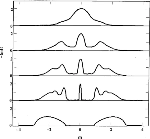
DMFT makes it possible to study the metal-insulator transition quantitatively. Results computed with the Numerical Renormalization Group (see Section 2.4.2) as impurity solver are shown in Fig. 2.3 and Fig. 2.4. As mentioned above, for small values of the interaction U we expect a Fermi liquid state with a quasi-particle resonance. The low-frequency

(17)

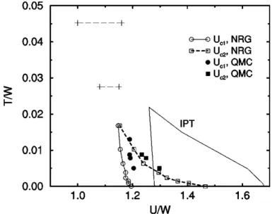
Figure 2.3: Phase diagram of the paramagnetic Mott metal-insulator transition. The temperature T and interaction U are given in units of the full bandwidth W = 2D.

Regarding the critical interactions Uc1 and Uc2, the agreement between the DMFT/NRG and DMFT/Quantum Monte Carlo results is rather good, while DMFT/IPT overestimates the Uc1 and Uc2. Picture taken from [18].

behavior of the self-energy is then given by ReΣ(ω+i0) = Un+

1− 1

Z

ω+O(ω³),

ImΣ(ω+i0) ∝ −ω²+O(ω⁴), (2.15)

c.f. Fig. 2.3, where n is the filling and Z is the weight of the quasi-particle peak [10].

Note that at zero temperature T = 0, the height of the peak is pinned to the noninter- acting value of the density of states,

A(ω = 0) =ρ(µ₀), (2.16)

where µ0 is the chemical potential at U = 0 which is determined by the filling. This was shown by M¨uller-Hartmann [12] by the following argument. In the limit of infinite dimensions, i.e. in the DMFT limit, the Luttinger theorem [12] takes the simple form

µ=µ0+ Σ(ω= 0). (2.17)

Note that ImΣ(ω = 0) = 0 at T = 0. If this result is plugged into Equation (2.13), A(ω) = (−1/π)ImGlat(ω+iδ) = ImR

dǫρ(ǫ)/(ω+µ−ǫ−Σ(ω)), one obtains Equation (2.16). Thus, atT = 0, Z is proportional to the width of the peak.

(18)

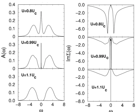
Figure 2.4: Metal-insulator transition at zero temperature calculated with DMFT and the Numerical Renormalization Group as impurity solver, see Section 2.4.2. In the left panel the spectral densities A(ω) for half filling and increasing values of the interaction U are shown. The top panel shows the metallic state with the quasi-particle peak at the Fermi-energy. Close to the transition (middle panel) the quasi-particle peak has almost vanished, whereas in the bottom panel the insulating state is reached. In the right panel the corresponding imaginary parts of the self-energies are depicted. Picture taken from [19].

By the mapping of the lattice onto the Anderson impurity model in the self-consistency loop, the energy scale ZD (where D is half the bandwidth) is translated into the Kondo temperature TK of the defined impurity problem. If the temperature T < TK, the Kondo resonance appears, which translates back into the quasi particle peak in the lattice model.

Thus whether T < TK or not decides if the considered system is metallic or insulating, respectively. Through the self-consistency loop, the Kondo resonance enhances itself, since the quasi-particle peak also appears in the bath coupled to the impurity and TK increases with the width of the quasi-particle peak in the bath. This fact is important to understand the hysteresis in the first order metal-insulator transition, see Fig. 2.1. If one starts in the metallic regime and increases U, Z and accordingly TK decrease until a critical value Uc2

is reached where Z = 0 and TK = 0. However, if one starts in the insulating regime and

(19)

Figure 2.5: Inhomogeneous Dynamical-Mean-Field Theory: for an inhomogeneous system without translational invariance the mapping from the lattice to the impurity model is different for each site. However, one still can use symmetries of the inhomogeneous lattice.

In this very simple example, the four sites at the corners and the four sites between the corner sites are equivalent. Thus there are only three different impurity models.

decreases U, no quasi-particle peak appears at Uc2 since there is no sufficient density of states at the chemical potential. The state stays metallic until the lower critical value U_c1 is reached. The real first order transition line lies in between, where the free energies of the metallic and insulating state are the same, Fmetallic=Finsulating.

2.3 Dynamical Mean-Field Theory for inhomogeneous systems

If one considers an inhomogeneous Hubbard-like model (see Sections 3 or 5) or an inhomogeneous solution of the homogeneous Hubbard model (see Section 4), the DMFT procedure has to be generalized in a way suggested by Potthoff and Nolting [20]. Before presenting Potthoff’s derivation of the mean-field equations [21], let us first explain the algorithm below. Furthermore, the approach was used by Okamoto and Millis [22]. The mapping procedure from the lattice to the impurity model becomes now different for each site, see Fig. 2.5. Thus, one generally obtains a different impurity model for each lattice site.

Depending on the specific problem under consideration, the number of impurity problems can be significantly reduced by using symmetries of the lattice. In the toy example of the 9 lattice sites in Fig. 2.5, there are only three types of inequivalent lattice sites: the four sites at the corners, the four sites between the corner sites and the one in the middle. The self-consistency loop can now be written as

{Σi}→^1. Gˆlat(i, j)→ G^2. ^0,i → {^3. Σi}. (2.18) Instead of only one self-energy we have now a set of self-energies {Σi}, one for each inequivalent site. Since translational invariance is broken, the Green’s function of the lattice can not be diagonalized by Fourier transform. In the Wannier state basis|ii, whereilabels the site, the inverse of the free Green’s function is given byG⁻¹_0,lat(i, j, ω) = hi|ω+µ−H0|ji. HereH0 is the non-interacting part of the Hubbard model. This can be written in matrix

(20)

Σ

1

Σ

2

Σ

N

G

⁻¹_lat

=

ω+ε+

t

2

Σ

1

Σ

2

Σ

3

Σ

4

Σ

N

Σ

¹

Σ

²

Σ

³

Σ

⁴

Σ

^N

G

_lat

=

invert for every

ω

G

11

22

NN

3 4

1 N

G G G G G

easy to parallelize

1.)

2.)

3.)

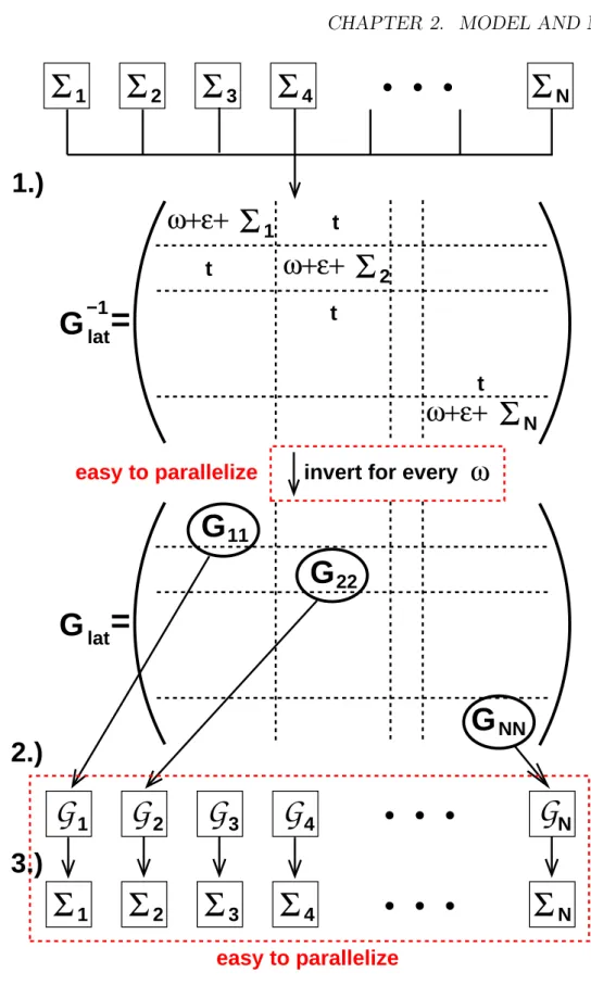
Figure 2.6: DMFT flow: the three steps of equation (2.18) are visualized. In a numerical realization of the DMFT self-consistency loop, the computations in the dashed boxes are the bottle-necks of the algorithm. Since they are independent of each other, they can be implemented very efficiently with almost no numerical overhead using parallel computing.

(21)

form

Gˆ⁻_0,lat¹ (ω) =







ω+µ t t

t ω+µ t

t ·

· t t ω+µ







, (2.19)

where the rows and columns correspond to the lattice sites and neighboring sites are connected by the hopping amplitude t. In the interacting case a self-energy matrix ˆΣ(i, j) has to be subtracted. Now again the approximation enters that the self-energy is local, Σ(i, jˆ ) ≡ Σiδi,j, i.e. off-diagonal terms of the self-energy are neglected. Thus the full Green’s function can be written as the following matrix,

Gˆ⁻_lat¹(ω) =







ω+µ−Σ1(ω) t t

t ω+µ−Σ2(ω) t

t ·

· t

t ω+µ−ΣN(ω)







, (2.20)

whereN is the total number of sites. In this notation the self-energies of symmetry related sites are the same, i.e. the self-energy of the inequivalent site i might enter the matrix several times, according to the degeneracy of site i. However, using group symmetry the matrix can be reduced such that the self-energies {Σi} of the inequivalent sites appear only once. This accomplishes the first step of the self-consistency loop (2.18) and presents the generalization of Eq. (2.13). The self-consistency condition (2.14) of the homogeneous case now takes the formGlat(i, i, ω) =GAnderson,i, i.e. the Green’s function of the Anderson impurity model of the inequivalent site i is set equal to the diagonal term of the lattice Green’s function at site i. With the help of the definitions (2.11) and (2.9) this can be written as

G⁻_lat¹(i, i, ω) =G0,i⁻¹(ω)−Σi(ω), (2.21) which presents step two of (2.18). To close the self-consistency loop, we need to solve the Anderson impurity models defined by the bath functions G0,i(ω). This will give us a new set of self-energies {Σi} (step three of (2.18)).

In contrast to the homogeneous case, the DMFT procedure for inhomogeneous systems described here is from a computational point of view very demanding, see Fig. 2.6, rep- resenting a visualization of the self-consistency loop (2.18). There are two bottlenecks.

Firstly, the computational time needed to invert the lattice Green’s function matrix Eq.

(2.20), which needs to be done for each value of the discretized ω interval, grows as N³, where N is the dimension of the matrix. Depending on the problem under consideration specifying the form and the size of the matrix, the inversion needs several seconds. For a typical discretization of the ω interval with 1000-4000 values, a total time of order of hours is needed. Secondly, the number of Anderson models which needs to be solved is

(22)

now equal to the number of inequivalent sites, typically a number about 100. In the case of NRG as impurity solver, this amounts up to several hours. Altogether, one iteration of the self-consistency loop now takes typical between four and six hours. Thus a complete run now takes a time of order of weeks. However, looking at the flow diagram Fig. 2.6, one sees that both bottlenecks can easily be tackled by parallelizing the program. Since the amount of computational time spent in the bottlenecks almost sums up to the complete computational time, the parallelization overhead is very little and the total time can be divided by the numbers of nodes used on the parallel cluster.

A very nice derivation of the DMFT mean-field equations and an illuminative view on the DMFT in general can be found in Ref. [21] by Potthoff. He introduces a general Hamiltonian H = H0(t) +H1(U) with the first part describing the hopping t and the second part describing the interaction,

H=X

α,β

tα,βc^†_αcβ +1 2

X

α,β,γ,δ

c^†_αc^†_βcγcδUα,β,γ,δ, (2.22) where α, β, ... are an orthonormal and complete set of one-particle basis states. The corresponding one-particle Green’s function takes the matrix form G_αβ(iω) = hhc_α;c^†_βii. It can be calculated from the self-energy Σα,β(iω) via the Dyson equation, which in matrix notation readsG=G0+G0ΣG, where also the free Green’s functionG0 = 1/(iω+µ−t) has matrix form, due to the hopping matrix t. Using the Legendre transform F[Σ] ≡ φ[G[Σ]]−Tr (ΣG[Σ]) of the so-called Luttinger-Ward functionalφ[G], one can write the grand potential of the system as

Ωt[Σ]≡Trln

− G⁻₀¹−Σ₋1

+F [Σ]. (2.23)

Here the subscript tindicates that Ω explicitely depends ontvia the free Green’s function G0. One can show that the grand potential Ωt[Σ] is stationary at the exact physical self-energy,

∂Ωt[Σ]

∂Σ = 0⇔G[Σ] = G⁻¹₀ −Σ₋1

. (2.24)

If one knew the grand potential explicitely, the self-energy could be determined by Eq.

(2.24). However, in general the functional F [Σ] is not known explicitely. The idea is the following: one constraints the domain of Ωt[Σ] to a subspace of self-energies for which one can find an explicit expression for Ωt[Σ]. On that subspace, Ωt[Σ] is minimized to find the best approximation to the exact self-energy. One can derive an explicit form of Ωt[Σ]

on a constrained subspace in the following way. If one wishes to find an approximation of the self-energy for the Hamiltonian (2.22), one chooses a subspace Σ(t^′), where the Σ(t^′) parametrize the exact self-energies of a set of Hamiltonians of reference systems H^′ = H⁰(t^′) +H¹(U) with the same interaction but different hopping as in (2.22). The crucial observation is thatF [Σ] does only depend on the interactionH1(U) [21]. Thus the grand potential Ωt′[Σ] of the reference system has the form

Ωt′[Σ] = Trln

−

G^′−₀¹−Σ−1

+F [Σ], (2.25)

(23)

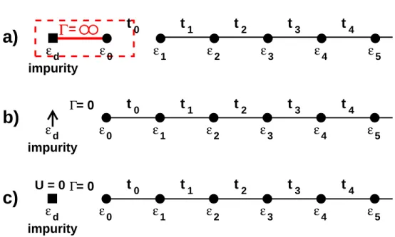
Figure 2.7: (a) Schematic representation of the Hubbard model. (b) By introducing ns

(here ns = 4) decoupled sites per lattices site, on can ceate an equivalent model. (c) By changing the hopping but keeping the same interaction, a reference system can be set up.

Forns → ∞, one obtains a model consisting out of decoupled Anderson impurity problems.

Picture taken from [20]

with the same F [Σ] as in (2.23). Thus F [Σ] can be eliminated by taking the difference, Ωt[Σ] = Ωt′[Σ] + Trln

− G⁻₀¹ −Σ₋1

−Trln

−

G^′−₀¹−Σ₋1

. (2.26)

On the subspace of the Σ(t^′), which are the correct self-energies of the reference systems H^′ =H0(t^′) +H1(U), Ωt′[Σ] is the exact grand potential Ω^′ of the system. Furthermore

G^′−₀¹−Σ−1

=G^′, the exact Green’s function of the reference system, Ωt[Σ(t^′)] = Ω^′+ Trln

− G⁻₀¹−Σ(t^′)₋1

−Trln (−G^′). (2.27) This is the main result. Note that Ωt[Σ(t^′)] only involves quantities from the reference system, apart from the free Green’s function G0. If the reference system is chosen such that quantities can be calculated easier than in the original system, one can find an approximation for Σ(t) by determining the stationary point of Ωt[Σ(t^′)], ∂Ωt[Σ(t^′)]/∂t^′ = 0, which gives

TX

ω

X

α,β

1

G⁻₀¹−Σ(t^′) −G^′

α,β

∂Σα,β(t^′)

∂t^′ = 0. (2.28)

In our case the original system is the Hubbard model (2.6), depicted in Fig. 2.7 a.

Introducing a numberns of decoupled non-interaction sites per original lattice site creates an equivalent model (Fig. 2.7 b, where ns = 4). By changing the hopping, a possible reference system can be obtained (Fig. 2.7 c). Note that for ns → ∞, the reference system consists out of decoupled Anderson impurity models. The self-energy is local, hence ∂Σij(t^′)/∂t^′ ∝δij. Thus (2.28) reduces to