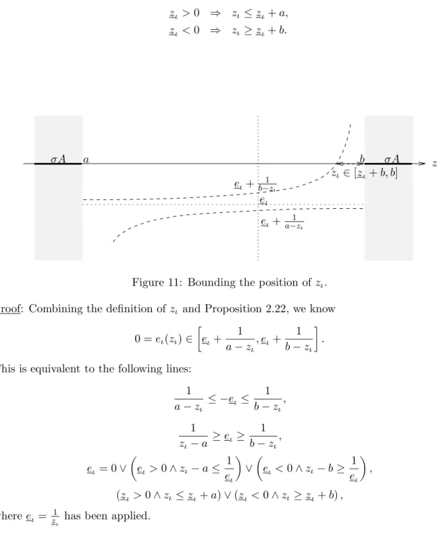
Diploma Thesis (reconstructed)

(1)

Diploma Thesis (reconstructed)

Bernhard Bodenstorfer

Some questions of the theory of perturbation of selfadjoint operators

Original 1996-02-23. Reconstructed 2010-12-09.

A note to the reader interested in the printed original version (all others may swiftly proceed to the next page):

The original printed paper version of the diploma thesis is publicly available at

• Vienna University of Technology Library (http://www.ub.tuwien.ac.at/)

• Austrian National Library (http://www.onb.ac.at/)

under the title “Some questions of the perturbations of selfadjoint operators”.

The content of the following pages is the result of an attempt to reconstruct the diploma thesis for “Technische Mathematik” as it was accepted at the Vienna University of Technology in 1996. As the original printable files have subsequently been deleted, there are some minor differences between this version and the actually printed and submitted original version:

The reconstructed work is based on the original set of L^ATEX-files, but the generation anew of the printable files has resulted in different page breaks and page numbers. (Note that the numbering of sections, propositions, formulae and the like has not changed.) Moreover, a few minor typographic errors have been corrected, none of which affected the meaningful essence of the results, however.

The upgraded version of the program gnuplotused slightly different defaults, in particular con- cerning the dimensions of some of the images.

Last but not least, all C-programs had to be ported to and executed on a different platform than what had been used for the orginal thesis. That is why the NAG-library subroutine f02faf was replaced by the LAPACK subroutine dsyevand the NAG-library subroutine d01ahfby the NETLIB (http://www.netlib.org/) implementation of dqag. (The text still mentions the originally used NAG-subroutines.) The results look essentially identical, but cleaner than the originals. The reason for the improvement is that in the process of porting the C-programs, the treatment of values close to the singularity in Cauchy principal value integrals has been slightly improved en passant.

Finally, the pre-release title of the thesis should be mentioned:

“On Compact Perturbations of Selfadjoint Linear Relations”

(2)

DIPLOMARBEIT

Some questions of the theory of perturbation of selfadjoint operators

ausgef¨uhrt am

Institut f¨ ur Analysis, Technische Mathematik und Versicherungsmathematik der Technischen Universit¨at Wien

unter Anleitung von

o. Univ. Prof. Dr. Heinz Langer

durch

Bernhard Ernst Bodenstorfer

1170 Wien, Buchenweg 3

(3)

Introduction

If a selfadjoint linear operator A in a Hilbert-space is compactly changed, the spectrum may possess additional eigenvalues afterwards in comparison to the set σpA of eigenvalues of A.

Beattie and Fox in their paper [3], study three kinds of change of A, all in the finite dimensional case: extension, modification, and restriction.

The present piece of work studies a one-dimensional extension, and the general modification by compact operators. Instead of “modification” the terminus “perturbation” is used here.

In Section 1, multiplication operatorsA on anL²-space are extended by one dimension. The eigenvalues of the extension ˜A are studied. The one-dimensional setting has the advantage of making a quick access possible even to eigenvalues which lie in the spectrum of the original operator. Therefore the intention of this section is to give an impression of the behaviour of these eigenvalues, when a real parameter is canged. This parameter specifies different extensions of the same multiplication operator.

In Section 2, a selfadjoint linear operator or relationAis perturbed by a compact selfadjoint operator T. The eigenvalues of A+T which lie in the resolvent set ρA of A are considered.

It is examined how many eigenvalues these may be and where they may occur. It is known from Weyl’s Theorem that the essential spectra of A and A+T are the same. Hence those eigenvalues can only have accumulation-points in the spectrum σA of A. By the methods proposed, a correspondence between the eigenvalues ofA+T inρAand those ofT is established which yields explicit bounds for the distance of these eigenvalues ofA+T fromσA. The bounds are similar to those which can be obtained via a min-max principle, but they apply as well for eigenvalues ofA+T inside gaps (a, b)⊆ρAof A.

Section 3 contains a study of a special kind of perturbation, and Section 4 offers a set of particular numerical examples.

Conclusively, let me devote a word of thankfulness to Prof. Langer for his advice and inde- fatigable patience which he offered to me when this piece of work was carried out. It was as well him who succeeded in raising some financial support from the Fonds zur F¨orderung der Wissenschaftlichen Forschung.

I do not want to miss to thank my parents, too, who enabled and encouraged me to follow my various studies.

Vienna, February 23, 1996 Bernhard Bodenstorfer

(5)

1 One-dimensional extension of the multiplication operator y 7→

u · y

Definition 1.1 In the following, letI ⊆IR be a set of real numbers, and letµbe some positive measure onI. ForL^pµ(I), 1≤p≤ ∞, we shall writeL^pµ. Ifµis the Lebesgue-measure (µ(t) =t), then we only writeL^p forL^pµ.

Let abe a real number, letu∈ L^∞µ be real-valued, and letv∈ L²µ be complex-valued.

The numberadefines the one-dimensional linear operatorz7→azon C, vthe linear operator C→ L²µ :z 7→zv, andu defines the multiplication operator y 7→u·y on L²µ. Byv^∗ we denote the adjoint ofv, that is L²µ→C :y7→^RIyvdµ.

Then we define the operator ˜A₁ by

A˜₁= a v^∗ v u

!

(1) on C⊕L²µ equipped with the inner product

* c₁ y₁

! , c₂

y₂

!+

=c₁c₂+ Z

I

y₁y₂dµ.

Obviously, ˜A1 is a selfadjoint bounded operator. It is a one-dimensional extension of the multiplication operatory7→u·y.

Proposition 1.1 If for a number z∈C both Z

I

|v|²

|u−z|²dµ <∞ (2)

and

z−a+ Z

I

|v|²

u−zdµ= 0, (3)

hold¹, or if²

L²µ(u⁻¹({z}))⊖Cv6={0} (4) holds, z is eigenvalue of A˜₁. Conversely, for every eigenvalue z of A˜₁, both conditions (2) and (3), or the single condition (4) hold.

The condition that both (2) and (3) hold implies the existence of an eigenvector 1 y₁

!

∈ C⊕L²µ.

1In case that fort∈I it holdsu(t−z) =v(t) = 0, the integrands ⁰₀ have to be thought to be 0. This becomes clear from the proof below. Surely, ifu(t) =zbutv(t)6= 0 for alltout of a set of positive measureµ, the integrals in (2–3) diverge, and therefore both of these conditions are violated.

2Throughout this whole work,u⁻¹({z}) means{t∈ Du: u(t)∈ {z}}. This notation is used in the same sense for other sets than{z}and other functions thanu.

(6)

Proof: Let us write “for allmost all t ∈ I with respect to the measure µ” in symbols as ∀^µ t.

Furthermore, let us agree upon the precedence ruleT₁∧T₂∨T₃=T₃∨T₁∧T₂ = (T₁∧T₂)∨T₃. We fix z∈C. Then a pair c

y

!

∈C⊕L²µ is a nonzero eigenvector of ˜A₁ if and only if the following equivalent expressions hold true:

• c y

!

6

= 0 ∧ (a−z)c+v^∗y= 0∧ ∀^µt: cv(t) + (u(t)−z)y(t) = 0

• c= 0 ∧ y6= 0 ∧ v^∗y= 0∧ ∀^µt: (u(t)6=z ⇒ y(t) = 0)

∨ c6= 0∧ (a−z)c+v^∗y= 0∧ ∀^µt:

u(t) =z ∧ v(t) = 0 ∨ u(t)6=z ∧ y(t) = −cv(t) u(t)−z

• c= 0 ∧ y6= 0 ∧ v^∗y= 0 ∧ µu⁻¹({z})∩y⁻¹(C\{0})= 0

∨ c6= 0 ∧ (a−z)c+v^∗y= 0

∧ ^µ∀t:

(u(t) =z ⇒ v(t) = 0) ∧

u(t)6=z ⇒ y(t) = −cv(t) u(t)−z

• c= 0 ∧ y∈ L²µ(u⁻¹({z}))\ {0} ∧ v^∗y= 0

∨ c6= 0 ∧ (a−z)c+v^∗y= 0

∧ ^µ∀t: (u(t) =z ⇒ v(t) = 0) ∧ ∀^µt:

u(t)6=z ⇒ y(t) = −cv(t) u(t)−z

Now we join ∃y∈ L²µ from left to all lines in thought and continue:

• c= 0 ∧ ∃y∈ L²µ(u⁻¹({z}))\ {0} ∩ {v}^⊥

∨ c6= 0∧ ∀^µt: (u(t) =z ⇒ v(t) = 0)

∧ ∃y∈ L²µ: (a−z)c+v^∗y= 0∧ ^µ∀t:

u(t)6=z ⇒ y(t) = −cv(t) u(t)−z

• c= 0 ∧ L²µ(u⁻¹({z}))⊖Cv6={0}

∨ c6= 0∧ ∀^µt: (u(t) =z ⇒ v(t) = 0)

∧ ∃y₀∈ L²µ: (a−z)c+v^∗y₀= 0 ∧ y₀(u⁻¹({z})) ={0}

∧ ∀^µt:

u(t)6=z ⇒ y₀(t) = −cv(t) u(t)−z

• c= 0 ∧ L²µ(u⁻¹({z}))⊖Cv6={0}

∨ c6= 0∧ ∀^µt: (u(t) =z ⇒ v(t) = 0)

∧ ∃y₀∈ L²µ: ∀t∈I : y₀(t) =

( 0 . . . u(t) =z

−cv(t)

u(t)−z . . . u(t)6=z ∧ (a−z)c+v^∗y₀= 0

• c= 0 ∧ L²µ(u⁻¹({z}))⊖Cv6={0}

∨ c6= 0∧µv⁻¹(C\{0})∩u⁻¹({z})= 0 (5)

∧ Z

I\u⁻¹({z})

|v(t)|²

|u(t)−z|²dµ(t)<∞ ∧ a−z+ Z

I\u⁻¹({z})

|v(t)|²

u(t)−zdµ(t) = 0

(7)

• c= 0 ∧ L²µ(u⁻¹({z}))⊖Cv6={0}

∨ c6= 0 ∧ Z

I

|v(t)|²

|u(t)−z|²dµ(t)<∞ ∧ a−z+ Z

I

|v(t)|²

u(t)−zdµ(t) = 0,

where, in the last line, we have to interpret ⁰₀ = 0 for the case u(t)−z = v(t) = 0, confer to footnote 1.

The function y₀ is defined by y₀(t) =

( y(t) . . . u(t)6=z

0 . . . u(t) =z . Note that then v^∗y₀ = v^∗y if

µ

∀t: (u(t) =z⇒v(t) = 0). This fact has been used at the upmost occurence ofy0 in the above

lines. ♥

Remark 1.1 Because ofL²µ(u⁻¹({z}))⊖Cv = ker((y 7→u·y)−z)∩kerv^∗, condition (4) can be written as ker((y7→u·y)−z)∩kerv^∗ 6={0}. That is the reason why Proposition 1.1 can be viewed as a direct consequence of the more general and elegant Proposition 2.1 to follow later on.

Moreover, Proposition 1.1 reminds us of [1, Behauptung 1], which yields only a weaker statement however, because points z with µ u⁻¹({z}) > 0 have to be excluded from the consideration there.

Remark 1.2 The properties of y and of y₀ imply y−y₀ ∈ L²µ(u⁻¹({z}))⊖Cv. That is why dim ker( ˜A₁−z) = 1+dimL²µ(u⁻¹({z}))⊖Cvif forz∈C (2) and (3) hold. This can be interpreted in the following way: A one-dimensional extension ofy7→u·y can raise the multilpicity ofz as an eigenvalue maximally by one.

Again, Proposition 2.1 together with Proposition 2.3 will show that this observation is no accident.

Remark 1.3 The eigenspace of ˜A₁ for an eigenvalue z for which (4) holds includes the space L²µ(u⁻¹({z}))⊖Cv.

This space equals that eigenspace if (2) or (3) does not hold.

For µ(t) =t, the spaceL²µ(u⁻¹({z})), and thus the spaceL²µ(u⁻¹({z}))⊖Cv is either zero- or infinite dimensional. Hence, numbers z, for which (4) holds are then eigenvalues of infinite multiplicity.

Definition 1.2 The µ-essential range of a functionu is

R^µessu=ⁿz∈C : ∀ε >0 :µ(u⁻¹(z^′ ∈C :|z^′−z|< ε ))>0^o. With this notion we can formulate

Proposition 1.2 σ(y7→u·y) =Rµessu.

(8)

Proof: We define Mε =u⁻¹({z^′ ∈C :|z^′−z|< ε}).

Let z be in R^µessu. Then, for ε > 0, we have µ(Mε) > 0. To avoid complications when µ(M_ε) =∞, chose a family of subsets M_ε¹ ⊆M_ε such thatµ(M_ε¹) = min(1, µ(M_ε)).

In order to show thatz is in σ(y7→u·y) we define a family ofL²µ-vectors by yε(t) =

( √ ₁

µ(M_ε¹) . . . t∈M_ε¹ 0 . . . t /∈M_ε¹ . It holds

kyεk²= Z

M_ε¹

1

µ(M_ε¹)dµ= 1, but also

k(u−z)yεk² = Z

M_ε¹

|u(t)−z|²

µ(M_ε¹) dµ(t)≤ Z

M_ε¹

ε²

µ(M_ε¹)dµ(t) =ε². Hence,yε6→0 but (u−z)yε →0 if ε→0. Consequently z∈σ(y7→u·y).

Conversely, assume z /∈ Rµessu. Then there is an ε₀ >0 such that µ(M_ε₀) = 0. So we have for all y∈ L²µ:

k(u−z)yk² = Z

I|u(t)−z|²|y(t)|²dµ(t) = Z

I\Mε0

|u(t)−z|²|y(t)|²dµ(t)

≥ Z

I\Mε0

ε₀²|y(t)|²dµ(t) = Z

I

ε₀²|y(t)|²dµ(t) =ε₀²kyk².

Thus,z∈ρ(y7→u·y). ♥

Remark 1.4 Directly from Proposition 1.2, it can be seen thatRµessu is a closed set.

Proposition 1.3 σessA˜₁ =σess(y7→u·y).

Proof: The essential spectrumσess

0 0 0 u

!

=σess(y7→u·y) does not change under compact perturbation (Weyl’s Theorem, see e.g. [RS, Theorem XIII.14]). ♥

1.1 Eigenvalues of A˜₁(a) outside R^µessu

This section is devoted to the study of the movement of eigenvalues z /∈ Rµessu of the operator A˜1(a) = a v^∗

v u

!

depending on the real parameter a. The operator ˜A₁(a) is already familiar from the preceding section.

(9)

It should be noted that results obtained for ˜A1(a) can easily be translated into similar results for the operator

A˜_1v(b) = a bv^∗ bv u

! . This operator describes a coupling problem, see Section 3.

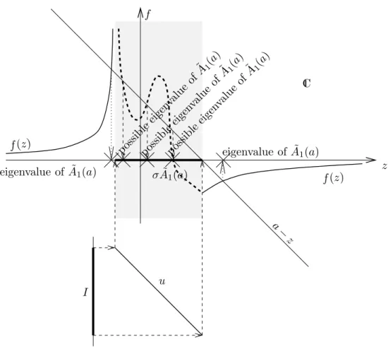
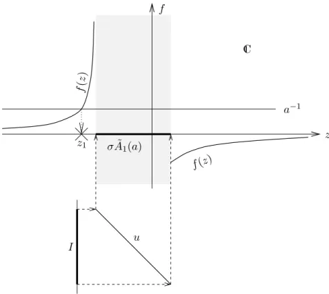
Using the function

f(z) = Z

I

|v|²

u−zdµ, (6)

condition (3) can be written as

f(z) =a−z. (7)

This functionf is holomorphic outsideR^µessu. Obviously,f is monotonous forz in any convex subset of IR\Rµessu, especially forz > Rµessu or z <Rµessu.

Proposition 1.4 If a > Rµessu holds, then there exists exactly one eigenvalue z₊ > Rµessu, and z+ ≥aholds.

Additionally, one eigenvalue may exist in each convex subset of IR\Rµessu. Further eigenvalues, if any exist, lie in Rµessu.

The case a <R^µessu is wholly symmetric.

Proof: If R^µessu < z < a, then z+f(z) < z < a holds, but z+f(z) → +∞ for z ր ∞. Hence, by continuity of f on IR\Rµessu, there is a numberz > Rµessu fulfilling z+f(z) = a.

This is an eigenvalue of ˜A₁(a), because (2) trivially holds for z /∈ Rµessu. It is the only one in (maxR^µessu,+∞), becausez7→z−a+f(z) is strictly monotonous.

In the same way, monotony of this function is the reason that in no convex subset of IR\Rµess

can be more than one numberz such that (7) holds. ♥

Remark 1.5 The assertion of Proposition 1.4 can be adapted to the casea= maxRµessu: First assume f = 0.³ Then we trivially get thata itself is eigenvalue of ˜A₁(a), becausea+f(a) =a under these circumstances. In this case we have to admit z₊ = maxRµess as the desired eigenvalue of ˜A1(a).

If f 6= 0, then it holds f ≤ −ε on (a, a^′) for some a^′ suitably near a, and for some ε > 0.

Hence, z−a+f(z)<0 for a < z < a^′. On the other hand, z−a+f(z)→ +∞ forz→ +∞. Consequently, there is a z > asuch thatf(z) =a−z.

Application of the Implicit function Theorem on (7) yields

Proposition 1.5 All eigenvalues of A˜₁(a) outside R^µessu obey the differential equation dz

da = 1

1 +^R_I _(u^|₋^v^|_z)²2dµ.

3This meansv= 0 inL²µ.

(10)

σA˜₁(a) σA˜₁(a)

f(z) f(z)

C

z f

u u

I

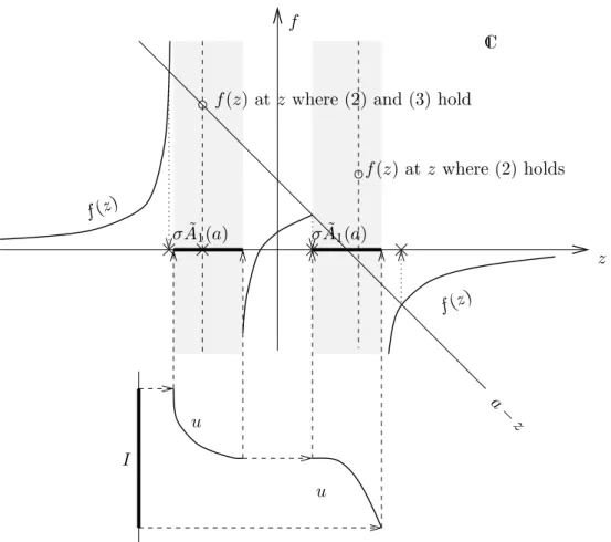
a− z f(z) at zwhere (2) holds f(z) atz where (2) and (3) hold

Figure 1: The meaning of (7): The eigenvalues of A₁(a) are represented by little crosses on the z-axis.

(11)

An easy consequence⁴ is

Proposition 1.6 Isolated real eigenvalues of A˜₁(a) vary monotonously with a.

1.2 Eigenvalues of A˜₁(a) on the border of R^µessu

The question arises what happens to formerly isolated eigenvalues when a moves into Rµessu.

Let us consider the eigenvaluez₋(a)< minR^µessufirst, if aincreases. The situation for z₊ and decreasing a is the same. Other eigenvalues outside Rµessu, behave similar (see Remark 1.7), but also those eigenvalues inside Rµessu, which can move in an interval (u₋, u₊), for which v u⁻¹((u₋, u₊))={0}. The latter is plausible since the operatory7→u·y can be decomposed into two parts then which act on orthogonal subspaces ofL²µ, one includingv. So the extension A˜₁(a) leaves one of these two operators unperturbed, and the other has no spectrum in (u₋, u₊).

Proposition 1.7 Set

a₋= minRµessu+ Z

I

|v|²

u−minR^µessudµ∈IR∪{+∞}.

Then A˜1(a) has one eigenvalue z₋(a) < Rµessu for a < a₋ and none for a > a₋. Further it holds

alimրa−

z₋(a) = minRµessu. (8)

If a₋∈IR, this means that the eigenvalue z₋(a) has joinedRµessu ifa > a₋. Proof: By the Fatou-Lemma,

a₋= lim

zրminR^µessu(z+f(z)). (9)

Hence,a₋∈IR implies that (7) cannot be fulfilled by a numberz≤minR^µessu if a > a₋. Equation (8) is a consequence of z 7→ z+f(z) being continuous, strictly monotonous, and

thus bijective, together with (9). ♥

Remark 1.6 Note thatvmay vanish on some sets of positiveµ-measure. Then Proposition 1.7 may hold trivially. For instance, ifv(u⁻¹((−∞, u₊))) ={0}, and minRµessu < u₊, the function z₋ is even analytic fora neara₋ sincez < u₊ stays true there. See the notes at the beginning of this section.

Proposition 1.8 Let a₋ of Proposition 1.7 be finite and µ(v⁻¹({0})) = 0. Then the following are equivalent:

(i) minRµessu is an eigenvalue of A˜₁(a₋).

4This could be seen as well from the monotony ofz7→z−a+f(z).

(12)

(ii) ^dz⁻_da^(a)(a) remains bounded foraրa₋.

Proof: Property (i) via Proposition 1.1 implies (2) which is equivalent to (ii) by Proposition 1.5 via Fatou-Lemma.

On the other hand, for a=a₋ (3) always holds if the integral converges. This convergence is implied by (ii), which is a consequence of (2) via Fatou-Lemma again. Hence (ii) also implies

(i). ♥

Remark 1.7 Statements similar to Propositions 1.8 and 1.7 can be proved for all pointsz_∂ on the border of Rµessu in quite the same manner. Then the values a₋ have to be substituted by by z∂ +^R_I _u^|₋^v^|_z²

∂dµ ∈ {−∞} ∪IR∪{+∞}. Moreover, before the Fatou-Lemma can be applied, some integrals have to be split into two parts in order to get purely positive and purely negative integrands.

1.3 Eigenvalues of A˜₁(a) in R^µessu

We continue the study of the operators ˜A₁(a) of the previous section. In this section, we restrict ourselves to the Lebesgue measure µ(t) = t on I and assume I to be an interval. These assumptions implyR^µessu=u(I) if u is continuous.

Proposition 1.9 Let I be an interval and µ(t) = t determine the Lebesgue-measure on I.

Further assume u to be differentiable and v to be continuous.

Then

v(u⁻¹({z})) ={0} if z is an eigenvalue of A˜₁(a) for which (2–3) hold.

Proof: Choose t_z ∈ u⁻¹({z})∩I. Then there is a number ε₀ > 0 such that (t_z−ε₀, t_z] ⊆ I or [tz, tz+ε₀) ⊂ I. Without loss of generaltiy we assume the latter case. The former can be explored analogously.

Since u is differentiable at tz, we can estimate

|u(t)−z| ≤(1 +|u^′(tz)|)|t−tz| (10) fort∈I sufficiently neart_z.

Assume v(tz)6= 0. Then continuity of v tells us

|v(t)| ≥ |v(tz)|

2 >0 (11)

fort∈I sufficiently neartz.

Now use (10) and (11) in condition (2). For sufficiently smallε >0 this yields:

Z

I

|v|²

|u−z|²dt ≥ |v(tz)|² 4(1 +|u^′(t_z)|)²

Z tz+ε tz

|t−tz|⁻²dt= +∞.

(13)

Hence, (2) is not fulfilled. This contradicts the converse assumption. Consequently v(tz) = 0.

♥

Remark 1.8 Note that the arguments in the proof of Proposition 1.9 can be used to show that not only (2) is violated if v(tz)6= 0, but f(z) does not exist either. This follows from (10) and (11) by

Z

I

|v|²

|u−z|dt ≥ |v(tz)|² 4(1 +|u^′(tz)|)

Z _t_z_+ε

tz

|t−tz|⁻¹dt= +∞.

Remark 1.9 Remembering the proof of Proposition 2.7, you see that line (5) states that the measure µof the setv⁻¹(C\{0})∩u⁻¹({z}) is zero in the case c6= 0. This case is just the case when (2–3) are valid. Proposition 1.9 strengthens this by asserting that that set is empty in fact, under additional assumptions onI,µ,u, and v.

The following is an immediate consequence of Proposition 1.9.

Proposition 1.10 Under the assumptions of Proposition 1.9 it holds: If v⁻¹({0})is finite, then there are only finitely many pairs (a, z) such that (2–3) hold.

From Proposition 1.10 can be seen that eigenvalues inR^µessuare not stable in general. If (4) is not valid, we can even prove instability from suitable conditions. Under such conditions, those eigenvalues must disappear leaving no trace in σpA˜1(a) when ais changed.

The assumption that v(t) = 0 only at finitely many t ∈ I is important here. This will be illustrated by Proposition 1.12, which uses some preliminaries.

Proposition 1.11 For all sequences (ak)_k_∈ZZ of real numbers, there is a nonnegative, bounded functionv∈C^∞((−1,+1)) such that

v⁻¹({0})∩(−1,+1) ={tanhk:k∈ZZ}, (12) and for all k∈ZZ

Z ₁

−1

|v(t)|²

|t−tanhk|²dt <∞ (13)

and Z ₁

−1

|v(t)|²

t−tanhkdt=ak (14)

hold.

Proof: Note at the beginning: Exceptionally, throughout this proof we consider all linear spaces as linear spaces over the field IR of real numbers! Especially the spaces of sequences are supposed to contain real-valued sequences only.

(14)

Let us remember the familiar C^∞(IR) testing functionϕ(t) = (

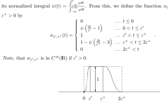
e⁻^1−t¹² . . . −1< t <1 0 . . . else and its normalized integral ψ(t) =

Rt

−∞ϕdt

R+∞

−∞ϕdt. From this, we define the function w_ε′,ε⁺ for 0 ≤ ε^′ ≤ ε⁺ >0 by

w_ε′,ε⁺(t) =











0 . . . t≤0

ψ^2t_ε′ −1 . . . 0< t≤ε^′ 1 . . . ε^′ < t≤ε⁺ 1−ψ_ε^2t+ −3 . . . ε⁺ < t≤2ε⁺ 0 . . . 2ε⁺< t

.

Note, thatw_ε^′_,ε⁺ is in C^∞(IR) if ε^′ >0.

0 ε^′ ε⁺ 2ε⁺

? 6 1

Figure 2: The functionw_ε′,ε⁺, sketched.

We define tk = tanhk. Additionally we shall make use of a sequence of positive numbers bk

fulfilling

+X∞ k=−∞

b_k=ε <

R₂

0 ψ(t−1)

t dt

2 . (15)

Then there is a sequence of positive numbers

ε⁺_k < min(t_k+1−tk, tk−tk−1)

4 (16)

such that

Z t_k+1 t_k−1

w_ε′

k,ε⁺_k(t−tk) +w_ε′

k,ε⁺_k(tk−t)

|t−t_k₋₁|² dt ≤ b_k, (17) Z t_k+1

t_k−1

w_ε′

k,ε⁺_k(t−tk) +w_ε′

k,ε⁺_k(tk−t)

|t−t_k+1|² dt ≤ b_k. (18) Let a sequence (a^′_k)_k_∈ZZ be given.⁵ Then there is a sequence of positive numbersε^′_k such that

|a^′_k| ≤ Z _t_k+1

t_k−1

w_ε′

k,ε⁺_k(t−tk) t−tk

dt. (19)

5This will be the sum of the sequence (ak)_k∈ZZ and a second, fix sequence (a⊥k)_k∈ZZ.

(15)

For brevity, let us set g_k⁺(t) =w_ε′

k,ε⁺_k(t−tk) andg_k⁻(t) =w_ε′

k,ε⁺_k(tk−t). Note that (16) implies suppg_k⁺⊂

t_k,t_k+t_k+1 2

, suppg_k⁻⊂

t_k+t_k₋₁ 2 , t_k

. (20)

For any bounded (real valued) sequence h = (hk)_k_∈ZZ we define the nonnegative function g by

gh(t) =

+∞

X

k=−∞

|h_k|+h_k

2 g⁺_k(t) + |h_k| −h_k 2 g_k⁻(t)

. (21)

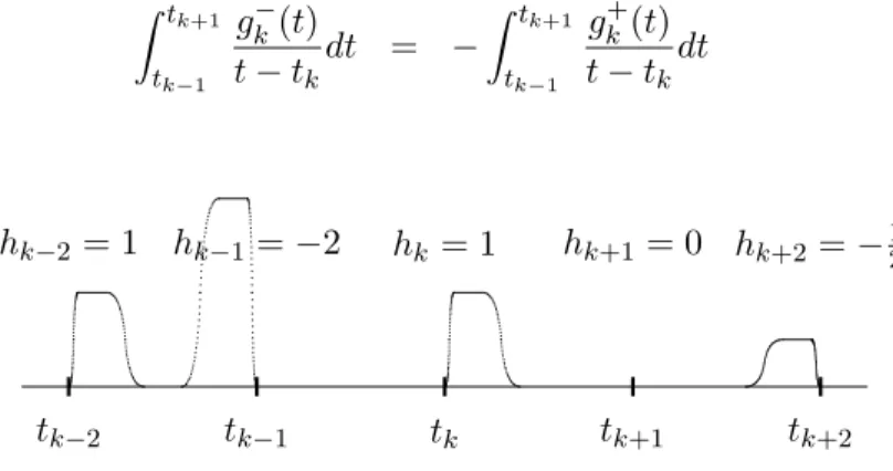
This may seem a bit queer, but it is necessary to decompose (h_k)_k_∈ZZ according to the sign of its elements, since our aim is something similar tov=√gh. Hence,ghmust be nonnegative and the signs of the numbershkmust be encoded nonlinearly by the distinction between g_k⁺ andg_k⁻. See Figure 3. Note at this point thatg_k⁻(t−t_k) =g⁺(t_k−t) and thus

Z _t_k+1

t_k−1

g_k⁻(t) t−tk

dt = − Z _t_k+1

t_k−1

g_k⁺(t) t−tk

dt hold.

tk−2 tk−1 t_k t_k+1 t_k+2 hk−2 = 1 hk−1 =−2 h_k= 1 h_k+1= 0 h_k+2 =−¹₂

Figure 3: The shape of a typical functiong_h, sketched.

From (20) follows that in the sum (21) for every t maximally onek yields a nonzero contri- bution to the sum. Consequently, g_h ∈C^∞(I). Moreover, g_h is bounded bykhk_∞, because the functions g_k⁺ and g_k⁻ are bounded by 1, and only one of g⁺_k(t) and g⁻_k(t) may be nonzero for each specific numbert.

So far we have defined a functiongh from a sequenceh. Now from this, define two sequences T h and Ihsetting

(T h)_k = Z ₊₁

−1

g_h(t)

t−t_kdt (22)

and

(Ih)_k=

Z ^tk⁺^tk+1₂

tk−1+tk 2

g_h(t) t−t_kdt=

Z +1

−1

|hk|+hk

2 g⁺_k(t) +^|^h^k^|−₂^h^kg_k⁻(t)

t−t_k dt=h_k Z +1

−1

g_k⁺(t)

t−t_kdt. (23) Obviously, the integral in (23) converges, because g_k⁺ is a bounded differentiable function with g⁺_k(tk) = 0. Therefore we know

|g_k⁺(t)|=O(t−tk). (24)

(16)

(Compare the argumentation of Proposition 1.14). Ifhis a bounded sequence, then the integral (22) converges as well for the same reason.

In this way, two operators T and I have been defined on ℓ^∞IR. The operatorI is linear, the operatorT is not linear but stands in an almost linear relation toI, see (26). So it will turn out to be almost linear itself (see (30) in footnote 7).

But first, let us show that I is invertible on the space IRZZ of all real-valued sequences. This follows from (23) and that

Z +1

−1

g⁺_k(t) t−t_kdt =

Z 2ε⁺_k 0

g⁺_k(t) t−t_kdt≥

Z ε^′_k 0

g⁺_k(t) t−t_kdt=

Z ε^′_k 0

ψ^2(t_ε⁻′^t^k⁾

k −1

t−t_k dt

=

t^′=^2(t_ε⁻′^t^k⁾ k

dt^′=_ε²′ k

= Z ₂

0

ψ(t^′−1)

t^′ dt^′ =C_I⁻¹ >0

is bounded from zero by a positive constant. Hence, we can write for a sequence (h^′_k)_k_∈ZZ:

(I⁻¹h^′)_k = h_k R₊₁

−1 g_k⁺(t)

t−t_kdt .

As the positive constantC_I−1 does not depend onk, the operator I⁻¹ acts continuously on the space ℓ^∞IR⊂IRZZ of bounded real sequences. It holds

I⁻¹

∞≤ 1 C_I−1

. (25)

Now we return to T in order to prove: ⁶

∀h, h^′ ∈ℓ^∞IR :

T(h+h^′)−T h−Ih^′_∞≤2εh^′_∞ (26) From the basic inequality

|c±d| − |c|≤ |d| we get that for all k∈ZZ

|h_k+h^′_k|+ (h_k+h^′_k)

2 −|h_k|+h_k 2

≤ |h^′_k|,

|hk+h^′_k| −(hk+h^′_k)

2 −|hk| −hk

2

≤ |h^′_k| hold. We use this to estimate

(T(h+h^′))_k−(T h)_k−(Ih^′)_k=

Z ₊₁

−1

g_h+h^′(t)−g_h(t) t−tk

dt−(Ih^′)_k

6Note that neither of the three sequencesT(h+h^′),T h, and Ih^′ needs to be bounded, but (26) states that T(h+h^′)−T h−Ih^′ is.

(17)

=

(I(h+h^′)−Ih−Ih^′)k

| {z }

0

+ Z

(−1,+1)\

htk−1+tk

2 ,^tk⁺^tk+1₂

ig_h+h^′(t)−g_h(t) t−tk

dt

= Z

(−1,+1)\

htk−1+tk

2 ,^tk⁺^tk+1₂

i

+X∞ j=−∞

|hj+h^′_j|+(hj+h^′_j)

2 −^|^h^j^|₂^+h^j

g⁺_j (t) +

|hj+h^′_j|−(hj+h^′_j)

2 −^|^h^j^|−₂ ^h^j

g⁻_j (t) t−tk

dt

≤ Z

(−1,+1)\

h_tk−1+tk

2 ,^tk⁺^tk+1₂

i

+X∞ j=−∞

|h^′_j|g_j⁺(t) +g⁻_j (t)

|t−t_k| dt

≤2h^′

∞

Z

(−1,+1)\

htk−1+tk

2 ,^tk⁺^tk+1₂

i

+∞

X

j=−∞

g_j⁺(t) +g_j⁻(t)

|t−tk|² dt

≤2h^′

∞

X

j∈ZZ\{k}

Z ^tj⁺^tj+1

2 tj−1+tj

2

g_j⁺(t) +g_j⁻(t)

|t−tk|² dt≤2h^′

∞ +X∞ j=−∞

b_j = 2εh^′

∞. In the last line remember the definitions ofg⁺_j and g_j⁻ and (17–18). From these follows

Z ^tj⁺^tj+1

2 tj−1+tj

2

g_j⁺(t) +g⁻_j (t)

|t−tk|² dt≤bj (27) forj =k+ 1 (from (17)), and for j =k−1 (from (18)) at first. A fortiori, the inequality (27) for arbitrary j6=k follows from these two cases. Well now, so we have proved (26).

Setting h= 0 in (26), we see that

kT −Ik_∞≤2ε. (28)

Remembering (25), we can estimate

1−I⁻¹T

∞≤I⁻¹

∞kT−Ik_∞≤ 2ε C_I−1

(29) from (28). ⁷

From (26) and (29) we see

I⁻¹T(h+h^′)−I⁻¹T h

∞ ≤ 0 +I⁻¹Ih^′

∞+ 2ε C_I−1

h^′_∞=

1 + 2ε C_I−1

h^′_∞. (31) Consequently, I⁻¹T is continuous onℓ^∞IR.

7From (28), by the way, we can also get T(h+h^′)−T h−T h^′

∞≤

T(h+h^′)−T h−Ih^′

∞+kT−Ik_∞ h^′

∞≤4ε h^′

∞, (30) which states thatT is “nearly linear”.

(18)

Next we want to show thatI⁻¹T is an invertible operator onℓ^∞IR. The estimation (29) lets us think of Banach’s Fixed Point Theorem, but alas, I⁻¹T is not linear. However, a property such as (26)⁸ suffices to be able to exploit the idea of this Fixed Point Theorem if ε is sufficiently small.

Fix a sequence h⁰ ∈ℓ^∞IR. Then we set inductively hⁱ =h⁰−I⁻¹T





i−1

X

j=0

h^j



. (32)

The assertion is that for all i∈IN it holds hⁱ

∞≤ 2ε

C_I⁻¹ i

h⁰

∞. (33)

Fori= 0, this is obvious. If (33) holds fori >0, then

hⁱ⁺¹

∞ =

h⁰−I⁻¹T





i−1

X

j=0

h^j+hⁱ





∞

≤

h⁰−I⁻¹T





i−1

X

j=0

h^j



−I⁻¹Ihⁱ

∞

+ 2 ε C_I−1

hⁱ

∞= 0 + 2 ε C_I−1

hⁱ

∞

proves that it holds for i+ 1, too. Hence it is true for all i∈IN. Remember (15) to see from this that h^Σ = ^P⁺_i=0^∞hⁱ converges in ℓ^∞IR. Equation (32) together with the continuity of I⁻¹T (see (31)) tell us thatI⁻¹T h^Σ =h⁰. Hence (I⁻¹T)⁻¹=T⁻¹I exists on ℓ^∞IR.

Now we return to the initial problem to determine the function v that fulfills (13–14) for the sequence (ak)_k_∈ZZ given. Set

g_⊥(t) =

( ϕ^2t_t⁻^t^k⁻^t^k+1

k+1−tk

. . . t∈(tk, t_k+1) for some k∈ZZ 0 . . . else.

This defines a positive bounded function g_⊥ ∈ C^∞((−1,1)) such that g_⊥⁻¹({0})∩(−1,1) = {tk:k∈ZZ}. We use this function in order to assure (12). Obviously, the integrals

a_⊥_k= Z +1

−1

g_⊥(t)

t−t_kdt (34)

converge because of the same reasons that assured the convergence of (23), see (24).

With this sequence (a_⊥_k)_k_∈ZZ, we set a^′_k = ak−a_⊥_k and construct the operator T⁻¹I ac- cordingly. From (19) we see that in any case I⁻¹a^′∈ℓ^∞IR. Thus we can define the sequence

h=T⁻¹II⁻¹a^′ ∈ℓ^∞IR. With this sequence, we setg=g_⊥+gh and

v=√g.

8Property (30) would do as well.

(19)

Note here thatg_⊥≥0 andgh ≥0, and that both functions are bounded.

First, it is to show that v ∈ C^∞((−1,+1)) holds. From g_⊥ ∈C^∞ and gh ∈ C^∞ it is clear that v is infinitely differentiable at pointst∈(−1,+1) whereg(t) =g_⊥(t) +g_h(t)>0. That is why we only have to consider those t ∈(−1,+1) where both of these functions vanish. These are exactly the pointstk fork∈ZZ.

Near the pointstk,gcan be written as a nonnegative linear combination of the four functions t 7→ ϕ^2t⁻_t^t^k−1⁻^t^k

k−t_k−1

, t 7→ ϕ^2t⁻_t^t^k⁻^t^k+1

k+1−t_k

, t 7→ ψ^2(t_ε⁻′^t^k⁾

k −1, and t 7→ ψ^2(t_ε^k′⁻^t)

k −1. The squareroot of such a linear combination is aC^∞-function aroundtk.

The argument (see (24)) that showed the convergence of the integrals (23) and (34) above, can be modified: Because ofg∈C^∞(I) and g(tk) =g^′(tk) = 0, we knowg(t) =O(|t−tk|²) for tneart_k. Moreover, gis bounded on I. This yields (13). As a consequence of (13), the integral in (14) converges, too.

It remains to show (14) at last. But this is evident from Z ₊₁

−1

|v(t)|² t−tk

dt = Z ₊₁

−1

g_⊥(t) +gh(t) t−tk

dt=a_⊥_k+ (T h)k =a_⊥_k+ (T T⁻¹II⁻¹a^′)k=ak.

♥

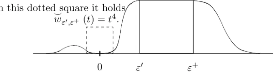
Remark 1.10 It is in no way necessary to choose the essential singularities of the function g exactly at the valuest_k. A type of functions^⌣w_ε′,ε⁺, similar to the functionsw_ε′,ε⁺, but equal to t⁴ in a small neighbourhood of 0 will do as well, see Figure 4.

0 ε^′ ε⁺

In this dotted square it holds_⌣ w_ε′,ε⁺ (t) =t⁴.

Figure 4: A suggested function ^⌣w_ε′,ε⁺, sketched.

From Proposition1.11 follows

Proposition 1.12 There is a function v∈C^∞((−1,+1)) such that A˜₁(a) = a v^∗

v y7→(t7→t·y(t))

!

has infinitely many eigenvalues in(−1,+1) for each a∈Q.

Proof: Enumerate Q×IN by numbers k∈ZZ. Then take the first componentqkof the elements (qk, nk) of this sequence. This yields an enumeration of Q, where each number is attained infinitely often.