An optical readout for the LISA gravitational reference sensor

(1)

An Optical Readout for the

LISA Gravitational Reference Sensor

D I S S E R T A T I O N

zur Erlangung des akademischen Grades Dr. rer. nat

im Fach Physik eingereicht an der

Mathematisch-Naturwissenschaftlichen Fakultät I Humboldt-Universität zu Berlin

von

Dipl. Phys. Thilo Schuldt geboren am 19.04.1975 in Singen

Präsident der Humboldt-Universität zu Berlin:

Prof. Dr. Dr. h.c. Christoph Markschies

Dekan der Mathematisch-Naturwissenschaftlichen Fakultät I:

Prof. Dr. Lutz-Helmut Schön Gutachter:

1. Prof. Achim Peters, Ph.D.

2. Prof. Dr. Claus Braxmaier 3. PD Dr. Hans-Jürgen Wünsche eingereicht am: 15.10.2009

Tag der mündlichen Prüfung: 14.07.2010

(2)

Abstract

The space-based gravitational wave detector LISA (Laser Interferometer Space Antenna) consists of three identical satellites. Each satellite accommo- dates two free-flying proof masses whose distance and tilt with respect to its corresponding optical bench must be measured with at least 1 pm/√

Hz sensitivity in translation and at least 10 nrad/√

Hz sensitivity in tilt measurement.

In this thesis, a compact optical readout system – consisting of an op- tomechatronic setup together with associated electronics, data acquisition and software – is presented, which serves as a prototype for the LISA proof mass attitude metrology. We developed a polarizing heterodyne interferometer with spatially separated frequencies. For optimum common mode rejection, it is based on a highly symmetric design, where measurement and reference beam have the same frequency and polarization, and similar optical pathlengths.

The method of differential wavefront sensing (DWS) is utilized for the tilt measurement. An intrinsically highly stable Nd:YAG laser at a wavelength of 1064 nm is used as light source; the heterodyne frequencies are generated by use of two acousto-optic modulators (AOMs).

In a first prototype setup noise levels below 100 pm/√

Hz in translation and below 100 nrad/√

Hz in tilt measurement (both for frequencies above 10⁻¹Hz) are achieved. A second prototype was developed with additional intensity stabilization and phaselock of the two heterodyne frequencies. The analog phase measurement is replaced by a digital one, based on a Field Programmable Gate Array (FPGA). With this setup, noise levels below 5 pm/√

Hz in translation measurement and below 10 nrad/√

Hz in tilt measurement, both for frequencies above 10⁻²Hz, are demonstrated. A noise analysis was carried out and the nonlinearities of the interferometer were measured.

The interferometer was developed for the LISA mission, but it also finds its application in characterizing the dimensional stability of ultra-stable materials such as carbon-fiber reinforced plastic (CFRP) and in optical profilometry.

The adaptation of the interferometer and first results in both applications are presented in this work. DBR (Distributed Bragg-Reflector) laser diodes represent a promising alternative laser source. In a first test, laser diodes of this type with a wavelength near 1064 nm are characterized with respect to their spectral properties and are used as light source in the profilometer setup.

(3)

Zusammenfassung

Der weltraumgestützte Gravitationswellendetektor LISA (Laser Interfero- meter Space Antenna) besteht aus drei identischen Satelliten, an Bord derer sich jeweils zwei frei schwebende Testmassen befinden. Die Lage der einzel- nen Testmassen in Bezug auf die zugehörige optische Bank muss mit einer Genauigkeit besser 1 pm/√

Hz in der Abstands- und besser 10 nrad/√ Hz in der Winkelmessung erfolgen.

In der vorliegenden Arbeit wird ein kompaktes optisches Auslesesystem – bestehend aus einem optomechanischen Aufbau mit zugehöriger Elektro- nik, Datenerfassung und Software – präsentiert, welches als Prototyp für die- se Abstands- und Winkelmetrologie dient. Das dafür entwickelte polarisie- rende Heterodyn-Interferometer mit räumlich getrennten Frequenzen basiert auf einem hoch-symmetrischen Design, bei dem zur optimalen Gleichtakt- Unterdrückung Mess- und Referenzarm die gleiche Polarisation und Frequenz sowie annähernd gleiche optische Pfade haben. Für die Winkelmessung wird die Methode der differentiellen Wellenfrontmessung (differential wavefront sensing, DWS) eingesetzt. Als Lichtquelle wird ein Nd:YAG Festkörper-Laser bei einer Wellenlänge von 1064 nm verwendet; die Heterodyn-Frequenzen werden mittels zweier akusto-optischer Modulatoren (AOMs) generiert.

In einem ersten Prototyp-Aufbau wird ein Rauschniveau von weniger als 100 pm/√

Hz in der Translations- und von weniger als 100 nrad/√

Hz in der Winkelmessung (beides für Frequenzen oberhalb 10⁻¹Hz) demonstriert. In einem zweiten Prototyp-Aufbau werden zusätzlich eine Intensitätsstabilisierung und ein Phasenlock der beiden Frequenzen implementiert. Die analoge Pha- senmessung ist durch eine digitale, auf einem Field Programmable Gate Ar- ray (FPGA) basierende, ersetzt. Mit diesem Aufbau wird ein Rauschen kleiner 5 pm/√

Hz in der Translationsmessung und kleiner 10 nrad/√

Hz in der Win- kelmessung, beides für Frequenzen größer 10⁻²Hz, erreicht. Eine Rausch- Analyse wurde durchgeführt und die Nichtlinearitäten des Interferometers be- stimmt.

Das Interferometer wurde im Hinblick auf die LISA Mission entwickelt, findet seine Anwendung aber auch bei der Charakterisierung der dimensio- nalen Stabilität von ultra-stabilen Materialien wie Kohlefaser-Verbundwerk- stoffen (carbon-fiber reinforced plastic, CFRP) sowie in der optischen Pro- filometrie. Die Adaptierung des Interferometers dazu sowie erste Resultate zu beiden Anwendungen werden in dieser Arbeit präsentiert. Eine alternative Laserquelle stellen DBR (Distributed Bragg-Reflector) Laserdioden dar. In einem ersten Test werden Laserdioden dieses Typs mit einer Wellenlänge na- he 1064 nm hinsichtlich ihrer spektralen Eigenschaften charakterisiert und im Profilometer als Lichtquelle eingesetzt.

(4)

(5)

Introduction

The history of astronomy is the history of receding horizons.

Edwin Hubble Since the beginning of mankind people looked into the sky, and tried to under- stand the presence and the motions of the luminaries. Outer space implicated key human questions such as the existence of god, the creation of the universe and the Earth and the possibility of extraterrestrial life. Not only was all instrumentation available at that time used in order to get a deeper understanding of astronomy and astrophysics, but humankind’s ambition to explore the sky and the universe was one of the main technology drivers throughout history.

First observations were made by naked eye, but the invention of the telescope at the beginning of the 17th century, and the knowledge of its potential by Galileo Galilei, enabled much more detailed observations and motivated modern astronomy.

The optical setup, the optical component fabrication and the resulting telescope resolution were improved in the following enabling an in-depth analysis of celestial bodies in the visible wavelength region.

With the discovery of infrared radiation by the astronomer William Herschel in 1800, it became clear that the visible wavelength region is only a detail of a much more general spectrum which could be mathematically described by Maxwell’s electromagnetic theory of light in 1864. The electromagnetic wave spectrum spans the whole wavelength region, including radio waves (λ > 1 m), microwaves (λ = 1 m. . .1 mm), infrared (λ =1 mm. . .700 nm), visible (λ =750. . .380 nm), ultra- violet (λ =400. . .1 nm), X-rays (λ =10. . .0.01 nm) and gamma radiation (λ <

10 pm). Detecting light from outer space means building specific detectors for each wavelength region and to combine the information obtained in order to get a more extensive knowledge of astrophysical processes.

The Earth’s atmosphere is a strong limitation for outer space observation. First because the telescope’s angular resolution is limited by turbulence in the atmosphere, and second because the atmosphere has strong absorptions in the electromagnetic spectrum. The atmosphere blocks high energy radiation such as X- rays, gamma and ultra-violet radiation and shows strong absorption lines in the infrared. When it became possible to launch artificial satellites into an orbit out- side the Earth’s atmosphere, space-based telescopes were developed, launched and

(10)

2 Introduction operated. Examples are the radio astronomy satellite HALCA, the Hubble space telescope in the visible, near-ultra-violet and near-infrared spectral ranges, the Her- schel telescope in the far infrared spectral range, the Extreme Ultra-violet Explorer (EUVE), the X-ray observatory XMM-Newton, the Compton Gamma Ray Observa- tory (CGRO) and COBE, a satellite investigating the cosmic microwave background radiation.

Up until now, telescopes detecting all parts of the electromagnetic spectrum – covering a range of 20 orders of magnitude in frequency – are operating. Each time the bandwidth was expanded to a different wavelength region in the electromagnetic spectrum, a different aspect of the universe was observed. But still, essentially all our knowledge about outer space is based on observations of electromagnetic waves emitted by individual electrons, atoms and molecules¹. When Einstein published his Theory of General Relativity in 1915, a new kind of waves was predicted:

gravitational waves caused by asymmetrically accelerated masses. In contrast to electromagnetic waves, which are easily scattered, absorbed and dispersed, gravitational waves travel nearly undisturbed through space and time – opening a com- pletely new access to space observation.

Gravitational waves distort spacetime, and therefore change the distances between free macroscopic bodies. As their amplitude is tiny, only processes involving huge masses can produce significant and measurable signals. Sources of gravitational waves cover a frequency range from 10⁻¹⁶Hz to 10⁴Hz, and include galactic binary systems (such as neutron star binaries, black hole binaries, white dwarf binaries), mergers of massive black holes and supernovae collapses. While the high- frequency range 10 to 10³Hz can be covered by ground-based detectors, the low frequency range below 0.1 Hz is only accessible by space-based detectors.

Several ground-based gravitational wave detectors already exist and are on the way to achieve their designated sensitivities. Space-based detectors are proposed and studies on their design are beeing carried out. One specific space mission is LISA (Laser Interferometer Space Antenna) – an ESA/NASA collaborative space mission dedicated to the detection of gravitational waves in the low-frequency range 30µHz to 1 Hz. Three similar satellites form a giant Michelson interferometer in space with an armlength of 5 million kilometers as shown in Fig. 1. The LISA mission, planned to be launched around 2019, is currently in the so-called mission formulation phase, where the science requirements are fixed and the mission requirements are assigned. The corresponding study is carried out at Astrium GmbH – Satellites, Friedrichshafen, on behalf of ESA. This study also reveals critical subsystems and drives their technology demonstration first in on-ground laboratory experiments.

One of the subsystems is the readout of the LISA gravitational reference sensor

1Also the analysis of meteorites and the detection of neutrinos are used for the study of astrophysical processes.

(11)

Introduction 3

Figure 1.: Artist’s view of the LISA space mission. Three satellites form a Michel- son interferometer with an armlength of∼5 million kilometers (source:

Astrium GmbH).

(GRS) where the position and tilt of a free flying proof mass with respect to the optical bench must be measured with pm-sensitivity in translation and nanoradian- sensitivity in tilt measurement. The needed sensitivity requires for an optical readout (ORO) where different implementations are conceivable. Several groups around the world are investigating different approaches, where interferometric measurements, which can be realized in a variety of designs, offer the highest potential.

They can be subdivided in polarizing or non-polarizing setups, homodyne or heterodyne detection, Michelson or Mach-Zehnder type interferometers. All methods have their specific advantages and disadvantages. While an optical lever sensor is developed at the University of Napoli, interferometric methods are investigated at Stanford University (grating interferometer), University of Birmingham (homodyne polarizing interferometer; Michelson type) and Albert-Einstein-Institute Han- nover (in collaboration with University of Glasgow and Astrium GmbH – Satellites, Friedrichshafen; heterodyne non-polarizing interferometer, Mach-Zehnder type).

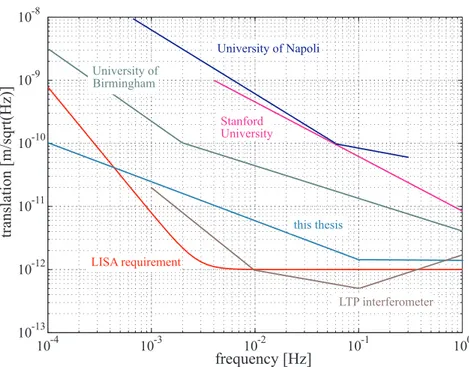
The currently achieved noise levels of the different ORO implementations are shown in Fig. 2, together with the LISA science requirements. The readout systems developed by the Universities of Napoli, Birmingham and Standford can currently not demonstrate the noise levels required for LISA. The LTP interferometer – specifically built with respect to the LISA Pathfinder mission requirements – uses a glass ceramics baseplate where the optical components are fixed to using hydroxide-catalysis bonding technology. An alternative ORO implementation for LISA – based on single-path polarizing heterodyne interferometry – will be dis-

(12)

4 Introduction

10^-4 10^-3 10^-2 10^-1 10⁰

10^-13 10^-12 10^-11 10^-10 10^-9 10^-8

frequency [Hz]

translation [m/sqrt(Hz)]

LISA requirement

LTP interferometer this thesis

University of Birmingham

University of Napoli

Stanford University

Figure 2.: Achieved noise levels of different optical readout implementations. Also included is the LISA science requirement.

cussed in the following and is the subject of this thesis. It is built as a laboratory setup, using a cast aluminum baseplate and optical mounts made of aluminum and stainless steel. The achieved noise levels are also included in Fig. 2.

Outline of the thesis: A short introduction to the physics of gravitational waves is given in Chapter 1 which also includes an overview of different methods for gravitational wave detection. A detailed outline of the LISA space mission is given in Chapter 2, focussing on the optical setup. Different possibilities for the optical readout of the LISA gravitational reference sensor are outlined in Chapter 3 where Chapter 4 will focus on interferometric concepts. Our interferometer design is presented in Chapter 5 and Chapter 6 where the experimental setups and measurements are shown. First applications of the interferometer in high-accuracy dilatometry and optical profilometry are presented in Chapter 7. Chapter 8 comprises a conclusion and the next steps with respect to an enhanced interferometer setup.

(13)

1. Gravitational Waves and Their Detection

Gravitational waves are deduced from the field equations in Einstein’s theory of general relativity which was first published in 1915. Although most parts of the theory of general relativity are experimentally verified to a very high degree of precision, up until now, there has been no direct verification of the existence of gravitational waves.

This chapter shortly describes how gravitational waves result from general relativity, what kind of astrophysical events cause such waves and what different techniques of gravitational wave detection exist.

1.1. General Relativity

The theory of general relativity presents the relativistic generalization of New- ton’s gravitational theory where gravity can be expressed as a spacetime curvature (cf. e.g. [1, 2]). The Einstein field equations describe the relation between the Einstein tensor G_{µ ν} representing the curvature of spacetime and the stress-energy tensorT_{µ ν} which represents the mass and energy content of spacetime:

G_{µ ν} = 8πG

c⁴ T_{µ ν}. (1.1)

Here,Gis the gravitational constant andcthe speed of light. The tensorsG_{µ ν}and T_{µ ν} are symmetric; equation (1.1) therefore corresponds to a system of 10 nonlinear partial differential equations. The field equations have the same form as an elasticity equation where spacetime represents the elastic medium. It is extremely stiff as its elasticity module is given byG/c⁴≈10⁻⁴³N⁻¹.

The (infinitesimal) distancedsbetween two points in spacetime with coordinates x^µ andx^µ+dx^µ is given by

ds²=g_{µ ν}dx^µdx^ν, (1.2)

whereg_{µ ν} is the symmetric metric tensor which contains the information on spacetime curvature. In case of the flat spacetime of special relativity, the metric tensor

(14)

6 Gravitational Waves and Their Detection is given by the Minkowskian metricη_{µ ν}=diag(1,−1,−1,−1), where the distance is given by

ds²=η_{µ ν}dx^µdx^ν =−c²dt²+dx²+dy²+dz². (1.3) The Minkowskian metric is a solution of the Einstein field equations withT_{µ ν} = 0. In a weak field approximation, the metric tensor can be written as

g_{µ ν} =η_{µ ν}+h_{µ ν}, (1.4)

whereh_{µ ν}1 is a small perturbation of the Minkowskian metric and a measure of spacetime curvature. The linearized field equation is then given by

−1 c²

δ² δt²+∆

h_{µ ν} =−16πG

c⁴ T_{µ ν}. (1.5)

For a source-free space withT_{µ ν} =0, this results in a homogeneous wave equation

−1 c²

δ² δt²+∆

h_{µ ν}=0, (1.6)

with plane waves as a solution. These gravitational waves propagate with the speed of lightv=cin the direction of~k(k=ω/c):

h_{µ ν}(~r,t) =h⁰_{µ ν}sin(~k~r−ωt+φ_{µ ν}). (1.7) Two polarizations of such gravitational waves exist; they are called ‘+’ and ‘×’

and are orthogonal to one another. The gravitational wave amplitude tensorh_{µ ν} is given by

h_{µ ν} =







0 0 0 0

0 h₊ h_× 0 0 h_× −h₊ 0

0 0 0 0







. (1.8)

This means, h_{µ ν} can be described as a superposition of two gravitational waves with different polarization. Their corresponding amplitudes are given by h₊ and h_×, respectively.

Analogous to electromagnetic waves which interact with charged particles, gravitational waves interact with massive particles. For two masses separated by~L, the change in their separationδ~Lis given by (see e.g. [2])

δL L = 1

2h. (1.9)

Therefore, a gravitational wave with amplitudeh(eitherh₊ orh_×) stretches and

(15)

1.2 Sources of Gravitational Waves 7

Figure 1.1.: Illustration of the two existing polarizations ‘+’ and ‘×’ of gravitational waves and their effect on a ring of free particles [3]. The polarizations are transverse to the direction of the wave.

shrinks the distance between two free bodies. This equation also states, that gravitational wave detectors should have a large baselineLsince the change in distance δLcaused by the gravitational wave with an amplitudehincreases proportional to L.

Gravitational waves are transverse, i.e. they act in a plane perpendicular to their direction of propagation. In the transverse plane, gravitational waves are area pre- serving: when observing a ring of free particles, it will be stretched in one given direction and simultaneously squeezed in the direction perpendicular to that direction. In Fig. 1.1 the two polarizations of gravitational waves and their effect on a ring of free particles are shown schematically.

1.2. Sources of Gravitational Waves

Gravitational waves are caused by asymmetrically accelerated masses. As an exam- ple for a gravitational wave source, the amplitudehof a gravitational wave caused by a binary system where all mass is part of an asymmetric motion, is given by [3]:

h=1.5×10⁻²¹ f

10⁻³Hz

2/3 r 1 kpc

−1M M

5/3

(1.10) where f is the gravitational wave frequency (and corresponds to twice the binary orbital frequency), r is the distance source to detector andM the ‘chirp mass’ of

(16)

8 Gravitational Waves and Their Detection

Figure 1.2.: Spectrum of gravitational waves. Shown are relevant sources for the spaceborne gravitational wave detector LISA and the Earth-bound gravitational wave detector (advanced) LIGO [8].

two stellar massesM₁andM₂:

M = (M₁M₂)^3/5

(M₁+M₂)^1/5. (1.11)

Equation (1.10) also shows the order of magnitude of the gravitational wave amplitudeh. Only huge masses, which can only be found in astrophysics, can produce significant and measurable gravitational wave signals.

Sources of gravitational waves can be subdivided into three classes: bursts, periodic waves and stochastic waves – covering a frequency range from 10⁻¹⁶Hz to 10⁴Hz. Burst sources include star collapses as supernova explosions, coalescent binary systems and the fall of stars or small black holes into a supermassive black hole (M>10⁵M). Bursts only last for a very short time, i.e. a few cycles. Periodic sources with significant emission of gravitational wave radiation are double star binary systems and spinning stars as pulsars. A potential stochastic source of gravitational waves is the random primordial cosmological background¹(cf. e.g. [4]).

An overview of different sources in the frequency range 10⁻⁴Hz to 10⁴Hz is given in Fig. 1.2. An outline of gravitational wave sources and their astrophysical interest can be found e. g. in [5, 6, 7, 8].

1The cosmic gravitational wave background (CGWB) is similar to the cosmic microwave background (CMB). While the CMB dates from about 380000 years after the big bang the predicted CGWB sets in nearly instantly after the big bang.

(17)

1.3 Gravitational Wave Detection 9

1.3. Gravitational Wave Detection

Detection of gravitational waves can be distinguished into indirect and direct methods where the direct methods can be further classified into resonant bar detection and interferometric measurements.

1.3.1. Indirect Proof

The indirect proof of the existence of gravitational waves was carried out by J.

Taylor and R. Hulse by analyzing the rotation frequency of the PSR1913+16 double pulsar which they discovered in 1974 using the 305 m Arecibo radio telescope [9].

The fast rotation of a pulsar in combination with a very strong magnetic field leads to the emission of radio waves emitted in the direction of the magnetic poles of the pulsar. If this beam happens to be aligned in a way that it hits the Earth during the pulsar rotation, it hence yields to the characteristic pulses detected on Earth. The pulse repetition rate is extremely stable and pulsars can be taken as high-precision clocks. PSR1913+16 is a binary system consisting of two stars with similar mass.

The accumulated shift of the times of periastron²is shown in Fig. 1.3. The straight line corresponds to a constant rotation period. Due to energy loss, the separation between the two stars decreases causing an increase in rotation frequency. The loss of energy can be explained by gravitational waves emitted by the binary system.

The parabolic curve shows the prediction based on general relativity and presents the first indirect proof of gravitational waves [10, 11, 12]. For their work, Hulse and Taylor were awarded the Nobel Price in physics in 1993.

1.3.2. Bar Detectors

The pioneering experimental work for the direct detection of gravitational waves was carried out by Joseph Weber in the early 1960s [13]. His idea was to use large aluminum bars with a weight of 1.5 t as resonant-mass antenna where a gravitational wave passing the detector will change the length of the aluminum bar. A gravitational wave with suitable frequency will excite a vibration of the bar – the bar then rings like a bell struck with a hammer. Weber built up a detector consisting of two aluminum cylinders located at the University of Maryland and the 1000 km distant Argonne National Laboratory near Chicago. The bars are located in a vacuum chamber, isolated against vibrations and operated at room temperature.

A piezo ceramic was used for strain measurement and a coincidence measurement between both detectors with sensitivities of h=7·10⁻¹⁷ was carried out. Reso- nant bar detectors are typically sensitive in a 1 Hz bandwith around their resonant frequency which is between 700 Hz and 1000 Hz.

2Periastron is the point in the binary system where both stars have minimum distance.

(18)

Figure 1.3.: Accumulated shift of the orbital phase of the binary system PSR1913+16. The straight line corresponds to a constant period, the parabolic curve is the prediction of general relativity. The losses are caused by gravitational radiation [12].

Later, different groups built up gravitational wave detectors based on Weber’s design. They improved the sensitivity by operating the detectors at cryogenic temperatures (liquid helium at 4 K and later at ultra-low temperatures below 100 mK) and implementing an improved vibration isolation and a resonant transducer. Sev- eral detectors are currently operated throughout the world with sensitivities between 3·10⁻¹⁹ to 7·10⁻¹⁹. An overview is given in Table 1.1.

1.3.3. Interferometric Measurements

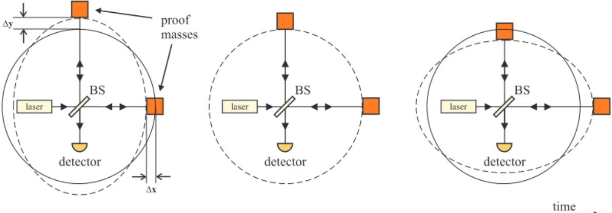
Another alternative gravitational wave detector design is using highly sensitive laser interferometry in order to measure changes in distance between widely separated proof masses. The principle of its operation is shown in Fig. 1.4 based on a Michel- son interferometer. The laser light is split at a beamsplitter, both beams are reflected at mirrored proof masses and superimposed at the initial beamsplitter. The interference of the two returned beams is detected at a photodiode. Any differential change of the distance of the proof masses – e.g. caused by a gravitational wave – causes a change in the interferometer signal. Because of their quadrupole nature, gravitational waves propagating perpendicular to the plane of the interferometer will at the same time increase the length of one interferometer arm and decrease the length of the other interferometer arm. This exactly matches the geometry of the Michelson

(19)

1.3 Gravitational Wave Detection 11

bar operating name location

material temperature reference

Allegro Baton Rouge, LA, USA Al 4 K [14]

Altair Frascati, Italy Al 2 K [15]

Auriga Lengaro, Italy Al 100 mK [7]

Explorer CERN, Switzerland Al 2.6 K [16]

Nautilus Rome, Italy Al 100 mK [17]

Niobe Perth, Australia Nb 5 K [18]

Table 1.1.: Currently operating resonant bar detectors for gravitational wave detection. The Explorer detector is operated by the same group as the Nautilus detector in Rome.

laser

proof masses

detector BS

laser

detector BS

laser

detector BS

Dy

Dx

time

Figure 1.4.: Effect of a gravitational wave on a ring of free masses. The interferometer measures the changes in distance.

interferometer.

The ideal arm length of the interferometer equals half the wavelength of the gravitational wave. For a gravitational wave with a frequency of 100 Hz this corresponds to an interferometer armlength of 1500 km. Ground-based detectors can only re- alize limited armlengths of up to several kilometers and therefore must perform a very sensitive phase measurement. Several ground-based detectors based on interferometry are on the way to achieve the designed sensitivities, an overview over current projects is given in Table 1.2. Gravitational waves with frequencies below ∼10 Hz are not accessible by ground-based detectors due to gravity gradient noise on Earth (caused e.g. by seismic activity, moving people and animals, passing clouds) [19, 20].

In order to surpass these limitations for the detection of low-frequency gravita-

(20)

name location armlength

GEO600 Hannover, Germany 600 m

LIGO (Hanford) Hanford, WA, USA 2 km and 4 km LIGO (Livingston) Livingston, LA, USA 4 km

TAMA Mitaka, Japan 300 m

VIRGO near Pisa, Italy 3 km

AIGO near Perth, Australia 80 m

Table 1.2.: Currently operated ground-based gravitational wave detectors using laser interferometry.

tional waves, space-based detectors are planned. The Laser Interferometer Space Antenna (LISA) [21, 22] has an armlength of 5 million kilometers and will detect gravitational waves in the frequency band of 30µHz to 1 Hz. The LISA mission concept will be detailed in the following chapter. A more extensive review on interferometric gravitational wave detectors can be found in [23, 24].

(21)

2. The LISA Mission Metrology Concept

First plans for a spaceborne gravitational wave detector were already proposed in the 1980s. European and American scientists both proposed space missions dedicated to the detection of gravitational waves in the low frequency band below 1 Hz utilizing high-sensitivity interferometric laser distance metrology between distant spacecraft. In 1993 the mission LISA (Laser Interferometer Space Antenna) was proposed by a team of European and US scientists to the European Space Agency (ESA) as a medium-size M3 mission candidate within ESA’s space science programme ‘Horizon 2000’. Because of the cost, LISA was later included as the third Cornerstone mission in the ESA ‘Horizon 2000 Plus’ programme and proposed to be carried out in a collaboration with the National Aeronautics and Space Ad- ministration (NASA) [21, 22]. In 1998 a LISA mission concept study [25] and a pre-phase A study [3] were performed and in the period from June 1999 to February 2000 a LISA mission concept study was carried out by Dornier Satellitensysteme GmbH (now Astrium GmbH, Friedrichshafen, Germany) [26, 27]. Since 2004 the LISA mission formulation phase study is work in progress lead by Astrium GmbH (Friedrichshafen) on behalf of ESA. During the years the mission design concept was adopted. The LISA design detailed in the following is based on the current baseline design as developed in the mission formulation phase.

2.1. Overall Mission Concept

Planned to be launched around 2019 LISA aims at detecting gravitational waves in the low frequency range 30µHz to 1 Hz. Its strain sensitivity curve is shown in Fig. 2.1 enabling the detection of gravitational waves caused e.g. by neutron star binaries, white dwarf binaries, super-massive black hole binaries and super-massive black hole formations, cf. chapter 1.2. At frequencies below 3 mHz the LISA sensitivity is limited by proof mass acceleration noise and at mid-frequencies around 3 mHz by shot noise and optical-path measurement errors. The curve rises at higher frequencies as the wavelength of the gravitational wave becomes shorter than the armlength of the LISA interferometer.

The LISA mission consists of three identical spacecraft which form an equilateral

(22)

14 The LISA Mission Metrology Concept

10^-4 10^-3 10^-2 10^-1 10⁰

10^-24 10^-23 10^-22 10^-21 10^-20 10^-19 10^-18

frequency [Hz]

GWamplitude h [dimensionless]

Figure 2.1.: LISA sensitivity curve given in the gravitational wave amplitudeh. The curve is generated by use of the LISA Sensitivity Curve Generator [28].

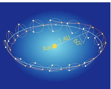
triangle in a heliocentric Earth-trailing orbit with an edge length of approx. 5 million kilometers. The formation is flying ∼20^◦ behind the Earth, corresponding to a distance of∼50 million kilometers to Earth, cf. Fig. 2.2. This orbit is a compromise between the needed electric power for data transmission to Earth, the influence of gravitational effects caused by the Earth and the need in propulsion and time for the spacecraft to reach their final position. The plane of the three spacecraft is inclined at 60^◦ with respect to the ecliptic. The triangular formation – with a nominally 60^◦ angle – is mainly maintained with a slow variation of the order of ±0.6^◦ over the annual orbit. The individual orbits of the three satellites cause the spacecraft constellation to rotate about its center one time per year.

Any combination of two arms of the LISA triangle forms a Michelson interferometer with an armlength of about 5 million kilometer. Gravitational waves passing the LISA formation will be measured as changes in the length of the interferometer arms by use of laser interferometry with ∼10 pm/√

Hz sensitivity. Each satellite contains two optical benches and two telescopes, which are orientated 60^◦ to each other and form the Y-structure of the spacecraft (cf. Fig. 2.3). The telescopes have a diameter of 40 cm and are used for sending the outgoing laser beam to the distant spacecraft as well as for collecting the incoming laser light from the distant spacecraft. A laser power of 1 W is sent to the distant spacecraft where only 150 pW are collected due to diffraction losses and the limited telescope diameter. While

(23)

2.1 Overall Mission Concept 15

60°

sun

1 A U

Figure 2.2.: The three LISA spacecraft are flying in a heliocentric orbit, 20^◦behind the Earth. (In this schematic, the LISA triangle is enlarged by a factor of 10).

in a classical Michelson interferometer, the incoming beam is reflected at the measurement mirror (and reference mirror, respectively), LISA utilizes a transponder scheme where the laser on the distant spacecraft is phase-locked to the incoming laser light and 1 W laser power is transmitted back [29]. This laser light is superimposed on the initial spacecraft with part of the original laser beam (local oscillator, LO). Due to relative velocities of the three spacecraft, the laser frequencies are Doppler shifted, resulting in a heterodyne signal on the photodiode which frequency is varying between 5 and 20 MHz over the spacecraft’s orbit. The phase measurement of this heterodyne signal gives the information about changes in length of one interferometer arm. A similar measurement is performed for each arm, where the difference between the phase measurements of two single arms yields the information about the relative change in two arms. This measurement then corresponds to the gravitational wave signal. Here, laser frequency variations would cancel in the phase measurement in case of interferometer arms exactly equal in length. Due to annual variations in the orbits of the three LISA spacecraft, laser frequency variations do not totally cancel. For frequency variation and noise suppression, additional techniques are utilized: (i) laser frequency stabilization to an optical cavity;

(ii) laser frequency stabilization to the (well defined) 5 million kilometer arm length (the so-called ‘arm locking’ [30, 31]); (iii) on-ground post-processing using ‘time

(24)

Figure 2.3.: Schematic of the LISA spacecraft. The two telescopes (movable assemblies; together with the – vertically mounted – optical bench) are oriented 60^◦to each other and point to the distant spacecraft.

delay interferometry’ [32, 33].

Two free flying proof masses on each satellite represent the end mirrors of the interferometer. Placed inside the satellite, they are shielded against external disturbances which ensures the unperturbed environment for the gravitational wave detection. Additionally, one of the proof masses acts as inertial reference for the satellite orbit (‘drag-free attitude control system’, cf. chapter 2.4). In the current baseline design, the laser light coming from the distant spacecraft is not directly reflected by the proof mass, but the (heterodyne) beat signal with the local oscillator is measured on the optical bench. In addition, the distance between optical bench and its associated proof mass has to be measured with the same accuracy as in the distant spacecraft interferometry. In this so-called strap-down architecture (cf. Fig. 2.4 and [34, 35]), the interferometric measurement of one interferometer arm is split into three technically and functionally decoupled measurements, easing the AIV (assembly, integration, verification) process:

• measurement between proof mass and optical bench on one spacecraft: d1

• measurement between two optical benches on two distant spacecraft over the distance of 5 million kilometers: d12

• measurement between optical bench and proof mass on the distant spacecraft:

d2

(25)

2.1 Overall Mission Concept 17

Figure 2.4.: Schematic of the strap-down architecture. The interferometer measuring the gravitational waves is split into three functionally decoupled interferometric measurements.

The science measurement (i.e. the interferometric measurement for detecting gravitational waves) is then given by:

d_science=d₁+d₁₂+d₂. (2.1)

The measurement of d₁ and d₂ is referred to as ‘Optical Readout (ORO)’, the measurement ofd₁₂represents the spacecraft-to-spacecraft link.

The performance requirements of the three interferometric measurements are the same and given in Table 2.1.

In order to test critical subsystems for LISA, a technology demonstration pre- cursor mission – called LISA Pathfinder – will be launched around 2010 carrying two payloads: the European ‘LISA Technology Package (LTP)’ and the Ameri- can ‘Disturbance Reduction System (DRS)’. Its main objectives are to demonstrate drag-free control of a satellite with two proof masses within an acceleration noise of 3·10⁻¹⁴

1−(f/3mHz)²

ms⁻²/√

Hz (i.e. a factor 7 less stringent than the LISA requirements), to test the feasibility of laser interferometry between two free flying proof masses with a sensitivity needed for LISA and to demonstrate the function- ality of micro-Newton thrusters in orbit [36, 37]. LISA pathfinder consists of one spacecraft with two free flying proof masses, separated by a distance of approxi- mately 30 cm.

(26)

relative displacement between

spacecraft and proof mass (sensitive axis) 1·10⁻¹² r

1+

2.8 mHz f

4

m/√ Hz dynamic range (sensitive axis) ±50µm

tilt noise (sensitive angles) 10⁻⁸ r

1+

2.8 mHz f

4

rad/√ Hz dynamic range (sensitive angles) ±100µrad

Table 2.1.: LISA requirements for the interferometric measurements as part of the strap-down architecture [26]. The sensitive axis corresponds to the line of sight of two facing telescopes on two distant spacecraft.

2.2. The LISA Optical Bench design

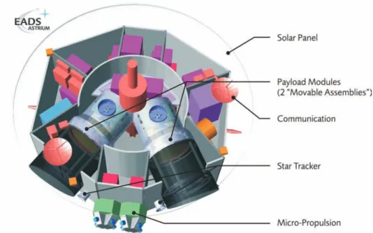
Each LISA satellite payload exists of two identical so-called ‘movable optical assemblies’, consisting of a Cassegrain telescope, an optical bench (OB) and an inertial sensor, cf. Fig. 2.5. The nominal 60^◦angle between the two assemblies can be varied by use of ultra-low-noise actuators. This is necessary due to ‘breathing’ of the LISA triangle in orbit (changing distances and angles between the spacecraft).

The cubic proof mass is made of a Au-Pt alloy with very low magnetic susceptibility and high mass. It is surrounded by the electrode housing used for electrostatic readout and actuation of the proof mass position. The housing itself is encaged by a vacuum enclosure. The Cassegrain telescope has an aperture of 400 mm and a magnification of 80. The two mirrors M1 and M2 have a distance of 450 mm where the spacer is a tube made of CFRP (carbon-fiber reinforced plastics).

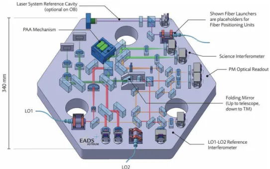
The schematic of the optical bench is shown in Fig. 2.6. It is vertically mounted behind the telescope, as seen in Fig. 2.5. Its baseplate is a 40 mm thick Zerodur hexagon, the optical components are made out of fused silica and connected to the baseplate via the method of hydroxide-catalysis bonding [38]. The optical bench will be operated at room temperature with a stability of≈10⁻⁵K/√

Hz. The fold- ing mirror in the middle of the optical bench is the interface to the telescope and to the proof mass – both optical axes coincide. Three interferometers are implemented: the optical readout of the proof mass (PM optical readout), the science interferometer (measuring changes in distance between two separated spacecraft) and the reference interferometer (measuring the phase between local oscillator LO1 and LO2 on the optical bench). All detectors are quadrant photodiodes used for differential wavefront sensing (see chapter 4.7) and also for alignment purposes.

Additionally, power monitor photodiodes and CCD cameras for acquisition of the incoming beam are placed on the optical bench.

(27)

2.3 The LISA Gravitational Reference Sensor 19

Figure 2.5.: Schematic of the LISA payload module (‘movable optical assembly’).

Shown are the telescope, the optical bench and the inertial sensor assembly.

The optical bench also includes an ultra-low-noise gimbal actuator (Point-Ahead Angle Mechanism, PAA) which corrects the angle of the incoming beam in order to achieve maximum contrast on the photodiode. The angle is varying with the annual orbit of the satellites.

The current baseline laser source is a non-planar ring-oscillator (NPRO, [39]) Nd:YAG laser at a wavelength of 1064 nm which intrinsically offers high intensity and frequency stability. The required output power is 2 W using a bulk or fiber amplifier. Each LISA satellite carries 2 phase-locked laser systems (plus 2 for re- dundancy) which are placed separately and sent to the optical bench using optical fibers.

2.3. The LISA Gravitational Reference Sensor

Each spacecraft contains two gravitational reference sensors (inertial sensors), consisting of a free flying proof mass with its housing and vacuum enclosure. Each proof mass is representing the end mirror of an interferometer arm. Also, one proof mass of each satellite is used as inertial reference for the drag-free attitude control system (DFACS, cf. chapter 2.4) of the spacecraft.

The proof mass is placed inside an electrode housing with six capacitive readouts to measure position and attitude of the proof mass. The sensor can be used in two different modes:

(28)

Figure 2.6.: Schematic of the LISA Optical Bench. (LO: local oscillator; PAA:

point ahead angle-actuator; OB: optical bench)

• The inertial reference is free flying and the the capacitive position sensors provide information of its position and attitude with respect to the sensor cage.

• The sensor can be operated as accelerometer where the proof mass is servo- controlled in such a way that it is centered inside the housing at all times. The electrostatic forces applied to the proof mass represent the satellite acceleration.

Both modes will be used during the LISA mission in order to compensate for external perturbations.

The proof mass has a dimension of 46 mm×46 mm×46 mm and is made out of a 75% Au and 25% Pt alloy because of its high density of 20 g/cm³ and its weak magnetic susceptibility. The low susceptibility minimizes effects of a variation of the magnetic environment, induced by interplanetary magnetic fields or by the magnetic field gradient caused by the satellite itself. The surface of the proof mass is coated with a thin gold layer in order to provide sufficient reflectivity for the laser interferometer. A photograph of the gravity reference sensor for LTP is shown in Fig. 2.7. The same design is intended to be used aboard the LISA satellites.

The sensor includes a capacitive readout of the proof mass position and tilt (6 DOF). The sensitive axis for the science measurement, i.e. the axis aligned with the line of sight of the telescope and therefore with the proof mass on the distant

(29)

2.4 Drag-Free Attitude Control System (DFACS) 21

Figure 2.7.: Photograph of the LTP gravitational reference sensor prototype consisting of a proof mass (left) and the corresponding electrode housing (right) [36].

spacecraft, has an additional optical link for the LISA science measurement. The sensor also includes injection electrodes for charge control of the proof mass. The emitted ultra-violet light will release photoelectrons from the proof mass surfaces.

During launch, the proof mass must be clamped. The caging mechanism must have access to the proof mass and will most probably use piezo electric actuators.

2.4. Drag-Free Attitude Control System (DFACS)

External disturbances like solar radiation pressure or solar wind will change the position of the spacecraft and thereby affect the interferometer signals caused by gravitational waves. Therefore, a free-flying proof mass inside the satellite is taken as reference for a purely gravitational orbit of the satellite. As the external disturbances only act on the surface of the satellite, the distance between the proof mass and its housing (which is rigidly connected to the satellite) is changing. In case of a drag-free controlled satellite, any change of the proof mass position is measured and the satellite is controlled in such a way that it is centered around the proof mass at any time, canceling all non-gravitational forces acting on the spacecraft (drag-free attitude control system, DFACS). The actuation of the satellite can be done e.g. by miniaturized ion engines as part of a so-calledµ-propulsion system. While external disturbances are repelled, interacting forces between the satellite and the proof mass are still present and must be controlled – in case of LISA – to a 10⁻¹⁵m/s² level. Such forces are e.g. the gravitational force caused by the satellite acting on the proof mass, and forces due to electrostatic charge of the proof mass and gradients in magnetic fields.

Drag free control of a satellite was first demonstrated in space 1972 aboard the

(30)

relative displacement between

S/C and proof mass (sensitive axis) 2.5·10⁻⁹m/√ Hz relative displacement between

S/C and proof mass (transverse axes) 10·10⁻⁹m/√ Hz absolute displacement measurement

between S/C and proof mass 5µm proof mass acceleration noise

(along the sensitive axis) 3·10⁻¹⁵ r

1+ f

8 mHz

4

m/s²/√ Hz Table 2.2.: DFACS requirements for LISA. The displacement requirements are flat

in the LISA measurement band [26].

US Navy TRIAD 1 spacecraft where the residual disturbances to the proof mass were 5·10⁻¹²g (for 3 day tracking time) [40]. Since then, the drag-free control became a standard space technology enabling several space missions with ever in- creasing sensitivity. Examples are the Earth gravity missions GRACE and GOCE and the equivalence principle test mission Gravity Probe B. DFACS will also be implemented aboard LISA Pathfinder.

In case of LISA, the proof mass is a 46 mm cube¹. It is surrounded by a housing which includes all electrodes needed for a capacitive position readout, which is current baseline for LISA. The gap between housing and proof mass measures 3 to 4 mm. The capacitive readout provides the translation and tilt information of the proof mass with respect to the housing, i.e. the input signals for the drag-free control feedback loop. The requirements for the LISA DFACS position sensor are given in Table 2.2.

1The cubic proof mass is the current baseline but a spherical proof mass is a possible alternative still under investigation [41, 42].

(31)

3. The LISA Gravitational Reference Sensor Readout

The design of the LISA gravitational reference sensor assembly was given in the previous chapter. The requirements for drag free control of the satellite and for the science measurement are summarized in Table 3.1. In the following, different methods for position and tilt metrology of the free flying proof masses are detailed and compared. Here, both applications – as sensor for the drag-free control and as part of the science interferometer – are taken into consideration. A system fulfilling the requirements for the science interferometer can always be taken as a redun- dant and independent back-up solution for the drag-free sensor. The equations in the following are mainly given in order to show the relevant parameters and their dependencies.

For a drag-free control loop, the residual proof mass acceleration can be written as (cf. e.g. [43])

a_n= f_str m +ω_p²

x_n+ F_ext Mω_DF²

, (3.1)

where m is the mass of the proof mass and M the mass of the spacecraft. f_str are stray forces which are independent of the proof mass position (e.g. imperfect shielding of environmental disturbances and disturbances caused by the satellite itself). x_nis the position sensing noise (sensor noise),F_ext are external forces acting on the spacecraft. Both result in an acceleration contribution coupled byω²_p=k_p/m, wherek_pis a (parasitic) spring constant. The termF_ext/Mω_DF² is caused by the finite time response of the drag free control loop.

3.1. Capacitive Readout

Current baseline for the DFACS position sensor is a capacitive readout where the proof mass is surrounded by several electrodes that sense the motion of proof mass along its six degrees of freedom. The electrodes are connected to the so-called housing which is rigidly fixed to the satellite structure. In general, the capacity of a

(32)

24 The LISA Gravitational Reference Sensor Readout

DFACS science interferometer relative displacement between S/C

and proof mass (sensitive axis) 2.5·10⁻⁹m/√

Hz 1·10⁻¹²m/√ Hz relative tilt between S/C and

proof mass (sensitive axis) 2·10⁻⁷rad/√

Hz 10⁻⁸rad/√ Hz proof mass acceleration noise

(along the sensitive axis) 3·10⁻¹⁵m/s²/√ Hz

Table 3.1.: Requirements for the LISA inertial sensor readout. The frequency dependencies can be found in Table 2.1 and Table 2.2.

Figure 3.1.: Schematic of a capacitive proof mass position readout using a resonant capacitive-inductive bridge [45].

plate capacitor is given by

C=ε·A

d, (3.2)

whereAis the surface area of the electrode,d the gap between the two electrodes (i.e. the distance between housing and proof mass) andε the permittivity of the material between the two electrodes (ε₀in case of free space in vacuum). A schematic of the capacitive readout for LISA is shown in Fig. 3.1, representing a differential capacitive-inductive bridge. The capacitiesC_p1 andC_p2 are equal, the inductances L₁andL₂are equal and an injection electrode applies a sine wave voltageV_gto the proof mass at the resonance frequencyω₀≈1/p

2LC_p1≈2π·100 kHz. In ground tests, a sensitivity of 2 nm/√

Hz in displacement and 200 nrad/√

Hz in rotation measurement was achieved, fulfilling the LISA DFACS requirements [44]. The same electrodes can also be used to apply an electrostatic force to the proof mass.

The injection electrodes also control electrostatic charging of the proof mass due

(33)

3.2 SQUID-based Readout 25

Figure 3.2.: Schematic of a superconducting accelerometer using SQUIDs [49].

to cosmic rays. In the Star and SuperStar accelerometers developed by ONERA (France), a gold wire attached to the proof mass is used for this purpose. The induced stiffness and damping limits the resolution to several 10⁻¹⁴m/s²/√

Hz [46].

For a capacitive readout, a smaller gap results in a higher sensitivity of the capacity measurement but also causes a higher influence of external forces and therefore an increase in acceleration noise. The need of a small gap for a high capacity is a main limitation of a capacitive readout. Such a readout can not provide the sensitivity needed for the LISA science measurement.

3.2. SQUID-based Readout

Superconducting Quantum Interference Devices (SQUIDs) can be used for displacement sensing of a proof mass, where up to now all SQUID based accelerometers are designed as gradiometers with a certain baselength b between two proof masses. The realization is shown in Fig. 3.2 representing a differentiating SQUID transducer [47, 48]. The proof masses have superconducting sides which interact with currents in superconducting inductors. The inductors are part of an inductive bridge where the SQUID senses its imbalance.

Current sensors are utilizing low temperature superconducting (LTS) materials operated at cryogenic temperatures (4 K). High temperature superconducting (HTS) materials operated at temperatures up to 90 K are investigated and will result in no gain in performance but in a less complex technical realization. In general, problems of the SQUID based readout are its signal at low frequencies where the 1/f-noise of the SQUIDs is very high (due to DC coupling between sensing inductors and SQUID). Also, reliable cryogenic cooler in space are not yet available and SQUIDs show a strong thermal sensitivity of 5·10⁻⁴/s²/ K.

(34)

26 The LISA Gravitational Reference Sensor Readout The minimum power spectral density of such a sensor (m: mass of the proof mass,b: baseline, ωres=2πf_res: resonance frequency, Q: quality factor) operated at temperatureT is given by [50]

S_Γ(f) = 8 mb²

k_BTω_res

Q + ω_res² 2β ηE_A(f)

, (3.3)

where the first term states thermal noise and the second term SQUID noise. Here, k_B is the Boltzmann constant, η is the energy coupling efficiency from the superconducting circuit to the SQUID, β is the electromechanical energy coupling constant of the transducer, E_A(f) the input energy resolution of the SQUID (current values are E_A(f) =5·10⁻³¹/s²/ K). The best demonstrated performance is 2·10⁻¹¹/s²/√

Hz [50].

3.3. Optical Readout

In general, various methods for an optical readout are conceivable:

• lever sensor, i.e. sensing of the proof mass position via position sensitive device (e.g. CCD camera),

• single-path interferometer: Michelson (or Mach-Zehnder) type interferometer with the proof mass representing the measurement mirror,

• multiple-path interferometer: use of optical resonators with one of the mirrors rigidly connected to the proof mass (or coated proof mass).

For an optical readout, the gap between proof mass and housing has no restriction and can be made large enough to minimize coupling forces between spacecraft and proof mass. Also, an optical readout is not directly sensitive to proof mass charging.

On the other hand, a laser beam with powerP₀will perform a forceF=ma=2P0/c to the proof mass caused by radiation pressure. Therefore, two laser beams on opposing proof mass surfaces must hit the proof mass in order to cancel the forces.

When allocating a residual proof mass acceleration of ˜a<1·10⁻¹⁶m/s²/√

Hz and a proof mass weight ofm=2 kg, the relative power stability must obey

P˜

P₀ <3·10⁻⁵

1 mW P₀

Hz^−1/2, (3.4)

which is achievable using an active intensity stabilization.

(35)

3.3 Optical Readout (ORO) 27

laser

proof mass q

Dx_PM

Dx_sensor PSD

(a)

proof laser mass

reference mirror

detector (b)

Figure 3.3.: Possible optical readout methods: (a) optical lever sensor (PSD: position sensitive device); (b) single-path interferometry.

3.3.1. Lever Sensor

This method is shown as schematic in Fig. 3.3 (a). A laser is reflected at a proof mass surface under an incidence angleθ and detected on a position sensitive device such as a CCD camera or a quadrant photodiode. A translation movement of the proof mass results in a beam displacement∆x_sensor on the position sensitive device:

∆x_sensor=2 sinθ·∆x_PM. (3.5)

A tilt φ around an axis perpendicular to the normal of the proof mass surface results in a beam displacement measured at the position sensitive device which is dependent on the distancel between proof mass surface and position sensor:

∆x_sensor=2lφ. (3.6)

By an appropriate sensor combination, tilt and translation can be decoupled and all 6 degrees of freedom of the proof mass can be detected.

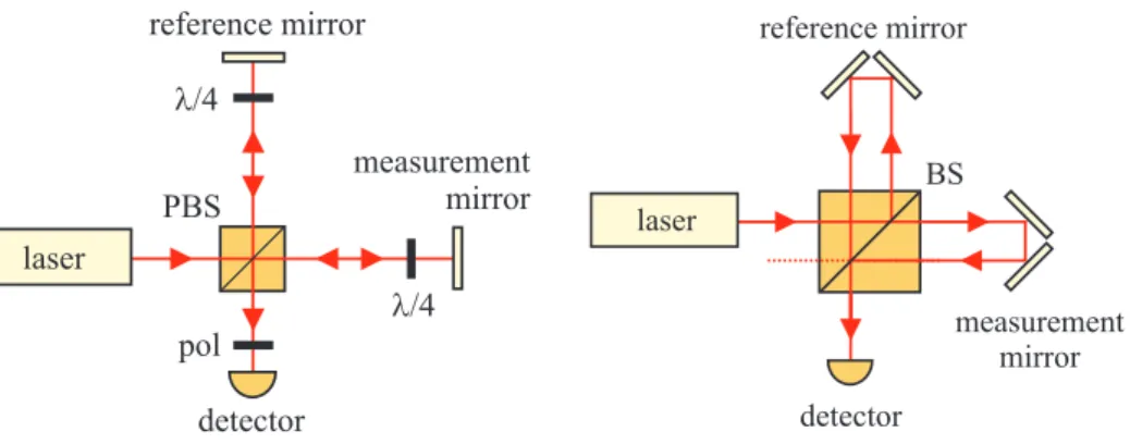
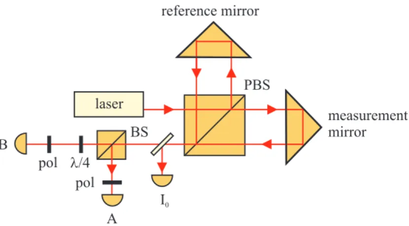
3.3.2. Interferometric Measurement

Single-path interferometers as Michelson and Mach-Zehnder interferometers are state of the art technologies which are highly developed in a variety of different implementations. Such interferometers offer pm-accuracy – demonstrated in lab experiments. A tilt measurement can be implemented by performing a spatially resolved phase measurement, e.g. with quadrant photodiodes (Differential Wave- front Sensing, DWS [51, 52]). A schematic of a Michelson interferometer with a proof mass acting as measurement mirror is shown in Fig. 3.3 (b). A more detailed

(36)

PSD proof laser 1 mass

detector frequency lock

beat

measurement laser 2

frequency lock

Figure 3.4.: Multiple-path interferometry.

analysis concerning single-path interferometry will be given in chapter 4.

Multiple-path interferometry, i. e. the use of optical resonators (cavities) is most promising, providing the highest sensitivity in position sensing. A possible implementation is shown in Fig. 3.4. The resonance frequency f_resof a cavity with length Lis given by

f_res= nc

2L, (3.7)

wherecis the vacuum speed of light and n an integer number. A laser frequency locked to the resonance frequency of a cavity will change its frequency when the length of the resonator is changing. In case of LISA one cavity mirror will be fixed to the satellite structure (i.e. the optical bench or housing), the other mirror is rigidly fixed to the proof mass (e.g. by directly coating the proof mass surface). Locking the laser to this cavity and performing a beat measurement with a second laser which is frequency locked to a stable reference cavity will provide the information on a change in frequency of the first laser and therefore change in lengthL of the corresponding cavity.

Depending on the finesse of the cavity, a sensitivity up to∼1 fm/√

Hz could be achieved. A tilt of the proof mass might be measured by analyzing higher order modes in the cavity. This technology is not yet demonstrated in a lab experiment and is also highly complex (use of several lasers, which are frequency stabilized to several cavities).

(37)

3.3 Optical Readout (ORO) 29 3.3.3. An Optical Readout Developed at the University of Napoli

(Italy)

The method of a lever sensor as optical readout for the LISA inertial sensor is under investigation at the University of Napoli (Italy). Their design is based on the implementation in the current LISA pathfinder gravitational reference sensor design with its vacuum enclosure where it uses available optical accesses. The laser light is reflected twice on the electrodes (acting as mirrors) and once on the proof mass enabling a measurement of the proof mass translation and tilt. The position of the laser beam is monitored by a position sensitive device (PSD), cf. the schematic shown in Fig. 3.5. The measured power spectral density in translation measurement is also shown in Fig. 3.5. They demonstrated a displacement noise below 10⁻⁹m/√

Hz for frequencies>5·10⁻³Hz [53, 54]. This method can presently not provide the sensitivity needed in the LISA science interferometer but can serve as position sensor for DFACS, supporting the capacitive readout.

3.3.4. An Optical Readout Developed at the University of Birmingham (England)

For the LIGO ground-based gravitational wave detector, the University of Birm- ingham set up a homodyne in-quadrature interferometer utilizing polarizing optical components [55]. They developed a compact prototype using a VCSEL (Vertical Cavity Surface Emitting Laser) laser diode. Noise levels below 10⁻¹²m/√

Hz for frequencies >10 Hz were achieved and work is currently under way to optimize their design with respect to the LISA low frequency measurement band, cf. Fig. 3.6.

Due to its design, the interferometer is insensitive to a tilt of the measurement mirror.

3.3.5. An Optical Readout Developed at Stanford University (USA)

An optical readout using a Littrow resonator is developed at the University of Stan- ford. It is based on a LISA gravitational reference sensor design with spherical proof mass as already proposed in [26]. A double-sided grating is implemented in the housing wall enabling an internal interferometric measurement between the GRS and the proof mass (ORO) and an external interferometric measurement between the GRS and the distant spacecraft (cf. Fig. 3.7 and [57, 58, 59]). The optical setup is similar to the tunable external cavity laser diode design in Littrow configuration.

A relative movement of the grating results in a change, both, in amplitude and frequency; this can be converted to a translation measurement. In a laboratory setup, a

(38)

(a)

(b)

Figure 3.5.: Optical readout developed at the University of Napoli. (a) schematic of the setup, front view; (b) PSD of the measured translation [53].

(39)

3.3 Optical Readout (ORO) 31

(a)

(b)

Figure 3.6.: Optical readout developed at the University of Birmingham. (a) schematic of the interferometer; (b) PSD of the measured translation in the LISA frequency band [56].