An Exact Solution Approach for Portfolio Optimization Problems under Stochastic and Integer Constraints
P. Bonami∗, M.A. Lejeune†
Abstract
In this paper, we study extensions of the classical Markowitz’ mean-variance portfolio opti- mization model. First, we consider that the expected asset returns are stochastic by introducing a probabilistic constraint imposing that the expected return of the constructed portfolio must exceed a prescribed return level with a high confidence level. We study the deterministic equivalents of these models. In particular, we define under which types of probability distributions the determin- istic equivalents are second-order cone programs, and give exact or approximate closed-form for- mulations. Second, we account for real-world trading constraints, such as the need to diversify the investments in a number of industrial sectors, the non-profitability of holding small positions and the constraint of buying stocks by lots, modeled with integer variables. To solve the resulting problems, we propose an exact solution approach in which the uncertainty in the estimate of the expected re- turns and the integer trading restrictions are simultaneously considered. The proposed algorithmic approach rests on a non-linear branch-and-bound algorithm which features two new branching rules.
The first one is a static rule, called idiosyncratic risk branching, while the second one is dynamic and called portfolio risk branching. The proposed branching rules are implemented and tested using the open-source framework of the solver Bonmin. The comparison of the computational results obtained with standard MINLP solvers and with the proposed approach shows the effectiveness of this latter which permits to solve to optimality problems with up to 200 assets in a reasonable amount of time.
Keywords: Programming: stochastic, integer: nonlinear, branch-and-bound, Finance: portfolio;
Probability: distributions
1 Introduction
Since Markowitz’ groundbreaking work in portfolio selection [22], portfolio optimization has been re- ceiving sustained attention from both asset liability professionals and academics. All such studies define a portfolio optimization criterion such as mean-variance, mean absolute deviation, value-at-risk, con- ditional value-at-risk, stochastic dominance of first and second order, etc. In this paper, we use the mean-variance approach that studies how risk-averse investors can construct optimal portfolios taking into consideration the trade-off between market volatility and expected returns. Out of a universe ofr risky assets and one non-risky asset characterized by a known returnµ0 that usually reflects the interest rate on the money market, an efficient frontier of optimal portfolios can be constructed. Portfolios on the efficient frontier offers the maximum possible expected return for a given level of risk.
∗IBM TJ Watson Research Center, 1101 Kitchawan Road, Yorktown Heights, NY 10598, USA;pbonami@us.ibm.com
†Tepper School of Business, Carnegie Mellon University, Pittsburgh PA 15213, USA;mlejeune@andrew.cmu.edu
The original Markowitz’ model assumes that the expected returns µ ∈ Rr of the risky assets and the variance-covariance matrix Σ ∈ Rr×r of the returns are known. One of the several formulations of the mean-variance portfolio selection problems involves the construction of a portfolio with minimal risk provided that a prescribed return level R is attained. This model is formulated by the following mathematical program:
minwTΣw
subject toµ0w0+µTw≥R
r
X
j=0
wj = 1 w∈ Rr+1
. (1)
In the problem above, the decision variableswj,j= 1, . . . , rrepresent the proportion of capital invested in the risky asset j while w0 is the fraction of capital invested in the money market. The objective function aims at minimizing the variance of the portfoliowTΣw, and the constraint
w0+
r
X
j=1
wj = 1 (2)
enforces that the sum of the investments is equal to 1. Clearly, the investor can allocate part of the available capitalKto the money marketw0.
In the last decade, there has been much effort devoted to extending Markowitz’ work and making his modern portfolio theory more practical. In this study, we propose models that account for two limitations associated with the mean-variance approach, namely (i) the randomness in the parameters describing the model and (ii) some of the trading restrictions of stock markets.
The classical mean-variance framework relies on the perfect knowledge of the expected returns of the assets and their variance-covariance matrix. However, these returns are unobservable and unknown.
Even obtaining accurate estimates of them is very complicated. Indeed, many possible sources of errors (e.g., impossibility to obtain a sufficient number of data samples, instability of data, differing personal views of decision makers on the future returns [24], etc.) affect their estimation, and lead to what Bawa et al. [3] call estimation risk in portfolio selection. This estimation risk has been shown to be the source of very erroneous decisions, for, as pointed in [7, 10], the composition of the optimal portfolio is very sensitive to the mean and the covariance matrix of the asset returns, and minor perturbations in the moments of the random returns can result in the construction of very different portfolios. Decision- makers would often rather trade-off some return for a more secure portfolio that performs well under a wide set of realizations of the random variables. The need for constructing portfolios that are much less impacted by inaccuracies in the estimation of the mean and the variance of the return is therefore clear.
The focus here is on the uncertainty associated with the estimation of the expected returns. It is indeed a widespread belief among portfolio managers, and its was shown in [9], that the the portfolio estimation risk is mainly due to errors in the estimation of the expected return and not so much to errors in the estimation of the variance-covariance matrix [7]. In this paper, we assume that the expected return
is stochastic and characterized by a probability distribution, and we require that the expected return of the portfolio is larger than a given level with a high confidence level. We show that the associated problem takes the form of a probabilistically constrained problem with random technology matrix [18, 25] that can be reformulated as a nonlinear optimization problem (not necessarily convex). We define under which conditions and for which classes of probability distributions the deterministic equivalent problem is convex and takes the form of a second-order cone problem. We examine in which cases an exact closed-formulation can be derived. If a closed-form formulation cannot be obtained, we provide convex approximations that are obtained by using Chebychev’s inequality [23] and whose tightness depends on the properties of the probability distribution. This convexity analysis of the model gives insights about the applicability and the computational tractability of the proposed model. In related studies, Costa and Paiva [11], T¨ut¨unc¨u and Koenig [31] and Goldfarb and Iyengar [15] have also studied the mean-variance framework in a robust context, assuming that the expected return is stochastic. They characterize the parameters involved in the mean and the variance-covariance matrix with specific types (polytopic, box, ellipsoidal) of uncertainty, and build semi-definite or second-order cone programs. In [12], a risk-averse approach is used for the value-at-risk formulation of the optimization problem, in which only partial information about the probability distribution is known.
The need to account for stock market specifics exacerbates the complexity of the portfolio selection problem. Real-life trading restrictions, such as the minimum amount to invest in an asset, the require- ments to buy assets in large lots, or the purchase of assets in a minimal number of industrial sectors, are not considered in the classical mean-variance models. In the present study, we consider those require- ments that are respectively called buy-in threshold, round lot, and diversification trading constraints. The modeling of such constraints involves the introduction of integer variables and further challenges the computational tractability of the associated problems [10, 29]. In the next paragraph, we proceed to a review of the literature in which the construction of optimal portfolios satisfying such integer constraints is addressed.
Bienstock [5] considers variants of the Markowitz model which features a cardinality constraint and buy-in threshold constraints. He shows that the problem is NP-complete when a cardinality constraint on the number of asset in the portfolio is present. An exact solution framework by branch-and-cut is developed for which computational results on the exact solution of problems with up to 3300 assets are reported. In [17], an exact branch-and-bound solution approach is proposed for problems subject to buy-in threshold, cardinality and round lot constraints. Frangioni and Gentile [14] also consider buy-in threshold constraints, and develop a new family of cutting planes to handle them. Computational results for problems with up to 300 assets are reported. Using mean absolute deviation as optimization criterion, Konno and Yamamoto [19] consider cardinality and fixed transaction cost constraints and solve problems in which up to 54 assets can be included in the portfolio. It is important to remark that all the studies above do not account for the uncertainty in the problem parameters.
To the best of our knowledge, this study is the first one to propose an exact solution approach for portfolio optimization problems in which uncertainty in the estimate of the expected return and real-life
market restriction modeled with integer constraints are simultaneously considered. The combination of integrality and of a probabilistic constraints makes such problems very difficult to solve. Such problems belong to the family of Mixed Integer Non-Linear Programs (MINLP) for which only very few solvers are available. In this paper, we use the computational framework offered by the open-source mixed-integer non-linear solver Bonmin [6]. We propose a non-linear branch-and-bound algorithmic approach, and we develop two new branching rules, called idiosyncratic risk and portfolio risk branching rules. Extended computational experiments on problems containing up to 200 assets clearly show the effectiveness and utility of the two new branching rules. The reader will note that, although the results reported in the paper are obtained for one of the variants of the probabilistic Markowitz’ model (i.e., risk minimization subject to the attainment of a predefined return level1), the proposed solution approach can be easily extended to the other variants.
The paper is organized as follows. In the first part of Section 2, we describe the characteristics of the constraint enforcing that the portfolio return exceeds with a probabilitypa given prescribed return level.
We present the problem formulation and its deterministic equivalent, we study under which condition it is convex, and we propose exact or approximate closed-form formulations of the deterministic equivalent problem. The second part of Section 2 is devoted to the formulation of the integer constraints and models associated with three types of trading restrictions. Section 3 describes the proposed solution approach.
Section 4 reports and comments the computational results. Section 5 provides concluding remarks and suggests extensions to the proposed study.
2 Problem formulation and properties
2.1 Probabilistic portfolio optimization model
The proposed portfolio optimization model takes the form of a probabilistically constrained optimization model with random technology matrix. We refer the reader to the seminal papers of Kataoka [18] and van de Panne and Poppe [25] for a first study of such stochastic programming models in applications pertaining to the transportation and diet problems, and to [8, 16, 26, 33] for more recent studies.
We denote byξthe random vector of return of therrisky assets;ξhas anr-variate distribution with mean
µ= (µ1, µ2, . . . , µr)T , µj =E(ξj), j = 1, . . . , r, and variance-covariance matrix
Σ =E[(ξ−µ)(ξ−µ)T]. The probabilistic constraint
P
µ0w0+
r
X
j=1
ξjwj ≥R
≥p (3)
in which the coefficients ξ multiplying the decision variables w are stochastic and not (necessarily) independent, guarantees that the expected return of the portfolioµ0w0+
r
P
j=1
ξjwjis above the prescribed
minimal level of returnRwith a high probabilityp, typically defined on[0.7,1).
The stochastic version of Markowitz’ mean-variance portfolio optimization problem [22] reads:
minwTΣw subject toP
µ0w0+
r
X
j=1
ξjwj ≥R
≥p
w0+
r
X
j=1
wj = 1 w∈ Rr+1+
. (4)
The decision variables are given by ther+ 1-dimensional vectorwof portfolio positions. We recall that w0 is the proportion of the available capitalK invested in the money market with fixed returnµ0,wj, j = 1, . . . , ris the proportion of the capitalKinvested in the risky assetj,ξj is the stochastic return of assetj,Σis the variance-covariance matrix of the returns, and the objective functionwTΣwrepresents the variance of the portfolio. In our model, we assume that the variables are positive, not allowing short-selling positions. This constraint can be removed without affecting the nature of the problem.
2.2 Deterministic equivalent
We shall first show that the deterministic equivalent of the probabilistic portfolio optimization model is a nonlinear programming optimization problem.
Defining byψ= ξT√w−µTw
wTΣw the normalized (i.e., mean 0 and variance 1) random variable representing the expected portfolio return, it follows that
P(ξTw≥R) =P
ψ≥ R−µTw
√ wTΣw
= 1−F
R−µTw
√ wTΣw
, (5)
where F is the cumulative probability distribution of the (normalized) portfolio return andF−1 is its inverse. Therefore, the probabilistic constraint (3) becomes
1−F
R−µTw
√ wTΣw
≥p
⇔F
R−µTw
√ wTΣw
≤1−p
⇔µTw+F−1(1−p)
√
wTΣw≥R
, (6)
whereF−1(1−p)is the(1−p)-quantile ofF.
The deterministic equivalent of (4) is the following nonlinear optimization problem:
minwTΣw
subject toµTw+F−1(1−p)
√
wTΣw≥R w0+
r
X
j=1
wj = 1 w∈ Rr+1+
. (7)
In the next-subsections, we shall study under which conditions, i.e. for which classes of probability distributions the above problem is a second-order cone optimization problem (and is therefore convex, and solvable in polynomial time). We shall see that it is not possible to derive an exact closed-form formulation of the second-order cone problem for each probability distribution. We shall, therefore, using Chebychev’s inequality, derive closed-form approximations of the second-order cone problem that are valid for some families of probability distributions.
2.2.1 Convexity results
a) Symmetric probability distributions
The probability distribution F of a random variable ξ is symmetric around its mean µ if P(ξ ≥ µ+b) =P(ξ ≤ µ−b),b ∈ R, and is centrally symmetric ifP(ξ ≥b) =P(ξ ≤ −b). We provide a more formal definition below.
Definition 2.1 A probability distribution of an r-variate random vector is centrally symmetric if its density functionf is such thatf(A) =f(−A)for all Borel setsA⊆ Rr.
Theorem 2.2 Ifp∈ [0.5,1)and if the probability distribution ofξTwis symmetric, the deterministic equivalent µTw+F−1(1−p)
√
wTΣw ≥ R of the probabilistic constraintP(ξTw ≥ R) ≥ p is a second-order cone constraint.
Proof. The matrix of variance-covarianceΣis positive semidefinite, and thus the function
√ wTΣw is convex. To show thatµTw+F−1(1−p)√
wTΣw ≥ R is a second-order cone constraint whose feasible set is convex, it is enough to prove that the function µTw+F−1(1−p)
√
wTΣwis concave, which is the case ifF−1(1−p)is smaller than or equal to 0.
Since the probability distribution ofξ is symmetric, the probability distributionF of the normalized random variableψis centrally symmetric. It follows thatF(0) = 0.5(or, equivalently, thatF−1(0.5) = 0). This, combined with the fact that any cumulative distribution function is increasing, implies that F−1(1−p), p∈[0.5,1)is at most equal to 0, which was set out to prove.
Clearly, problem (7) minimizes a convex quadratic function over a second-order cone and some linear constraints, and is therefore a convex, second-order cone problem.
b) Positively skewed probability distributions
The skewness is a measure of the asymmetry of a probability distribution of a real-valued random variable [1], and is computed as
skew(ξ) = E[ξ−µ]3 σ3 , whereµandσare respectively the mean and standard deviation ofξ.
The probability distribution F of a random variable is said to be right-skewed or to have positive skewness (left-skewed or negative skewness, respectively) if the right, upper value (left, lower value,
resp.) tail is longer or fatter than the left, lower value (right, upper value, resp.), or, stated differently, if its medianmis strictly smaller (larger, resp.) than its meanµ.
m m
Figure 1: Skewed probability distributions
The two graphs above illustrate the notion of skewness. Both probability distribution functions have the same expectation and variance. The one on the left is positively skewed, while this on the right is negatively skewed.
Definition 2.3 The probability distribution of anr-variate random vectorξhas positive skewness if P(0≥ψ)≥P(m≥ψ)⇔F−1(α)≤0, α≤0.5
whereE[ψ] =E[ξ−µ] = 0andF(m) =P(m≥ψ) = 0.5.
Theorem 2.4 If p ∈ [0.5,1)and if the probability distribution of ξTw has positive skewness, the deterministic equivalent µTw+F−1(1−p)
√
wTΣw ≥ R of the probabilistic constraint P(ξTw ≥ R)≥pis a second-order cone constraint.
Proof. As mentioned above,µTw+F−1(1−p)
√
wTΣw≥Ris a second-order cone constraint if F−1(1−p)(p≥0.5)is smaller than or equal to 0.
This follows immediately from Definition 2.3:
0> F−1(1−p),1−p≤0.5
for the probability distributionF of the normalized random variableψhas positive skewness.
The exact value of the quantileF−1(1−p)can be derived for some probability distributions. If we assume the returns of the risky assets to be normally distributed, then the normalized portfolio returnψ has a standard normal cumulative distribution function
φ(ψ) = 1
√2π Z ψ
−∞
e−t2/2dt ,
and the numerical value of its quantileφ−1(p)is known. The same applies if the normalized portfolio return is uniformly distributed in an ellipsoidΩ ={ω =Qz:kzk ≤1}withkzkdenoting the Euclidian norm ofz.
2.2.2 Quantile approximation
The exact value of the(1−p)-quantileF−1(1−p)cannot be derived for each probability distributionF which therefore impedes the derivation of the exact deterministic equivalent of the probabilistic constraint (3) in (4). In this section, using variants of Chebychev’s inequality, we derive convex approximations of (3) for different classes of probability distributions. Such approximations are popular in the robust optimization literature [4], and differ in terms of their conservativeness.
Theorem 2.5 The second-order cone constraint
µTw− r p
1−p
√
wTΣw≥R is a valid approximation of the probabilistic constraint
P ξTw≥R
≥p (8)
when the portfolio return follows any probability distribution characterized by its first two momentsµ andσ2.
Proof. Let us consider the random variableY such thatYTw= (2µT−ξT)w:YTwhas the same mean and variance thanξTw.
Applying Chebychev’s inequality, we obtain P YTw−µTw > µTw−R
≤
1 1+(µT w−R)2
wTΣw
= wTΣw+(µwTΣwTw−R)2 ifµTw≥R
1 otherwise
. (9) Clearly,
P YTw−µTw > µTw−R
=P µTw−YTw < R−µTw
=P ξTw−µTw < R−µTw . This, combined with (9), successively implies that
P ξTw−µTw < R−µTw
≤ wTΣw
wTΣw+ (µTw−R)2 1− P ξTw−µTw≥R−µTw
≤ wTΣw
wTΣw+ (µTw−R)2 P ξTw−µTw≥R−µTw
≥1− wTΣw
wTΣw+ (µTw−R)2 (10) Therefore,
1− wtΣw
wtΣw+ (µTw−R)2 ≥p
is sufficient for constraint (8) to hold. The expression above can be successively rewritten as:
(1−p) wTΣw+ (µTw−R)2
≥wTΣw (1−p) (µTw−R)2 ≥p wTΣw
µTw− r p
1−p
√
wTΣw≥R
which was set out to prove.
A tighter approximation can be obtained if the probability distribution is symmetric.
Theorem 2.6 The second-order cone constraint
µTw− s
1 2(1−p)
√
wTΣw≥R is a valid approximation of the probabilistic constraint
P ξTw≥R
≥p when the portfolio return has a symmetric probability distribution.
Proof. Chebychev’s inequality for symmetric probability distributions is formulated as follows:
P ξTw−µTw > µTw−R
≤ (
0.5·min h
1,(µwTw−R)TΣw 2
i
ifµTw≥R
1 otherwise , (11)
where the expressionmin[a, b]returns the minimum value ofaandb Consequently, we have that
1−1 2
wTΣw
(µTw−R)2 ≤P ξTw−µTw≤µTw−R , and, using the same variable substitution approach as above, we obtain
P ξTw−µTw≥R−µTw
≥1−1 2
wTΣw
(µTw−R)2 . (12) Therefore,
1−1 2
wTΣw
(µTw−R)2 ≥p is a sufficient condition forP ξTw≥R
≥pto hold true. Consequently, 2 (µTw−R)2 ≥ wTΣw
1−p µTw−
s 1 2(1−p)
√
wTΣw≥R
which was set out to prove.
2.3 Integrality constraints for stock market restrictions
We now propose extensions of problem (7) in order to take into account real-life stock market restrictions.
These are modeled through the introduction of integer decision variables in (7), and pertain to prevention from holding small positions (Section 2.3.1), to the requirement of purchasing shares by batch of a certain size (Section 2.3.2), and to the investment in a predefined minimal number of industrial sectors (Section 2.3.3).
This leads to the formulation of integer convex probabilistic problems whose deterministic equiva- lents are second-order cone mixed-integer problems whose general formulation is given below:
minwTΣw
subject toµTw+F−1(1−p)
√
wTΣw≥R, gj(w, y)≤0, j= 1, . . . , m w∈ Rr+1+ ,
y ∈ Z+.
(13)
Problem (13) minimizes the volatility of the portfolio over a convex feasible set determined by the second-order cone constraint on the expected return andmdeterministic constraintsgj(w, y)≤0. The decision variablesyare integer-valued.
2.3.1 Buy-in threshold constraints
In this section, we introduce constraints that prevent investors from holding very small active positions.
The rationale for this hinges on the fact that such small positions have very limited impact on the total per- formance of the portfolio [29], but trigger some tracking and monitoring costs. Certain portfolio selection models, such as the Markowitz model, are known for occasionally returning an optimal portfolio contain- ing very small investments in a (large) number of securities. Such a portfolio is in practice very difficult to justify due to the costs of establishing and maintaining it (brokerage fees, bid-ask spreads, etc.), and the usually poor liquidity of small positions. In order to avoid this, constraints preventing from holding an active position representing strictly less than a prescribed proportionwminof the available capital are useful. To model such constraints, we introducerextra binary variablesδj ∈ {0,1}, j = 1, . . . , rtaking value 1 if the investor detains shares of assetj(i.e.,wj >0):
wj ≤δj, j = 1, . . . , r . (14) Small investments are avoided by introducing the following constraints:
wminδj ≤wj , j= 1, . . . r . (15)
With these additional variables and constraints, problem (13) becomes minwTΣw
subject toµTw+F−1(1−p)
√
wTΣw≥R w0+
r
X
j=1
wj = 1 wj ≤δj , j= 1, . . . , r wminδj ≤wj, j = 1, . . . r δ ∈ {0,1}r
w∈ Rr+1+
. (16)
2.3.2 Round lot purchasing constraints
Large institutional investors usually purchase large (i.e., even lot) blocks of individual financial assets.
This is primarily because such blocks are more easily traded than smaller (i.e., odd lot) holdings, but also for liquidity reasons, i.e., to avoid the risk of getting stuck with a small, poorly liquid holding of a financial asset. Another reason to buy stocks by lots of large quantity is that, often, brokers require a premium for odd lot trades because they may have to split an even lot which would leave them with the remaining odd lot part. This is what motivates the construction of portfolio optimization models including round lot constraints that require the purchase of shares by batches or lots ofMstocks.
To each risky assetj, we associate a general integer variableγj, and a round lot constraint
xj =γjM , j= 1, . . . , r (17) imposing that the numberxj of shares of asset j in the portfolio is a multiple ofM. Denoting by pj
the face value of stockj and byK the available capital, it follows thatxj = wpjK
j . We can therefore reformulate (17) as
wj = pjγjM
K , j= 1, . . . , r .
Problem (13) becomes a second-order cone problem with general integer decision variables minwTΣw
subject toµTw+F−1(1−p)
√
wTΣw≥R w0+
r
X
j=1
wj = 1 wj = pjγjM
K , j= 1, . . . , r γ ∈ Z+r
w∈ Rr+1+
. (18)
2.3.3 Diversification constraints
Many institutional investors have limitations on the allowable exposure to risky investments. Very often, such limits are defined by an upper bound on the maximum percentage of the portfolio value that may be invested in certain categories of financial assets, and/or by the requirement to invest in a predefined minimum number of asset categories or industrial sectors. In this section, we consider constraints that force the investor to diversify its portfolio by purchasing assets in at least Lmin different economic sectors. Every assetj is linked with an economy sectork, so that the setsSk, k = 1, . . . , Lof assets affiliated with a sectorkform an exact partition of{1, . . . , r}. We associate a binary variableζk∈ {0,1}
with each economic sectork:ζkis equal to1if and only if the investment in sectork( P
j∈Sk
wj) is above a minimum pre-defined levelsmin:
smin ζk≤ X
j∈Sk
wj ≤smin+ (1−smin) ζk. In addition to the constraint above we must add a cardinality constraint
L
X
k=1
ζk≥Lmin
to satisfy the diversification requirement.
The diversification condition requires to detain ”representative” positions in at leastLminsectors. Note that the constraints above do not consider a very small position in a sectork(i.e.,≤smin) as contributing to the diversification of the portfolio. The probabilistic Markowitz model with diversification constraint reads:
minwTΣw
subject toµTw+F−1(1−p)
√
wTΣw≥R w0+
r
X
j=1
wj = 1 sminζk≤ X
i∈Sk
wk≤smin+ (1−smin)ζk, k= 1, . . . , L
L
X
k=1
ζk ≥Lmin
ζ ∈ {0,1}L w∈ Z+r+1
(19)
3 Solution Method
In this paper, we develop an exact Mixed-Integer Non-Linear Programming (MINLP) solution method for portfolio optimization problems subject to the joint enforcement of probabilistic constraint on the expected portfolio return and integer constraints representative of trading mechanisms. More precisely,
we rely on a non-linear branch-and-bound algorithm that we complement with new branching rules, namely the idiosyncratic risk and portfolio risk branching rules.
The proposed solution approach is implemented within the open-source solver Bonmin [6, 2] (avail- able under the Common Public License) designed to solve to optimality general MINLP of form
minf(x)
subject to gi(x)≤0, ∀i= 1, . . . , m xi ∈ Z, ∀i∈I
x∈Rn,
wheref : Rn → Randgi : Rn → Rm are at least once continuously differentiable convex functions.
Several algorithm can be chosen in Bonmin for solving MINLP and the reader is referred to [6] for a detailed description of the algorithms and their implementation. In our case, preliminary tests indicated that the branch-and-bound was the best method available in Bonmin for solving portfolio optimization problems. In the following, we give a brief reminder of the classical branch-and-bound algorithm used in Bonmin and then describe two new branching rules which are suitable for the considered portfolio optimization problems.
3.1 Non-linear branch-and-bound algorithm
The non-linear branch-and-bound algorithm solves problems of the form (20) by performing an implicit enumeration through a tree search. The algorithm starts by solving the continuous relaxation of (20), where all integrality requirements have been removed, using the interior point solver Ipopt [32]. We de- note by(w∗, y∗)the optimal solution of this continuous relaxation. Ify∗is integer valued, then(w∗, y∗) is the optimal solution and the problem is solved. Otherwise, at least one of the integer variables (yi) has a non integer value. Such a variable is chosen for branching: two sub-problems (or nodes) are created where the upper and lower bounds onyˆiare set tobyˆ∗
icanddyˆ∗
ie, respectively, and the two sub-problems are put in a list of open nodes.
Then, at each subsequent iteration of the algorithm, a sub-problem is chosen from the list of open nodes, and the continuous relaxation of the current node node is solved providing a lower bound. The enumeration at the current node can be stopped, or stated differently, the node is said to be fathomed or pruned, if any of the three following conditions happen:
• the continuous relaxation is infeasible (pruning by infeasibility);
• the optimal solution of the continuous relaxation is not better than the value of the best integer feasible solution found so far (pruning by bounds);
• the optimal solution of the continuous relaxation is integer feasible (pruning by optimality).
If the optimal solution of the continuous relaxation solution(w∗, y∗)cannot be pruned, then at least one of the integer variables (yi) has a non integer value (y∗i 6∈ Z) in the optimal solution. One of the
integer infeasible variablesyˆi cis then chosen for branching, and two new sub-problems are thus added to the list of open nodes. By iterating the process a search tree is created and the algorithm continues until the list of open sub-problems is empty.
One of the key ingredients of the branch-and-bound procedure is the choice of the variable to branch- on. The most classical rule is to choose the variable which has the largest fractional part, but this rule is often not very efficient. In this paper, we present two new rules specifically adapted to the portfolio optimization problems presented in Section 2. These two rules are respectively called idiosyncratic risk and portfolio risk branching and are described in the next sections.
3.2 Static branching rule: Idiosyncratic Risk Branching
The idiosyncratic risk branching rule is a static branching rule in which branching priorities are deter- mined a priori (i.e., before the optimization is started).
For each integer decision variable, the branching priority is given by an integerπi. At each node, the variable chosen for branching is the one, among the integer constrained variables with fractional value in the optimal solution of the current continuous relaxation, which has the highest priority. In case of a tie (i.e., when several candidate variables for branching have the same priority), the variable selected for branching is the one among those with highest priority which is the most fractional in the continuous relaxation.
It is important to recall that, in the optimization problems with buy-in threshold constraints (16) and with round lot constraints (18), there is a mapping between assets and integer decision variables: to each assetjcorresponds a unique integer decision variableδj in (18) andγj in (16). In the context of mean- variance portfolio optimization problems, we propose to give the highest priority to the integer decision variable associated with the asset whose return has the greatest variance. We refer thereafter to this branching procedure as the idiosyncratic risk branching procedure. The intuition behind these priorities is that the asset with the largest variance is the one which has the most significant impact on the overall risk of the portfolio. Therefore, if the variance is the largest, the two sub-problems resulting from the branching are more likely to have an optimal value differing substantially from that of the parent node.
For the problems with diversification constraints, each integer decision variable is associated with a specific industrial sector. To each binary variable, and therefore to each sector, we assign a branching priority which is an increasing function of the sum of the variances of each asset stock related to the considered sector.
3.3 Dynamic branching rule: Portfolio Risk Branching
The portfolio risk branching rule is a dynamic branching rule, in which the branching priorities change at each node and tributary of the structure of the portfolio at the current node. Clearly, the branching vari- able is determined by relying upon a dynamic, integrated risk approach. The dynamics of the branching rule stems from the revision of the branching priorities at each node in the search tree, while its integrated
risk approach derives from the fact that the branching priorities are a function of the specific contribution of each variable (asset) to the overall risk of the portfolio.
The dynamic feature is relevant since, in the course of the optimization process, a new optimal portfolio can potentially be constructed at each node in the branch-and-bound tree. Therefore, an iterative (at each node) evaluation of the contribution of each variable to the variance of the portfolio is desirable.
As it will be detailed in the next subsections, it is possible to establish a direct correspondence between an integer decision variable and an asset. At each node in the branch-and-bound tree, we consider each integer variable whose optimal value in the current continuous relaxation is not integer feasible. For each such variable, we evaluate how the restoration of the integrality condition impacts (increases) the variance of the current portfolio. The variable whose integer feasibility restoration has the largest impact on the variance receives the highest priority, and is the one with respect to which we branch.
To carry out this evaluation, we approximate the problem at hand by a more simple disjunctive program with quadratic objective function and linear equality constraints which takes into account the integrality of only one variable:
minf(w) =wTΣw subject toAw=b,
(wi ≤wi)∨(wi≥wi), i∈1, . . . , r w∈ Rr
(20)
Clearly, the problem above, and therefore the evaluation of the impact of the integer feasibility restora- tion, are obtained by omitting the non-linear term in the portfolio return constraint and relaxing the bounds on the variables.
In the next subsections, we give a precise description of how this approximation is obtained for each variant of the probabilistic Markowitz problem. Prior to this, we explain how the branching rule is ap- plied in the general setting of (20).
Letw∗ be the (continuous) optimal solution of (20), and letLλ(w)be the Lagrangian function:
Lλ(w) =f(w) +λT(Aw−b). (21) We estimate the change in the objective value of (20) through the Lagrangian function. A movement ofδ∈ Rrfromw∗ induces the following change in (21):
Lλ(w∗+δ)− Lλ(w∗) = (w∗+δ)TΣ(w∗+δ)−w∗TΣw∗+λT(Aδ)
=δTΣδ+ (2w∗TΣ +λTA)δ . Sincew∗is optimal, it satisfies the KKT conditions:
2w∗TΣ +λTA= 0 λ(Aw∗−b) = 0
which implies thatLλ(w∗+δ)− Lλ(w∗) =δTΣδ.
Let us consider a variablewi with valuew∗i, such thatw∗i ∈ [wi, wi]. Branching onwi creates two nodes: in each of them we add one of the constraints wi ≤ wi andwi ≥ wi. Using the procedure described above, we estimate the change in the Lagrangian of (20) by computing the two estimatesδi− andδi+defined by
δi−= (wi∗−wi)eTi Σ(w∗i −wi)ei = (wi∗−wi)2σii
δi+= (wi−wi∗)eTi Σ(wi−w∗i)ei = (wi−w∗i)2σii
(22) whereeiis a vector whose components are all equal to0but thei−th one which is equal to1.
By analogy to mixed-integer programming [21], we then combine these two estimates to obtain the score of variablewiby taking a linear combination of the minimum and the maximum of the two [21]:
δi =Lmin(δi−, δ+i ) +Umax(δi−, δi+). (23) We set the values ofLto1andU to2.
We calculateδifor all integer variables with fractional values in the optimal solution of the continu- ous relaxation, and we select as branching variable the one which has the highest score:
ˆi= arg max
{i:w∗i∈(wi,wi)}δi.
The quality of the branching scheme depends on the quality of the relaxation (20) with respect to the original problem. For the problems handled in this paper, it is easy to build such relaxations, and the computational experiments indicate that they are of good quality.
3.3.1 Problem with buy-in threshold constraints
In this section, we discuss the implementation of the dynamic portfolio risk branching rule in problem (16) in which the constraints (14) and (15) define the minimum proportion of available wealthK that must be invested in any active position.
In this case, we use the following formulation:
minwTΣw
subject toµTw+F−1(1−p)
√
wTΣw≥R w0+
r
X
j=1
wj = 1 (wi≤0)∨(wi ≥wmin) w∈ Rr+1+
. (24)
Note that this formulation is strictly equivalent to (16): imposing the conditionwi ≤0is equivalent to settingγito0in (16) and imposingwi≥wminis equivalent to settingγito 1. The continuous relaxation is obtained by removing the disjunctive constraints.
The selection of the branching variable is performed by applying the scheme described in Section 3.3 to the following relaxation
minwTΣw subject toµTw=R
w0+
r
X
j=1
wj = 1 (wi ≤0)∨(wi≥wmin) w∈ Rr+1
of problem (24). The relaxation is obtained by transforming the portfolio return constraint into an equal- ity constraint from which the non-linear component is dropped, and by removing the non-negativity constraints.
3.3.2 Problem with round lot constraints The constraintγi = M pK
iwiestablishes a direct correspondence between the continuous variableswj and the integer onesγj in portfolio optimization problems with round lot constraints (18). Therefore, for a particular value ofw∗, we use the following relaxation
minwTΣw subject toµTw=R
w0+
r
X
j=1
wj = 1
(wi≤ K
M piwi∗
)∨(wi ≤ K
M piw∗i
)
, (25)
to select the branching variable in portfolio optimization problems with round lot constraints (18).
4 Computational results
4.1 Test problems
To build the test bed for our approach, we use the daily return data of more than 600 stocks that have been part of Standard&Poor’s 500 index between 1990 and 2004. The data accounts for the splits that the considered stocks have undergone in the period indicated above. Based on the time series, we calculate the estimates of the geometric mean of the returns and their variance-covariance matrix.
Using those data, we build 36 portfolio optimization instances of various sizes (12 problems with 50 assets,12 with100and12with 200) by randomly selecting the assets included in those problems.
For each problem instance, we formulate three models corresponding to the trading constraints (buy-in threshold, round lot purchase, and diversification) considered in this paper. To model the problems with
diversification constraints, we use the Global Industry Classification Standard (GICS) [30] developed by S&P and Morgan Stanley Capital International to identify the industrial sector to which each company belongs. The GICS structure consists of 10 Sectors, 24 Industry Groups, 67 Industries and 147 Sub- Industries. The present study allocates each company to one of the 67 industries. The data come from the CRSP database and were obtained using the Wharton Research Database Service.
In each problem instance, the prescribed return level R is set equal to 7%, the fixed return of the money market is equal to 2% and the prescribed reliability level p,by which the investor wants the expected portfolio return to exceed the prescribed return level, is set to 85%. The asset returns are assumed to follow a normal distribution. The problem instances are modeled by using the Ampl modeling language.
In our experiments, we compare MINLP BB[20] and the default branch-and-bound algorithm of Bonmin[6] to our specialized branch-and-bound algorithms implemented within the Bonmin framework.
MINLP BB uses a branch-and-bound method and solves the continuous relaxations with a sequential quadratic trust region algorithm called filterSQP[13]. Some of main differences between MINLP BB and Bonmin are:
• MINLP BB uses an active set method for solving the continuous relaxation while Bonmin uses an interior point algorithm,
• MINLP PP uses the depth-first search strategy for choosing the next node to process in the tree search (i.e., it selects the deepest node for processing next) while Bonmin, by default, uses best- bound (i.e., the next node to be processed is chosen as the one whose parent provides the smallest lower bound).
All tests were performed on an IBM IntellistationZ Pro with an Intel Xeon 3.2GHz CPU, 2 gigabytes of RAM and running Linux Fedora Core 3.
4.2 Evaluation of solution approaches 4.2.1 Model with buy-in threshold constraints
In this section, we analyze the computational results obtained for the problem instances containing buy-in threshold constraints. The experiments have been conducted by setting the minimum fraction of wealth (wmin) to be invested in an asset (should the investor decide to include that asset in his portfolio) equal to2%,3%and5%for the instances with50,100and200stocks, respectively.
Table 5 reports the results obtained with the four solution approaches listed below on the 36 problem instances with buy-in threshold constraints:
• Bonmin’s branch-and-bound algorithm with branching performed on the most fractional integer variable (i.e., the default branching rule in Bonmin),
• Bonmin’s branch-and-bound algorithm with the idiosyncratic risk branching rule (Section 3.2),
• Bonmin’s branch-and-bound algorithm with the portfolio risk branching rule (Section 3.3.1),
• MINLP BB’s branch-and-bound algorithm.
The above solution approaches will thereafter be referred to as MF, IR, PR, and MBB, respectively.
For each ”combination” of problem instance and solution approach, Table 5 reports
• the quality of the best obtained solution (columns 2, 5, 8, 11). We use the acronym ”NS” to indicate that no feasible integer was found. We report the value of the mixed-integer optimality gap when the best integer solution found is not optimal, and use the symbol ”*” when the optimal solution is found;
• the computing time (in CPU seconds) needed to find the optimal solution (columns 3, 6, 9, 12).
If this latter cannot be found within the allowed computing time (3 hours), the entry in the table reads ”>10800”;
• the number of explored nodes in the branch-and-bound tree (columns 4, 7, 10, 13);
First, we comment on the accuracy of the solutions found. It is well known that the structure of the variance-covariance matrix of returns often leads to numerical difficulties [5]. While we can not exactly establishing the optimality of the obtained solutions, outside of the tolerances of the solvers, we can compare the values of the optimal solutions obtained with Bonmin and with MINLP BB; we recall that bot solvers are based on very different continuous nonlinear programming methods. We observe that the relative difference between the optimal solutions found by Bonmin and MINLP BB are in the order of 10−4except for problem 050 1 where it is8.56∗10−3(note that the solution found by the three variants of Bonmin are always identical for these instances as well as for all the other instances in the paper). It is also worth pointing out that the solution claimed by Bonmin always has a better objective value than the one claimed by MINLP BB on these problems.
The instances with 50 and 100 do not really allow us to discriminate the four solution approaches in terms of the quality of the solution. Indeed, Figure 2 shows that the optimal solution is found by each solution approach for each 50-stock and 100-stock problem instance.
For the most complex problems containing 200 stocks, the solution approaches IR and PR utilizing the two new proposed branching rules clearly dominate M P andM BB. The former two approaches solve each instance to optimality, while the latter two solve only 25% of those instances to optimality. It is also worth noting that MP does not find any integer feasible solution when it cannot find the optimal one, while MBB always finds an integer feasible solution, and has an average optimality gap of 5.29%.
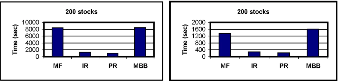
Figures 3 and 4 display the average computing time for each combination of solution approach and size of problem instance.
In Figure 4, the left-sided graph shows the average time computed over 200-stock instances, while the right-sided one shows the average time computed over the only instances that could be solved to optimal- ity by every solution approach. It is clear that the solution approachesIRandP Rrelying respectively
0%
20%
40%
60%
80%
100%
MP IR PR MBB
Dimension of problem Op tim
al so lut ion
50 stocks 100 stocks 200 stocks
Figure 2: Quality of solution for problems with buy-in constraints
50 stocks
500 100150 200250
MF IR PR MBB
Time ( sec)
100 stocks
2000 400600 1000800 1200
MF IR PR MBB
Time ( sec)
Figure 3: Average computing time for 50-stock and 100-stock instances with buy-in constraints
on the idiosyncratic and portfolio risk branching rules are, regardless of the size of the problem, much faster thanM P andM BB. TheP Rsolution approach is slightly faster thanIR, and is on average more than 5 (respectively, 17 and 25) times faster thanM BBon 50-stock (respectively, 100- and 200-stock) instances.
Figure 5 shows the evolution of the average computing time (for all instances on the left-hand side, for instances solved to optimality on the right-hand side). We can see that PR and IR scale very well:
the rhythm at which their average computing time increases is very reasonable, therefore indicating their applicability to problems of larger size. This must be contrasted to the MF and MBB approaches for which the computing time seems to increase exponentially in the number of assets.
4.2.2 Model with round lot constraints
Table 5 reports the computational results for the 36 problem instances with round lot constraints and in which the investor is constrained to buy shares by multiples ofM set equal to 100 in our experiments.
Table 5 provides the same outputs (optimality gap, CPU time, number of nodes) and uses the same notations as those of Table 5. The following four integer solution methods have been tested:
200 stocks
20000 40006000 100008000
MF IR PR MBB
Time ( sec)
200 stocks
4000 1200800 16002000
MF IR PR MBB
Time ( sec)
Figure 4: Average computing times for 200-stock instances with buy-in constraints
0 200 400 600 800 1000 1200 1400 1600
50 100 150 200
Number of stocks Time
MF IR PR MBB
0 1000 2000 3000 4000 5000 6000 7000 8000
50 100 150 200
Number of stocks Time
MF IR PR MBB
Figure 5: Buy-in constraints: computing time as a function of dimensionality
• Bonmin’s branch-and-bound algorithm with branching on the most fractional integer variable,
• Bonmin’s branch-and-bound algorithm with the idiosyncratic risk branching rule (Section 3.2),
• Bonmin’s branch-and-bound algorithm with the portfolio risk branching rule (Section 3.3.2),
• MINLP BB’s branch-and-bound algorithm.
Figure 7 shows that the IP solution approach using the dynamic portfolio risk branching rule is by far the most robust method for problems with round lot constraints. The IP method is the only one solving to optimality all 100-problem instances, and finds the optimal solution for 83% of the 200-problem instances, while none of the three other methods can solve to optimality any of those twelve problem instances. A few additional comments are in order. First, the MF approach does not find any feasible integer solution for any of the problem instances that it cannot solve to optimality (i.e., 43% and 100% of the 100-stock and 200-stock instances, respectively). The IR does not find any integer feasible solution for any of the 200-problem instances. On the other hand, MBB always finds a feasible integer solution, and has an average optimality gap of 0.204% and 1.039% for the 100-stock and 200-stock instances, respectively.
0%
20%
40%
60%
80%
100%
MF IR PR MBB
Dimension of problem Op tim
al so lut ion
50 stocks 100 stocks 200 stocks
Figure 6: Quality of solution for problems with round-lot constraints
Figure ?? shows that PR is not only the most robust but also the fastest regardless of the dimensional- ity of the problem. The average computing times (i.e., irrespective of whether one considers all instances [left-side in Figure ??] , or only those solved to optimality by all approaches [right-side in Figure ??]) of PR are very significantly lower than those of the other methods. It appears that the difference in speed between PR and any of the other three methods increases with the size of the problem; indeed, PR is
• 1.22 (instances solved to optimality) and 1.44 (all instances) times faster than MBB (the second- fastest method) for the 50-stock instances;
• 3.65 (instances solved to optimality) and 10.62 (all instances) and times faster than MBB for the 100-stock instances.
No speed comparison can be drawn for the 200-stock instances since PR is the only method solving some (83%) of them to optimality.
0%
20%
40%
60%
80%
100%
MF IR PR MBB
Dimension of problem Op tim
al so lut ion
50 stocks 100 stocks 200 stocks
Figure 7: Quality of solution for problems with round-lot constraints
Finally, we note that the relative difference between the optimal values found by Bonmin and MINLP BB are always smaller than10−4. In all but 6 cases the value found by Bonmin is better than the one found by MINLP BB. In those 6 cases where MINLP BB finds a better solution the largest relative difference is2∗10−5.
4.2.3 Model with diversification constraints
The results displayed in Table 5 are related to the 36 problem instances with cardinality-type diversifica- tion constraints.
The results have been obtained by settingLmin(the minimum number of sectors in which the investor must allocate his capital) to 10, 15 and 20 for the problem instances comprising 50, 100 and 200 assets, respectively, and by settingsmin (minimal position in any of theKmin sectors) to1%for all problem instances. The results obtained with the following three integer solution methods
• Bonmin’s branch-and-bound algorithm with branching on the most fractional integer variable,
• Bonmin’s branch-and-bound algorithm with the idiosyncratic risk branching rule (Section 3.2),
• MINLP BB’s branch-and-bound algorithm are given in Table 5.
The results in Table 5 indicate that the three methods above solve to optimality all 36 instances in very limited computing time. The average computing times for the slowest and fastest methods (respectively MF and MBB) are equal to 126 sec and 69 sec. Clearly, the problems with diversification constraints appear the easiest to solve.
The relative difference between the optimal values found by Bonmin and MINLP BB is again in the order of10−4and the solution found with Bonmin is always smaller than that obtained with MINLP BB.
4.3 Impact of integer trading constraints
We discuss below the impact on the various types of integer trading constraints. In particular, we analyze
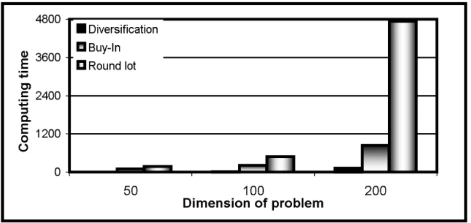
• the difficulty of solving the problem associated with each type of constraints. The difficulty is evaluated with respect to the average computing time per type of models and for each problem size (50, 100, 200 stocks). Figure 8 shows that the computational time is an increasing function in the number of stocks, and highlights the following hierarchy in terms of problem complexity:
1. problem with cardinality constraints, 2. problem with buy-in threshold constraints, 3. problem with round lot constraints.
0 1200 2400 3600 4800
50 100 200
Dimension of problem Co mp
uti ng tim e
Diversification Buy-In Round lot
Figure 8: Average computing time per model type and problem dimension
The largest problems (i.e., 200-stock instances) with diversification constraints require less com- puting time on average than the least complex (i.e., 50-stock instances) problems with round lot constraints. The accrued complexity of those latter is due to the presence of general integer vari- ables which implicitly require the detention of an integer number of shares of any asset included in the optimal portfolio.
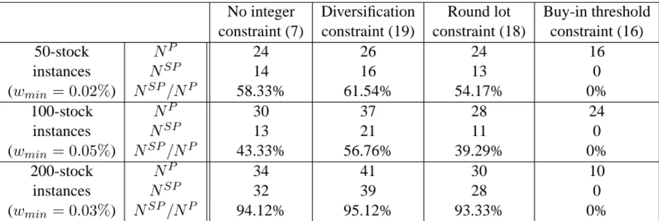
• the impact of the buy-in threshold constraints. Table 1 presents detailed results about the composi- tion of the optimal portfolio for each combination of model type (without integer constraints, with diversification, round lot and buy-in threshold constraints) and problem size. The notationNP and NSP respectively denote the average number of positions in the optimal portfolio and the average number of positions which are greater than the threshold imposed by the buy-in constraints. The thresholdwminis equal to 2%, 3% and 5% for the 50-, 100- and 200-stock instances, respectively.
Table 1 shows that the buy-in constraints drastically change the structure of the optimal portfolio.
The optimal portfolio with buy-in constraints is less diversified than the optimal portfolio obtained with any of the other three approaches. The optimal portfolio with buy-in constraints has positions in 16, 24 and 10 assets for 50-, 100- 100-, and 200-stock instances, respectively. These number must be contrasted to those of the optimal portfolios without any integer constraints (24, 30, 34), with diversification constraints (26, 37, 41), and with round lot constraints (24, 28, 30).
• the impact of the diversification constraints. In addition to constraining the holding of positions in a pre-defined number of industrial sectors, the diversification constraints, as shown by Table 1, have also for effect that the investor detains positions in a larger number of assets (at least, on average, 20.5% of the available assets) and detains a larger number of small positions (at least, on average, 56.76%).
• the impact of the round lot constraints. The requirement to buy shares by large lots has for effect to limit the number of active positions which is smaller than that for the model without integer