Non-convex Feedback Optimization with Input and Output Constraints for Power System Applications

(1)

Research Collection

Master Thesis

Non-convex Feedback Optimization with Input and Output Constraints for Power System Applications

Author(s):

Häberle, Verena Publication Date:

2020-04-17 Permanent Link:

https://doi.org/10.3929/ethz-b-000410529

Rights / License:

In Copyright - Non-Commercial Use Permitted

This page was generated automatically upon download from the ETH Zurich Research Collection. For more information please consult the Terms of use.

(2)

The text font of “Automatic Control Laboratory” is DIN Medium C = 100, M = 83, Y = 35, K = 22

C = 0, M = 0, Y = 0, K = 60

Logo on dark background K = 100 K = 60 pantone 294 C

pantone Cool Grey 9 C

Automatic Control Laboratory

Master Thesis

Non-convex Feedback Optimization with Input and Output Constraints for Power

System Applications

Verena Häberle April 17, 2020

Advisors

Prof. Dr. F. Dörfler, Dr. S. Bolognani, A. Hauswirth, L. Ortmann

(3)

(4)

Abstract

In this thesis, we present a novel control scheme for feedback optimization. That is, we propose a discrete-time controller that can steer the steady state of a physical plant to the solution of a constrained optimization problem without numerically solving the problem. Our controller can be interpreted as a discretization of a continuous-time projected gradient flow and only requires reduced model information in the form of the steady-state input-output sensitivity of the plant.

Compared to other schemes used for feedback optimization, such as saddle-point flows or inexact penalty methods, our scheme combines several desirable properties: It asymptotically enforces constraints on the plant outputs, and temporary constraint violations along the trajectory can be easily quantified. Further, as we prove in our main result, global convergence to a minimum is guaranteed even for non-convex problems, and equilibria are feasible regardless of model accuracy. Additionally, our scheme is straightforward to tune, since the step-size is the only tuning parameter. Finally, we numerically verify robustness (in terms of stability) of the closed-loop behavior in the presence of model uncertainty.

For the envisioned application in power systems, we use our novel feedback approach to steady- state optimization for time-varying AC power flow optimization. In numerical experiments, we show that our scheme scales nicely for larger power system setups and exhibits robustness with respect to time-varying generation limits, unobserved demand variations, and a possible model mismatch.

(5)

(6)

Preface

I would like to express my gratitude to Dr. Saverio Bolognani, Adrian Hauswirth and Lukas Ortmann for supervising and guiding me through this master thesis. I highly appreciate their enormous readiness to help, along with their fast and elaborate responses to all my questions.

Furthermore, I want to thank for their professional advice as well as for sharing their immense knowledge of the field during our regular weekly meetings. Thanks to their inspiring and mo- tivating way of supervision, I really enjoyed contributing to the ongoing research on feedback optimization for power systems.

My special gratitude goes to Adrian Hauswirth, who invested a lot of time for additional discus- sions and brainstorming sessions on relevant mathematical technicalities.

Likewise, I want to thank Professor Dr. Florian Dörfler who made it possible to work on this project. Im a very grateful for his outstanding quality of advice during personal meetings and especially for his insightful comments on the draft of my first L-CSS/CDC submission¹.

Last but not least, I would like to acknowledge the support of the scientific and administrative staff at the Automatic Control Laboratory (IfA), on whom I could always rely throughout the entire project.

1IEEE Control Systems Letters (L-CSS) and 59^th Conference on Decision and Control (CDC), 2020, Jeju Island, Korea

(7)

(8)

List of Figures

3.1 Feedback optimization setup where the controller is provided with the closed-loop measurement of the system output at steady state. . . 11 4.1 Left: infeasible equilibrium u⁺ of the “relaxed” direct forward Euler integra-

tion (4.1) (u^? denotes the equilibrium of the continuous-time projected gradient flow (3.4)); Right: bounded residual error of the “relaxed” direct forward Euler integration (4.1) at the equilibrium u⁺. . . 15 4.2 Trajectory of the projected forward Euler integration (4.3) with Euclidean projec-

tion of the integration pointu−α∇Φ˜ onto the feasible setU˜. . . 16 4.3 One-dimensional example for the LOPG iteration with projection onto the lin-

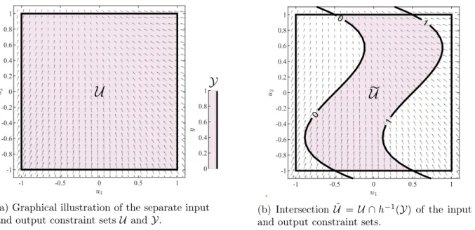
earized setU˜_u at each iterate. Left: side view; Right: aerial view. . . 18 4.4 Components of the setU˜. The vector field represents the negative gradient−∇Φ(u). 24˜ 4.5 Comparison of the LOPG iteration scheme with the direct forward Euler integration. 25 4.6 Variation of the iteration step sizeα of the LOPG iteration scheme. . . 26 4.7 Comparison of the LOPG iteration scheme with a penalty approach for different

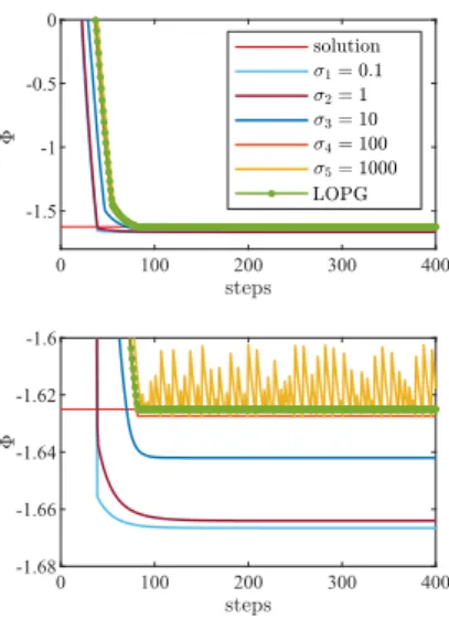
penalty parametersσ. . . 27 4.8 Comparison of the LOPG iteration scheme with an augmented saddle-point method

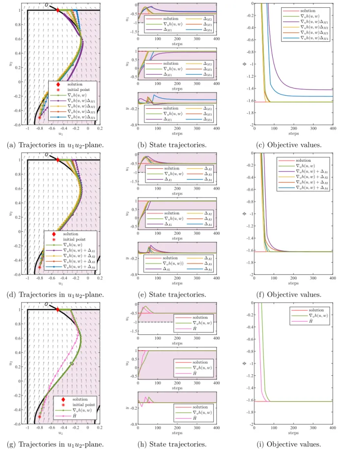
for different dual step sizes γ and fixed augmentation parameterρ= 1. . . 27 4.9 LOPG iteration scheme for different estimations H(∆). . . .ˆ 30 5.1 3 bus power system with controllable set-points of each bus. . . 37 5.2 Simulation results of controlled 3 bus power system with novel LOPG iteration

scheme. The dashed lines represent the constraints and the colors are the same as in Table 5.2. The iteration step size is fixed toα= 0.0002. . . 38 5.3 Simulation results of controlled 3 bus power system for penalty approach and

augmented saddle-point method. The dashed lines represent the constraints and the colors are the same as in Table 5.2. The iteration step size is fixed toα= 0.0002. 40 5.4 Modified IEEE 30 bus power flow test case. . . 41 5.5 Simulation results of controlled 30 bus power system for the exact Jacobian matrix

∇_u,yF(u, y, w)and a constant approximation thereof. The dashed lines represent the constraints and the colors are the same as in Table 5.3. . . 43 A.1 Comparison of the new scheme for different metrics. . . 54 B.1 Instabilities for a too large iteration step sizeα= 0.02. The dashed lines represent

the constraints and the colors are the same as in Table B.1. . . 55

(11)

(12)

List of Tables

4.1 Tuning parameters of different control approaches and impact on the performance characteristic. . . 28 5.1 Partition of state variables by bus type, adpated from [13]. . . 32 5.2 Cost coefficients a and b in[$/MW²h] and [$/MWh], respectively. Active power

generation limits in [MW], reactive power generation limits in [MVAr], and bus voltage limits in [p.u.]. The system base power is fixed to100MVA. . . 37 5.3 Cost coefficients a and b in[$/MW²h] and [$/MWh], respectively. Active power

generation limits in [MW] and reactive power generation limits in [MVAr], and bus voltage limits in [p.u.]. The system base power is fixed to 100MVA. . . 41 B.1 Cost coefficients a and b in [$/MW²h] and [$/MWh], respectively. Active and

reactive power generation limits in [MW] and [MVAr], and bus voltage limits in [p.u.]. The system base power is fixed to100MVA. . . 56

(13)

(14)

Chapter 1 Introduction

In recent years, the design of feedback controllers that steer the steady state of a physical plant to the solution of a constrained optimization problem has garnered significant interest both for its theoretical depth [6, 19, 23, 28] and potential applications. The historic roots of feedback optimization trace back to process control [7, 10] and the study of communication networks [20, 25]. More recent efforts have centered around the application to power systems, where feedback optimization is used for frequency control [24, 38], voltage control [4, 30, 34] or power flow optimization [8, 13, 33]. In particular, real-time algorithms for time-varying AC optimal power flow (AC OPF) have recently attracted lots of interest, as fast control capabilities are required to handle the increased volatility and randomness in power systems, for which traditional optimal power flow methods are inappropriate.

We adopt the perspective that feedback optimization emerges as the interconnection of an optimization algorithm such as gradient descent (formulated as an open system) and a physical plant with well-defined steady-state behavior. In particular, we assume that the plant is stable and exhibits fast-decaying dynamics. Motivated by previous work on timescale separation in these setups [16, 27], we can abstract the system by its steady-state behavior, which can be represented by an algebraic input-to-output map y = h(u, w), determined by the controllable input u and some unknown exogenous inputw (e.g. plant parameters, power loads ...).

The critical aspect of feedback optimization is that, instead of relying on a full optimization model, the controller is provided with the closed-loop measurements of the system output y.

This entails that the system model h does not need to be known explicitly, nor does it need to be evaluated numerically. Instead, only information about the steady-state sensitivity∇h is required, which is generally available for practical applications. This renders feedback optimization schemes inherently more robust against disturbances and model uncertainties than conventional

“feedforward” numerical optimization.

A particular challenge in feedback optimization is the incorporation of (unilateral) constraints on the input and output of the plant. Input constraints can usually be enforced directly by means of projection or by exploiting physical saturation and using anti-windup control [12, 17]. On the other hand, output constraints cannot be enforced directly, especially when the plant is subject to some unknown exogenous input. In particular, constraints on the transient plant dynamics are very hard to enforce. In feedback optimization, we therefore only deal with constraints on the steady-state output of the plant. Previous works on feedback optimization either considered inexact penalty methods [13, 33] or saddle-point flows [6, 8, 24]. The former treat the output constraints as soft constraints using penalty functions, while the latter ensure the constraints to be satisfied asymptotically, i.e., at the steady state of the feedback dynamics. However, saddle- point flows exhibit oscillatory behavior in their trajectories, are difficult to tune, and do not come with strong guarantees for non-convex problems.

(15)

In this thesis, we present a new way of enforcing output constraints in feedback optimization by establishing a novel discretization of projected gradient flows. As we prove in or main result, for a small enough iteration step size, global convergence is guaranteed even for non-convex problems, and equilibria are feasible regardless of model accuracy. Inspired by numerical algorithms like sequential quadratic programming (SQP) [2, 29], our discretiztion scheme works by project- ing gradient iterates onto a linearization of the feasible set around the current state and then applying them as set-points to the system. This concept has also been explored in [35], where global convergence is proven via a line-search argument based on a variable step-size. In our setup, however, we cannot rely on line-search techniques, and instead, have to establish global convergence for fixed step-sizes. Furthermore, we need to ensure that our optimization scheme admits an implementation as a feedback controller.

Compared to inexact penalty approaches, our scheme guarantees that output constraints are satisfied asymptotically. This is similar to saddle-point schemes. However, in contrast to saddle- point flows, our scheme exhibits a benign convergence behavior without oscillations (which we illustrate with numerical examples), temporary constraint violations along the trajectory are quantifiable, convergence is guaranteed for non-convex problems, and tuning is restricted to a single parameter.

Our novel control strategy to steady-state optimization is scalable for larger power systems, where the feedback optimization task is formalized as an AC OPF, which is not required to be solved explicitly. Namely, the feedback-optimizer is designed such that the non-linear AC power flow equations are enforced naturally by the laws of physics, requiring no computational effort. We show in two numerical experiments how time-varying AC OPF problems can be solved by using our new feedback approach that steers the power system to an optimal state under stationary conditions. More precisely, we analyze the closed-loop behavior under time-varying generation limits and discuss robustness towards unmeasured demand variations and model uncertainty. In particular, even at fast-changing conditions, our control scheme proves to be able to accurately track the time-varying optimal operating point of the system, while enforcing operational constraints along the system trajectories. Similar experimental studies based on slower timescales have been performed in [13, 33], however, the corresponding algorithms treat the endogenous operational constraints as soft constraints by using penalty functions, which generally results in residual constraint violations.

The rest of this thesis is structured as follows.

• In Chapter 2, we fix the notation and summarize relevant results from variational geometry, perturbed optimization problems, dynamical systems, and projected gradient flows.

• Chapter 3 presents the concept of feedback optimization in continuous time.

• In Chapter 4, we present our novel discrete-time controller and prove our main convergence result. In simple numerical simulations, we show typical performance characteristics of the new scheme, and in particular discuss its robust nature with respect to model uncertainty.

• The application of our scheme to power systems is analyzed in Chapter 5, where we consider time-varying AC power flow optimization with fluctuating load and generation limits, and illustrate the resulting closed-loop behavior in two numerical power system examples.

• Finally, we summarize our main conclusions in Chapter 6, and briefly address future work.

• In Appendix A, we provide an additional convergence proof for an alternative discrete-time feedback optimization approach, which relies on the full knowledge of the model.

(16)

• Furthermore, in Appendix B, we illustrate that a too large iteration step size causes our controller to fail.

(17)

(18)

Chapter 2 Preliminaries

2.1 Notation and Technical Results

ForRⁿ,h·,·idenotes the Euclidean inner product and||·||its induced 2-norm. The closed (open) unit ball of appropriate dimension is denoted by B (intB). The non-negative orthant of Rⁿ is written asRⁿ_≥0 and the set of symmetric positive definite matrices of sizen×nis denoted bySⁿ₊. Any G∈Sⁿ+induces a 2-norm defined as ||v||_G:=

√

v^TGv for allv∈Rⁿ. Given a set C ⊂Rⁿ, a mapG:C →Sⁿ+ is called ametric onC.

Derivatives

For a continuously differentiable function f :Rⁿ → R^m, the matrix ∇f(x) ∈ R^m×n of partial derivatives denotes the Jacobian of f at x. The Jacobian at x with respect to a variable x⁰ is given by∇_x⁰f(x). Based on this, we write ∇_x⁰_{, x}⁰⁰f(x) to specify the Jacobian atx with respect to two variablesx⁰ andx⁰⁰. The mapf isglobally L-Lipschitz continuous if for allx, y∈Rⁿ and some L >0, it holds that||f(x)−f(y)|| ≤L||x−y||.

In the following, we present two principal theorems relating to differential functions, which we require for our purpose in this thesis. Namely, we recall the the so-called Descent Lemma [3, Prop A.24].

Lemma 2.1 (Descent Lemma). Given a continuously differentiable function f :Rⁿ → R with L-Lipschitz derivative ∇f, for allx, z ∈Rⁿ it holds that

f(z)≤f(x) +∇f(x)(z−x) +^L₂||z−x||². (2.1) Further, under a mild conditions on the partial derivatives of a function, the set of zeros of a system of equations is locally the graph of a function. This is captured in the so-called Implicit Function Theorem [3, Prop A.25].

Theorem 2.2 (Implicit Function Theorem). Let f :Rⁿ×R^m → R^m be a function of x ∈ Rⁿ and y∈R^m such that

• f(¯x,y) = 0,¯

• f is continuous, and has a continuous and nonsingular gradient matrix ∇_yf(x, y) in an open set containing (¯x,y).¯

Then there exist open sets S_¯_x ⊂ Rⁿ and S_¯_y ⊂ R^m containing x¯ and y, respectively, and a¯ continuous function h : S_¯_x → S_y_¯ such that y¯ = h(¯x) and f(x, h(x)) = 0 for all x ∈ S_x_¯. The function h is unique in the sense that if x ∈ S_¯_x, y ∈ S_y_¯, and f(x, y) = 0, then y = h(x).

Furthermore, if for some p >0, f isp times continuously differentiable, the same is true for h, and we have

∇h(x) =−(∇_yf(x, h(x)))⁻¹∇_xf(x, h(x)), for all x∈ S_¯_x. (2.2)

(19)

Euclidean Projection

For all x ∈ Rⁿ, the Euclidean projection of the vector x onto the set C ⊂ Rⁿ is given by the set-valued map

PC:Rⁿ⇒C x7→arg min

z∈C

kx−zk². (2.3)

IfP_C(x) contains one and only one vector z, i.e., it is single-valued, we simply write¯ P_C(x) = ¯z.

2.2 Variational Geometry

For the continuously differentiable functions k : Rⁿ → R^m and g : Rⁿ → R^p, we consider constraint set of the form

X :={x∈Rⁿ|k(x) = 0, g(x)≤0}. (2.4) Let I^X_x :={i|g_i(x) = 0} denote theindex set of active inequality constraints of X at x and let

¯I^X_x :={i|gi(x)<0}be the index set ofinactive inequality constraints atx.

Definition 2.3 (LICQ). Given X ⊂Rⁿ as in (2.4), the linear independence constraint qualifi- cation (LICQ) is said to hold atx∈ X, if

rank

∇k(x)

∇g_IX x(x)

=m+|I^X_x|. (2.5)

Tangent and Normal Cones

The following definitions comply with the notions from [31, Ch.6]. Given a set X ⊂ Rⁿ, its tangent coneT_xX at a pointx∈ X is, intuitively speaking, defined as the set of directions from which one can approach x from within X. More precisely, w ∈ TxX if there exist sequences x_k →x withx_k ∈ X for allkandδ_k →0⁺such that ^x^k_δ^−x

k →w. For sets of the form (2.4) and if LICQ holds,T_xX takes an explicit form as captured by the following definition [31, Thm 6.31]:

Definition 2.4. Consider a setX of the form (2.4) satisfying LICQ for allx∈ X. The tangent cone of X at x is given by

TxX :={w∈Rⁿ| ∇k(x)w= 0,∇g_IX

x(x)w≤0}.

For sets of the form (2.4) and if LICQ holds, we can define the normal cone as follows.

Definition 2.5. Consider a set X of the form (2.4) satisfying LICQ for all x ∈ X. Given a metric G, the normal cone at x∈ X with respect toG can be defined as

N_xX :={η∈Rⁿ| ∀w∈T_xX :hw, ηi_G(x)≤0}.

Note that, under the given assumptions onX,T_xX andN_xX are closed and convex for allx∈ X. Non-linear Optimization

For a continuously differentiable function Ψ : Rⁿ → R and X ⊂ Rⁿ as in (2.4), consider a non-linear, non-convex constrained optimization problem of the form

minimize

x Ψ(x) subject to x∈ X. (2.6)

TheLagrangian of (2.6) is defined as

L(x, λ, µ) := Ψ(x) +λ^Tk(x) +µ^Tg(x) (2.7) for allx∈Rⁿand all Lagrange multipliers λ∈R^m andµ∈R^p_≥0. Recall the standard first-order optimality conditions (KKT-conditions) for (2.6) [26, Ch. 11.8]:

(20)

Theorem 2.6 (KKT). If x^? ∈Rⁿ solves (2.6) and LICQ holds at x^?, then there exist unique λ^?∈R^m and µ^?∈R^p_≥0 such that

∇_xL(x^?, λ^?, µ^?) = 0, and µ^?_i = 0 for all i∈¯I^X_x?. (2.8) In particular, the LICQ assumption guarantees the uniqueness (and boundedness) of the dual multipliersλ^? and µ^? [36].

Prox-Regular Sets

In the following, we introduce the definition of prox-regular sets. For convenience, we restrict ourselves to constraint-defined sets in the Euclidean space, which is sufficient for our purposes.

Nevertheless, prox-regularity of constraint-defined sets in the Euclidean space can be expanded to more general sets in non-Euclidean settings [14, Ch.7.1].

Definition 2.7. Consider a set of the form (2.4) satisfying LICQ andx∈ X. Forγ >0, the set X is γ-prox-regular at x, if all normal vectors at x are γ-proximal, i.e., for η∈N_xX, we have

hη, y−xi ≤γ||η|| ||y−x||² (2.9) for all y∈ X. The set X is γ-prox-regular if it isγ-prox-regular at every x∈ X.

In particular, every constraint-defined set of the form (2.4), wherek:Rⁿ→R^m andg:Rⁿ→R^p have globally Lipschitz derivatives, and LICQ applies, is γ-prox-regular for some γ >0 [14, Ex 7.7].

A key property of prox-regular sets is the existence of a unique projection on the set for every point in a neighborhood of the set. This is made rigorous in the following Proposition [1, Prop 2.3].

Proposition 2.8. The following assertions hold true.

(i) If the set X ⊂ Rⁿ is γ-prox-regular, then for any x ∈ X + _2γ¹ intB the set P_X(x) is a singleton.

(ii) If the set X ⊂ Rⁿ is γ-prox-regular, then for every x ∈ X, P_X(x+v) = x holds for all v∈NxX ∩ _2γ¹ intB. Further, for ally∈ X + _2γ¹ intB, we have y− P_X(y)∈NP_X(y)X. (iii) If the setX ⊂Rⁿ is γ-prox-regular, then the projection x7→ PC(x) is locally Lipschitz on

X +_2γ¹ intB.

2.3 Sensitivity Analysis of Perturbed Optimization Problems

In this section, we consider constrainedparametric non-linear optimization problems of the form minimize

x Ψ(x, ε)

subject to x∈ X(ε) :={x∈Rⁿ|k(x, ε) = 0, g(x, ε)≤0},

(2.10) whereΨ :Rⁿ× T →R,k:Rⁿ× T →R^mandg:Rⁿ× T →R^p are parametrized inε∈ T ⊂R^r. Correspondingly, the (parametrized) Lagrangian of (2.10) is defined as

L(x, λ, µ, ε) := Ψ(x, ε) +λ^Tk(x, ε) +µ^Tg(x, ε) (2.11) for allx∈Rⁿ,λ∈R^m,µ∈R^p_≥0, and ε∈ T.

We are interested in solutions of (2.10) as a function of ε. For this, we consider the following results from [18, Thm 2.3.2, Thm 2.3.3].

(21)

Theorem 2.9. Consider (2.10) and a given ε¯ ∈ T. Let LICQ and KKT hold at x¯^? with Lagrange multipliers¯λ^? ∈R^m andµ¯^? ∈R^p_≥0. Let the so-called second order sufficiency condition be satisfied, i.e.,

z^T∇²_xL(¯x^?,λ¯^?,µ¯^?,ε)z >¯ 0 hold for all z6= 0 for which∇_xk_j(¯x^?,ε)z¯ = 0,for all j= 1, ..., m, and∇_xgi(¯x^?,ε)z¯ = 0,for all i∈ {i|µ¯^?_i >0}.

(2.12) Furthermore, assume that Ψ, k and g are twice continuously differentiable in x, and that Ψ, k, g, ∇_xΨ, ∇_xk, ∇_xg,∇²_xxΨ, ∇²_xxk, and ∇²_xxg are continuous in ε. Then,

a) x¯^? is a strict local minimizer of (2.10), and the associated Lagrange multipliers ¯λ^? andµ¯^? are unique;

b) for ε in a neighborhood of ε, there exists a unique vector function¯ (x^?(ε), λ^?(ε), µ^?(ε)), which is continuousand satisfies the second order sufficiency condition in (2.12)for a local minimum of the problem in (2.10)with εsuch that(x^?(¯ε), λ^?(¯ε), µ^?(¯ε)) = (¯x^?,¯λ^?,µ¯^?) and, hence, x^?(ε) is a locally unique minimizer of (2.10) at a given ε with associated unique Lagrange multipliers λ^?(ε) andµ^?(ε); and

c) LICQ holds atx^?(ε) for εin a neighborhood of ε.¯

If Ψ, k andg are even twice continuously differentiable in both x and εin a neighborhood of x¯^? and ε, then, additionally,¯

d) the vector function (x^?(ε), λ^?(ε), µ^?(ε)) is locally Lipschitz continuous near ε.¯

As a corollary of the previous theorem, we can prove that for convex optimization problems with strongly convex objective function, the solution map is globally well-defined:

Corollary 2.10. Consider (2.10). For all ε∈ T, let

• Ψ, k and g be twice continuously differentiable in x and let Ψ, k, g, ∇_xΨ, ∇_xk, ∇_xg,

∇²_xxΨ, ∇²_xxk, and∇²_xxg be continuous in ε,

• Ψbe strongly convex in x,

• X(ε) be non-empty and convex in x, and

• LICQ be satisfied for all x∈ X(ε).

Then, there exist continuous functions x^? :T →Rⁿ, λ^? :T →R^m and µ^? :T →R^p≥0 such that x^?(ε) is the unique global optimizer of (2.10)for allε∈ T andλ^?(ε) andµ^?(ε)are the associated unique Lagrange multipliers.

If moreover, Ψ, k and g are twice continuously differentiable in both x and εfor all ε∈ T, then the functions x^? :T →Rⁿ, λ^?:T →R^m andµ^? :T →R^p≥0 are locally Lipschitz continuous.

Proof. By assumption, problem (2.10) is feasible for allε∈ T and LICQ holds for all x∈ X(ε) and all ε∈ T. Further, by strong convexity of (2.10) for all ε∈ T, for any given ε¯∈ T, (2.10) has a unique optimizer. Therefore, the solution map ε→ x^?(ε) exists for all ε ∈ T, satisfying KKT and the second order sufficiency conditions in (2.12) (trivially). Namely, the Hessian of the Lagrangian is strictly positive for allx∈ X(ε) and ε∈ T.

By Theorem 2.9, at an optimizer x^?(¯ε) of (2.10) withλ^?(¯ε) µ^?(¯ε) and a given ε,¯ x^?,λ^? and µ^? are continuous for allεin a neighborhood ofε. This applies to all¯ ε¯∈ T, such that around every

¯

ε∈ T, there must exist such a neighborhood. We can conclude thatx^? :T →Rⁿ,λ^? :T →R^m and µ^? :T →R^p≥0 are continuous for allε∈ T.

The latter reasoning holds also true if differentiability with respect toεis imposed such that we can conclude thatx^? :T →Rⁿ,λ^? :T →R^m andµ^?:T →R^p_≥0 are locally Lipschitz continuous for allε∈ T.

(22)

2.4 Dynamical Systems

Continuous-time Dynamical Systems

Given a map R : Rⁿ → Rⁿ and an additional condition x(0) = x0 ∈ Rⁿ, the following initial value problem for the ordinary differential equation system

˙

x=R(x), x(0) =x0 (2.13)

is referred to as a continuous-time dynamical system. An absolutely continuous function x : [0,∞) →Rⁿ withx(0) =x₀ that satisfies x˙ =R(x) almost everywhere, i.e., for all t∈[0,∞) is a complete(Carathéodory) solution of (2.13).

For the given map R :Rⁿ → Rⁿ, a set S ⊂ Rⁿ is invariant, if R(S) ∈ S, i.e., if every solution starting at somex₀∈ S remains in S.

Suppose that (2.13) has an equilibrium point x^?, i.e., R(x^?) = 0. We characterize the stability of the equilibrium point x^? in the sense of Lyapunov, which is captured by the following definition [21, Def 4.1].

Definition 2.11. The equilibrium point x^? of (2.13) is

(i) stableif, for each >0, there is a δ >0 such that ||x(0)−x^?||< δ =⇒ ||x(t)−x^?||< , for all t≥0;

(ii) unstableif not stable;

(iii) asymptotically stable if it is stable and δ can be chosen such that ||x(0)−x^?|| < δ =⇒

t→∞limx(t) =x^?.

Discrete-time Dynamical Systems

Given a map T : Rⁿ → Rⁿ and an additional condition x(0) = x0 ∈ Rⁿ, the following initial value problem for the first-order difference equation system

x⁺=T(x), x(0) =x₀ (2.14)

is referred to as a discrete-time dynamical system. A sequence x={x(k)}_k ∈Nis the solution to (2.14) if x(k) =T^k(x0) for anyk∈N.

In anology to the continuous-time case, for the given map T : Rⁿ → Rⁿ, a set S ⊂ Rⁿ is invariant, ifT(S)∈ S.

SupposeT(x^?) =x^?, that is,x^? is an equilibrium point for the system in (2.14). Stability of the equilibrium point is defined as follows [11, Def 1].

Definition 2.12. : For each initial value x⁰ close enough to x^?, the equilibrium point x^? is (i) stable, if for each > 0, there isδ, such that ||x(0)−x^?|| < δ =⇒ ||x(k)−x^?|| < , for

all k >0;

(ii) unstableif not stable;

(iii) asymptotically stable, if it is stable and δ can be chosen such that ||x(0)−x^?|| < δ =⇒

k→∞lim||x(k)|| →x^?.

For the convergence analysis of discrete-time systems, we require the discrete-time LaSalle In- variance Principle [22, Thm 6.3].

Theorem 2.13 (Invariance Principle). Consider a discrete-time dynamical system x⁺ =T(x) where T :S → S is well-defined and continuous, and S ⊂Rⁿ is closed. Further, let V :S →R be a continuous function such that V(T(x))≤V(x) for all x∈ S. Let x={x₀, x₁, x₂, . . .} ⊂ S be a bounded solution. Then, for some r ∈ V(S), x converges to the non-empty set that is the largest invariant subset of V⁻¹(r)∩ S ∩ {x|V(T(x))−V(x) = 0}.

(23)

2.5 Projected Gradient Flows

Given a setX ⊂Rⁿ of the form (2.4) satisfying LICQ for allx∈ X, a metricG:X →Sⁿ₊, and a vectorz∈Rⁿ, we define the projection operator

Π^G_X[z](x) := arg min

w∈TxX

||w−z||²_G(x), (2.15)

that is, Π^G_X projects z onto the tangent cone of X at x with respect to G. If f : X → Rⁿ is a vector field, we write Π^G_X[f](x) = Π^G_X[f(x)](x) for brevity. Since T_xX is closed, convex and non-empty for all x ∈ X, (2.15) is a convex problem with strongly convex objective, admitting a unique solution for any x∈ X (in particular,w= 0is feasible for allx). Considering a differentiable potential function Ψ :Rⁿ→ R, a projected gradient flow is defined by the constrained, discontinuous ODE

˙

x:= Π^G_X[−grad_GΨ](x), x∈ X, (2.16) where we have applied Π^G_X[·] to the gradient of Ψ in G, which is defined as grad_GΨ(x) :=

G(x)⁻¹∇Ψ(x)^T. Such systems serve to find local minimizers to optimization problems as in (2.6).

Any complete (Carathéodory) solution of (2.16) has to be viable by definition, i.e., x(t) ∈ X for all t≥ 0. The existence of solutions of (2.16), their convergence to critical points, and the asymptotic stability of strict local minimizers of (2.6) is guaranteed by results in [14] which, for our purposes, can be summarized as follows [14, Prop 5.4, Thm 5.5]:

Proposition 2.14. Consider a compact set X ⊂ Rⁿ of the form (2.4) satisfying LICQ for all x∈ X, a continuous metric G:X →Sⁿ₊, and a continuously differentiable functionΨ :Rⁿ→R. Then,

1. for every x(0)∈ X, (2.16)admits a complete solution,

2. every complete solution of (2.16)converges to the set of first-order optimal points of (2.6), i.e., points satisfying (2.8), and

3. if x^? ∈ X is strongly asymptotically stable¹ for (2.16), then x^? is a strict local minimum of (2.6).

Remark 2.15. Note that if in addition to the conditions in Proposition 2.14, the set X is β- prox-regular for some β >0, and both the metricGand the derivative ofΦare globally Lipschitz continuous on X, by the results in [14], the (complete) solution of (2.16)is unique.

1In case of non-unique solutions,strongasympt. stability implies thateverysolution is asympt. stable.

(24)

Chapter 3 Feedback Optimization

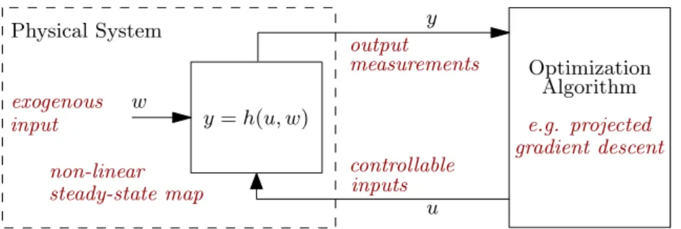
We consider the problem of steering an algebraic physical plant to a steady state that solves a pre-specified (but possibly unknown) constrained optimization problem. The plant has a controllable inputu∈R^p and an uncontrollable exogenous inputw∈R^r (e.g. plant parameters, disturbances,...), which we assume to be constant¹. It is described by a non-linear steady-state input-to-output maph:R^p×R^r→Rⁿ(see Figure 3.1). The assumption that the plant is always at steady state is well-motivated by singular perturbation arguments which can be applied in the context of feedback optimization [16, 27].

Physical System

Optimization

u y

exogenous

controllable inputs non-linear

steady-state map

y=h(u, w) input

Algorithm measurements

output

w

e.g. projected gradient descent

Figure 3.1: Feedback optimization setup where the controller is provided with the closed-loop measurement of the system output at steady state.

3.1 Problem Formulation

For simplicity we consider separate constraints on the inputu∈R^p and the outputy∈Rⁿgiven by polyhedra

U :={u∈R^p|Au≤b} and Y :={y∈Rⁿ|Cy≤d}, (3.1) whereA∈R^q×p, b∈R^q, C ∈R^l×n, and d∈R^l.

Remark 3.1. A generalization of the setY to joint constraints on the input and output is possible at the cost of slightly more involved notation. Nevertheless, for the envisioned applications in power systems, separable constraint sets are sufficiently expressive.

1Note that our control design to steady-state optimization is based on a constantw. However, in our simulations in Chapter 5, we show that our approach also exhibits robustness with respect to a time-varyingw.

(25)

GivenΦ :R^p×Rⁿ→R, we hence consider the problem minimize

u,y Φ(u, y) subject to y=h(u, w)

u∈ U, y ∈ Y.

(3.2)

Solving (3.2) numerically heavily relies on an accurate knowledge of the modelh, including the knowledge of the uncontrollable exogenous inputs w, which are not always available. However, in feedback optimization, an explicit computation ofhis not required, asy=h(u, w)is obtained as the measured system output. Namely, it is enough to know the input-output sensitivity∇_uh (or an approximation thereof), which is usually available in practical applications. Notice also that if the plant’s steady state is linear in u, then ∇_uh(u, w) is constant and therefore known even ifw is unknown.

3.2 Projected Feedback Gradient Flow in Continuous Time

In the following, we consider projected gradient flows as the candidate projected dynamical system to solve (3.2) in closed-loop with the physical plant. Therefore, we first define the desired closed-loop behavior in the input coordinates. By substituting y withh(u, w) in problem (3.2), we arrive at the equivalent problem

minimize

u

Φ(u)˜ subject to u∈U,˜ (3.3)

whereΦ(u) := Φ(u, h(u, w))˜ andU˜:=U ∩h⁻¹(Y). Using (3.3), our desired closed-loop behavior takes the form of the projected gradient flow

˙

u= Π^G_U_˜h

−grad_GΦ˜i

(u), u∈U,˜ (3.4)

where G :U → S^p₊ is a metric and the operator Π^G_U_˜ as defined in (2.15) projects the negative gradient of Φ˜ onto the tangent cone of U˜ at u. Under the following basic assumption, Proposi- tion 2.14 applies and (3.4) is well-posed and converges to first-order optimal points of (3.3).

Assumption 3.2. For the problem (3.3) and the projected gradient flow (3.4) for a given (constant) w,

• the set U is compact,

• the set U˜ is non-empty and satisfies LICQ for all u∈U˜,

• Φ˜ is continuously differentiable and∇Φ˜ is L-Lipschitz on U,

• h is continuously differentiable in u andCi∇_uh is`i-Lipschitz onU for all i= 1, ..., l, and

• G is continuous in u.

The assumption that U is compact is motivated by the fact that physical plants are generally characterized by some physical (actuation) constraints which usually take the form of (non-strict) inequality constraints. Further, it can be shown that the LICQ assumption holds generically [32].

Remark 3.3. To evaluate Π^G_U_˜[−grad_GΦ](u)˜ in (3.4), we require an explicit description of the tangent cone T_uU˜. This is possible under the LICQ condition in Assumption 3.2, which, for U˜:=U ∩h⁻¹(Y), implies

rank

"

A_I^U

u

C_I^Y

h(u,w)

∇_uh(u, w)

#

=|I^U_u|+|I^Y_h(u,w)|. (3.5)

(26)

Consequently, the evaluation of Π^G_U_˜[−grad_GΦ](u)˜ reduces to solving the quadratic program Π^G_U_˜h

−grad_GΦ˜i

(u) = arg min

v∈R^p

grad_GΦ(u) +˜ v

2 G(u)

(3.6a) subject to A_I^U

uv≤0 (3.6b)

C_I^Y

h(u,w)

∇_uh(u, w)v≤0. (3.6c) We reformulategrad_GΦ˜ by applying the chain rule to∇_u(Φ(u, h(u, w))), such that the projected gradient flow (3.4) can be cast as a feedback control system

˙

u= Π^G_U_˜

−G⁻¹(u)H(u)^T∇Φ(u, y)^T

(u) y=h(u, w), (3.7)

wherey is themeasured system output andH(u)^T :=

Ip ∇_uh(u, w)^T .

Since controllers need to be implemented digitally, we now turn to find a proper discretization of the control law in (3.7). However, specific care is needed to deal with the discontinuous nature of Π^G_U_˜, which will be discussed in the following chapter.

(27)

(28)

Chapter 4 Discrete-time Projected Gradient Flow

4.1 Discrete-time Iteration and Practical Implementation

To make (3.7) implementable in practice, we next consider discretizations of the projected gradient flow (3.4) that can be realized as a feedback controller. We aim for a discrete-time controller that does not rely on the explicit knowledge of the full model and instead, preferably uses measurement information. Namely, we propose a discretization of (3.4) which requires limited model information and comes with global convergence guarantees.

4.1.1 Naive Approaches Direct Forward Euler Integration

A natural, albeit naive, idea for discretizing the projected gradient flow in (3.4) consists in a direct numerical evaluation of Π^G_U_˜ as part of the controller, given by the direct forward Euler integration

u⁺=u+αΠ^G_U_˜h

−grad_GΦ˜i

(u), (4.1)

where α is a (fixed) step size. This approach, however, is not well-posed, because it is in general not possible to guarantee that u⁺ ∈ U˜, which is required to be able to compute Π^G_U_˜[−grad_GΦ](u˜ ⁺) at the next iteration. A straightforward extension to still assure well- posedness could be to “relax” the definition of the projection operatorΠ^G_U_˜ in (3.6), by considering

U ˜ U ˜

u⁺

u

−grad_GΦ(u)˜

u^?

u u⁺ u^?

−grad_GΦ(u)˜

αΠ^G_U_˜[−grad_GΦ](u)˜

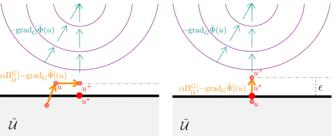
Figure 4.1: Left: infeasible equilibriumu⁺of the “relaxed” direct forward Euler integration (4.1) (u^?denotes the equilibrium of the continuous-time projected gradient flow (3.4)); Right: bounded residual error of the “relaxed” direct forward Euler integration (4.1) at the equilibriumu⁺.

(29)

not only the index sets of active constraintsI^U_u andI^Y_h(u,w)to compute the tangent cone, but the index sets ofactive and violated constraints, given by

ˇI^U_u ={u|Au≥b},

ˇI^Y_h(u,w)={u|Ch(u, w)≥d}. (4.2)

However, apart from the fact that this only works for polyhedral constraints, the “relaxed”

discrete-time system (4.1) might exhibit an equilibrium point outside of the feasible set U˜ (see Figure 4.1, left). The residual erroris bounded by < αM, where M >0 is the upper bound

||grad_GΦ(u)||˜ < M on U, which exists, since grad_GΦ(u)˜ is continuous on the compact set U. Hence, the residual error can be made arbitrarily small by choosing a very small step size α(see Figure 4.1, right). A numerical example based on the direct forward Euler integration in (4.1) is provided in [15].

Nevertheless, the direct (numerical) evaluation ofΠ^G_U_˜ as part of the controller is in general quite expensive, because the tangent cone of U˜ needs to be computed at each iteration. Moreover, model uncertainties inh(u, w) and therefore inU˜=U ∩h⁻¹(Y) might lead to significant performance degradation and substantial stability issues of the control system. Therefore, the direct forward Euler integration (4.1) does not serve as a proper discrete-time implementation of (3.4) in practice.

Projected Forward Euler Integration

An alternative, simple and well-established approach to approximate the projected gradient flow system in (3.4) (but only in the caseG≡I) is theprojected forward Euler integration

u⁺=P_U_˜

u−α∇Φ(u)˜ ^T

, u∈U˜, (4.3)

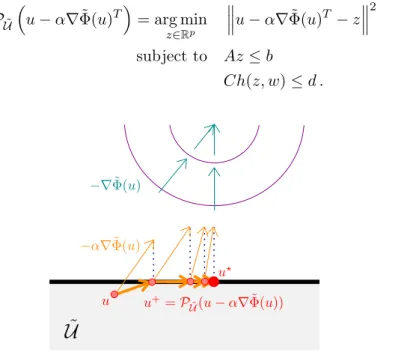
whereαis a (fixed) step size parameter and the map P_U_˜ is defined in (2.3). The system in (4.3) denotes the Euclidean projection of the pointu−α∇Φ˜ onto U˜, which is evaluated as

P_U_˜

u−α∇Φ(u)˜ ^T

= arg min

z∈R^p

u−α∇Φ(u)˜ ^T −z

2

(4.4a)

subject to Az≤b (4.4b)

Ch(z, w)≤d . (4.4c)

U ˜

u u⁺=PU˜(u−α∇Φ(u))˜ u^?

−α∇Φ(u)˜

−∇Φ(u)˜

Figure 4.2: Trajectory of the projected forward Euler integration (4.3) with Euclidean projection of the integration point u−α∇Φ˜ onto the feasible setU˜.

(30)

The main benefit of the system (4.3) is that all iterates are feasible (see Figure 4.2). Moreover, it is shown in Appendix A.1 that for a small enough step size, relying on some key features of prox- regular sets¹, the trajectory of (4.3) globally converges to the set of first-order optimal points of (3.3), and, if an equilibrium is asymptotically stable, it is a strict local minimizer of (3.3).

However, the implementation of this approach is not practical for feedback optimization, as it requires the explicit knowledge of the non-convex setU˜(and thus of the modelh, see (4.4c)), for which robust estimations are generally hard to determine in practical applications.

4.1.2 Proposed Discretization Scheme: LOPG

In the following, we introduce a superior numerical integration scheme for projected gradient flows which, at the same time, admits an implementation as a controller for feedback optimization.

As a starting point, we introduce a custom projection operator Σ^G_U_˜ :R^p×R≥0 → R^p, which is defined as

Σ^G_U_˜[f] (u, α) := arg min

v∈R^p

kf(u)−vk²_G(u) (4.5a)

subject to A(u+αv)≤b (4.5b)

C(h(u, w) +α∇_uh(u, w)v)≤d , (4.5c) where α > 0 is a (fixed) step size parameter and f : U → R^p a continuous vector field. The operator Σ^G_U_˜ can be interpreted as the projection of the point u +αf(u) onto a first-order approximation of the setU˜around the current iterateu. For the feasible set of (4.5), we consider thelinearizedsetU˜_u:=U_u∩ Y_u, where

U_u :={v|A(u+αv)≤b},

Y_u :={v|C(h(u, w) +α∇_uh(u, w)v)≤d}.

For (4.5) to be well-defined, we make the following assumption:

Assumption 4.1. For allu∈ U and a given (constant) w, the setU˜_u is non-empty and satisfies LICQ for allv ∈U˜_u.

Lemma 4.2. Assumption 4.1 implies the LICQ and non-emptiness conditions for the set U˜ in Assumption 3.2.

Proof. Under Assumption 4.1 for anyu∈U˜, it holds that rank

"

A_I^Uu v

C_I^Yu

v ∇_uh(u, w)

#

=|IÛ_vû|+|I^Y_vû|.

At v = 0, IÛ_vû = {j|A_ju = b_j} and I^Y_vû = {i|C_ih(u, w) = d_i} are the index sets of active constraints of U˜_u. Since u ∈ U, we have˜ IÛ_vû ≡ IÛ_u and I^Y_vû ≡ I^Y_h(u,w), and the LICQ condition in Assumption 3.2, as given in (3.5), is satisfied. Further, non-emptiness of U˜ is an immediate consequence of non-emptiness of U˜_u foru∈U˜ at v= 0.

Remark 4.3. Assumption 4.1 is common in the study of SQP methods [2, 29, 35]. Providing sufficient conditions for Assumption 4.1 to hold are subject to future work.

1It can be shown that the non-convex setU˜is prox-regular, which serves as a sufficient condition for uniqueness of the projection on the feasible domainU˜for every point in a neighborhood ofU˜(Propostion 2.8).

(31)

U˜

u

−grad_GΦ(u)˜

u^?

u u⁺

αΣ^G_U_˜[−grad_GΦ](u, α)˜

−grad_GΦ(u)˜

u^? U˜_u

U˜_u⁺

−αΠ^G_˜

U[grad_GΦ](u)˜ u⁺

U˜ U˜_u+

U˜_u d

Ch(u, w)

u

Figure 4.3: One-dimensional example for the LOPG iteration with projection onto the linearized setU˜_u at each iterate. Left: side view; Right: aerial view.

We claim that, for a small α > 0, the so-called Linearized Output Projected Gradient (LOPG) iteration

u⁺=u+αΣ^G_U_˜h

−grad_GΦ˜i

(u, α), (4.6)

approximates the projected gradient flow in (3.4) on U˜. Based on the definition in (4.5), the projected gradient descent step Σ^G_U_˜[−grad_GΦ(u)](u, α)˜ is evaluated as

Σ^G_U_˜h

−grad_GΦ˜i

(u, α) = arg min

v∈R^p

grad_GΦ(u) +˜ v

2 G(u)

(4.7a)

subject to A(u+αv)≤b (4.7b)

C(h(u, w) +α∇_uh(u, w)v)≤d , (4.7c) i.e., Σ^G_U_˜[−grad_GΦ(u)](u, α)˜ projects the point u−αgrad_GΦ(u)˜ onto the linearization of the set U˜ around u (see Figure 4.3). Thus, the LOPG iteration in (4.6) can also be seen as an approximation of the projected forward Euler integration in (4.3). Note that for the LOPG iteration, the set U is invariant by definition. But, due the first order approximation in (4.7c), the trajectory is not necessarily feasible at all iterates (see Figure 4.3). However, it is proven in Section 4.2 that the LOPG iteration converges to feasible first-order optimal points of (3.3) for a small enough step sizeα.

4.1.3 Characteristics of the Projection Operator

Next, we present some fundamental characteristics of the new operator Σ^G_U_˜ with respect to its continuous-time “benchmark” operatorΠ^G_U_˜, which it approximates for a smallα. For a continuous vector field f : ˜U → R^p, we consider a general class of projected dynamical systems and its corresponding discrete-time approximation, given as

˙

u= Π^G_U_˜[f](u) and (4.8)

u⁺=u+αΣ^G_U_˜[f] (u, α), (4.9) respectively². As later shown in Section 4.2, the following characteristics are crucial for the convergence behavior of the discrete-time projected gradient flow in (4.6) when implemented as a feedback controller.

2In our ongoing research, we move towards showing that, as the step sizeαgoes to zero, the discrete-time control law in (4.9) recovers the projected dynamical system in (4.8). More precisely, we consider uniform convergence of the trajectories to the solution of the projected dynamical system in (4.8).

(32)

Besides being well-defined also outside of U˜, the operator Σ^G_U_˜ is continuous inu, coincides with Π^G_U_˜ for all u ∈ U˜ as α → 0⁺, and preserves the same equilibria. This is made rigorous in Proposition 4.4 and 4.5 below. The proofs of these propositions rely on a reformulation of the quadratic problem in (4.5), where the constraints are separated based on whether they are active or inactive constraints of u∈U˜ in (3.3), i.e.,

arg min

v∈R^p

kf(u)−vk²_G(u) (4.10a)

subject to A_I^U

uv≤0 (4.10b)

C_I^Y

h(u,w)

∇_uh(u, w)v≤0 (4.10c)

A¯I^U_uv≤ _α¹(b−A¯I^U_uu) (4.10d) C_¯_I^Y

h(u,w)

∇_uh(u, w)v≤ _α¹(d−C_¯_I^Y

h(u,w)h(u, w)). (4.10e)

Proposition 4.4. Under Assumptions 3.2 and 4.1, the operator Σ^G_U_˜ is continuous in u for all u∈ U. Furthermore, for all u∈U˜,

α→0lim⁺Σ^G_U_˜[f] (u, α) = Π^G_U_˜[f] (u). (4.11) Proof. Continuity ofΣ^G_U_˜ inu can be shown by applying Corollary 2.10 to the problem in (4.5), which is parametrized inu∈ U. We have that for allu∈ U:

• the functions defining (4.5) and their first and second derivatives with respect to v are continuous inu,

• the objective in (4.5) is strongly convex in v,

• the setU˜_u is non-empty and convex in v,

• LICQ is satisfied for allv∈U˜_u.

By Corollary 2.10, v^?(u) is a unique global optimizer of (4.5), which is continuous in u for all u∈ U.

The equivalence in (4.11) can be proven by considering the reformulated problem in (4.10). For α → 0⁺ and u ∈ U˜, the constraints (4.10d) and (4.10e) can be omitted, since their right hand sides tend to +∞. Hence, the constraint set can be reduced to (4.10b) and (4.10c), denoting the tangent cone TuU˜ as given in (3.6b) and (3.6c). Consequently, the reduced problem (4.10a) - (4.10c) is equivalent to the evaluation ofΠ^G_U_˜[f](u).

Proposition 4.5. Under Assumptions 3.2 and 4.1 and givenα >0, ifu^? ∈U˜ is an equilibrium of the discrete-time system (4.9), then u^? is an equilibrium of the projected gradient flow (4.8).

Further, ifu^? is an equilibrium of (4.8), then, for a given α >0, u^? is an equilibrium of (4.9).

Proof. The first statement can be proven by contraposition. Consider an arbitrary feasible point ˆ

u ∈ U, which is not an equilibrium of (4.8), i.e.,˜ vˆ:= Π^G_U_˜[f](ˆu) 6= 0. We can show that uˆ ∈U˜ cannot be an equilibrium of (4.9), i.e. v⁰ := Σ^G_U_˜[f](ˆu, α) 6= 0. For the sake of contradiction, assume Σ^G_˜

U[f](û, α) = 0 at uˆ ∈ U. Note that for the partial problem (4.10a) - (4.10c), being˜ equivalent to the evaluation of Π^G_U_˜[f](û), ˆv 6= 0 is a unique solution. As Σ^G_U_˜[f](û, α) = 0 is assumed, this implies some of the constraints in (4.10d) and (4.10e) are active, i.e. their right- hand sides are equal to zero. However, according to the evaluation ofΠ^G_˜

U[f](ˆu), they are strictly positive at uˆ∈U˜ and we have that the assumption that Σ^G_U_˜[f](ˆu, α) = 0, is false. Therefore, if for a given α >0,u^?∈U˜ is an equilibrium of (4.9), then it is an equilibrium of (4.8).