(wileyonlinelibrary.com)DOI:10.1002/asl.758
Quantifying the extremity of windstorms for regions featuring infrequent events
Michael A. Walz,1,2* Tim Kruschke,2,3Henning W. Rust,2Uwe Ulbrich2and Gregor C. Leckebusch1
1School of Geography, Earth and Environmental Science, University of Birmingham, UK
2Institut fuer Meteorologie, Freie Universität Berlin, Germany
3Department of Ocean Circulation and Climate Dynamics, Research Unit Marine Meteorology, GEOMAR Helmholtz Centre for Ocean Research Kiel, Germany
*Correspondence to:
M. A. Walz, School of Geography, Earth and Environmental Science, University of Birmingham, Birmingham B15 2TT, UK.
E-mail: maw526@bham.ac.uk
Received: 9 December 2016 Revised: 24 May 2017 Accepted: 25 May 2017
Abstract
This paper introduces the Distribution-Independent Storm Severity Index (DI-SSI). The DI-SSI represents an approach to quantify the severity of exceptional surface wind speeds of large scale windstorms that is complementary to the SSI introduced by Leckebuschet al.
While the SSI approaches the extremeness of a storm from a meteorological and potential loss (impact) perspective, the DI-SSI defines the severity in a more climatological perspective.
The idea is to assign equal index values to wind speeds of the same singularity (e.g. the 99th percentile) under consideration of the shape of the tail of the local wind speed climatology.
Especially in regions at the edge of the classical storm track, the DI-SSI shows more equitable severity estimates, e.g. for the extra-tropical cyclone Klaus. In order to compare the indices, their relation with the North Atlantic Oscillation is studied, which is one of the main large scale drivers for the intensity of European windstorms.
Keywords: windstorms; quantification of extremity; North Atlantic Oscillation; extra-trop- ical cyclones; generalized Pareto distribution
1. Introduction and motivation
1.1. Background
Winter windstorms are among the biggest natural haz- ards occurring in the mid-latitudes causing human casu- alties as well as economic losses up to billions of Euros each year. According to SwissRe, the winter storm Kyrill, which strongly affected Central Europe on 18, 19 January 2007 caused an economic insured loss of about $6.1 billion and casualties of 54 people (SwissRe, 2016). An approach to objectively quantify the meteorological hazard is represented by the Storm Severity Index (SSI) introduced by Leckebusch et al.
(2008). The SSI is widely used (e.g. Osinski et al., 2016) for assessing the severity of windstorms within the actuarial sector by linking extreme surface winds (i.e. exceedances of the 98th percentile of local 6-hourly wind speeds) to potential loss on buildings. Further- more, the 98th percentile is used as a criterion for identi- fying extreme windstorms in a wind tracking algorithm by Leckebuschet al.(2008) and further developed by Kruschke (2015). Equation (1) shows the mathemati- cal definition of the SSI. The indextrepresents the time step,krepresents the grid cell andAkrepresents the area of the associated cell divided by a reference cell at the equator:
SSIT,K=
∑T t=1
∑K k=1
[(
max (
0,vk,t−v98,k v98,k
))3
·Ak ]
(1)
Thev98,krefers to the local 98th percentile of thekth grid cell which is the minimum wind speed at which damage on housing or nature is to be expected. This relationship was established based on real damage experience (Klawa and Ulbrich, 2003) which proved the assumption of Palutikof and Skellern (1991) who assumed storm damages to occur at about 2% of all days.
For the further development of the index, the focus will be on the Meteorological ContributionΓto the SSI defined by Equation (2) which shifts and scales wind speeds by the 98th percentile:
Γ = vk,t−v98,k
v98,k (2)
1.2. Motivation for a supplementary severity index (DI-SSI)
Technically, the SSI is based on excesses over a fixed quantile (percentile) for a given wind speed distribution;
however, the SSI does not take into account the shape of the distribution of these excesses, i.e. the tail behaviour.
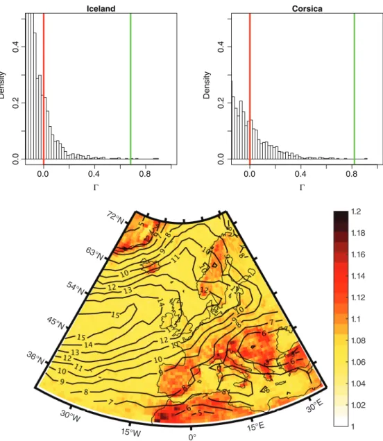
This property becomes particularly obvious in areas with little storm occurrence. The top panel of Figure 1 illustrates this effect: The two panels depict histograms ofΓ(scaled and shifted wind speeds, cf. Equation (2)) of a grid cell south of Iceland (called Iceland hereafter) and on the Isle of Corsica. The coloured lines mark the 98th (red) and the 99th (green) percentile of the shifted and scaled distribution. As known from various
Iceland
Γ
Density
0.0 0.4 0.8
0.00.20.4 Density 0.00.20.4
Corsica
Γ
0.0 0.4 0.8
1.2 1.18 1.16 1.14 1.12 1.1 1.08 1.06 1.04 1.02 1 72°N
63°N
54°N
45°N
36°N
30°W
15°W 15°E
30°E
0°
Figure 1.Top: Histograms of the Meteorological contribution (Γ) as defined in Equation (2) for Iceland (left) and Corsica (right).
The distribution of the events looks visibly different. The red line marks the 98th percentile, thus the cut off threshold. The green line marks the 99th percentile, thus it illuminates the larger difference between the two percentiles for Corsica in comparison with Iceland. Bottom: Quotient between the 99th and the 98th percentile of local wind speeds for Europe in colour. Large values indicate a large difference between the percentiles. The contours depict the average trackdensity per winter (ONDJFM; average number of tracks within a 500 km radius around a given grid point).The quotient is clearly larger in areas with a reduced windstorm frequency.
other studies (e.g. Leckebusch et al., 2008 or Klawa and Ulbrich, 2003) the area south of Iceland is located within the corridor of extra-tropical cyclones (ETCs), whereas Corsica is less affected by ETCs (cf. bottom panel of Figure 1).
By definition of the SSI, the red line is equal to 0.
The histogram for Iceland resembles a light-tailed dis- tribution, whereas the histogram for Corsica shows fea- tures of a heavy-tailed distribution. Accordingly, the gap between the 99th and 98th percentile is substan- tially different (0.68 for Iceland and 0.82 for Cor- sica). Note that due to the cubic relationship of the SSI (Equation (1)), Γ is taken to the third power; for Corsica this is around six times larger thanΓ3for Ice- land (cf. Table 1). From a probabilistic perspective, however, both wind speeds are equally likely. As the
SSI consists of spatially and temporally accumulated Γ3, this implies that a potential storm over Corsica with wind speeds exceeding the 98th percentile will result in a much larger integral SSI value than a storm over Iceland with the same exceptional wind speeds (c.f.
examples for storms Klaus and Martin in Table 2). The gap inΓ3is a direct result of the local wind speed clima- tology and this in turn is a consequence of the scarcity of very extreme winds at the edge of the main storm track.
Thus, within the storm track there are larger ‘back- ground’ winds with a higher number of extreme events, whereas the edges of the storm track feature lower
‘background’ winds and comparatively few extreme events. The exceedance compared with the background wind in relative terms is larger for the edge of the storm track.
80°N
60°N
40°N
80°N
60°N
40°N
80°N
60°N
40°N
80°N
60°N
40°N 80°N
60°N
40°N 80°N
60°N
40°N
30°W 0° 30°E 30°W 0° 30°E
30°W 0° 30°E
30°W 0° 30°E
30°W 0° 30°E 30°W 0° 30°E
Correlation SSI/windstorm frequency Correlation SSI/NAO
Correlation DI-SSI/windstorm frequency Correlation DI-SSI/NAO
Diff correlation DI-SSI–SSI frequency Diff correlation DI-SSI–SSI NAO
0.5 0.3 0.1 –0.2 –0.4 0.7 0.6 0.5 0.4 0.2 –0.2 –0.4 –0.5 –0.6 –0.7
Figure 2.Left panel: Correlation between the storm frequency and storm intensity (SSI on the top; DI-SSI in the middle) for each grid cell. Correlation coefficients significant at the 5% level are stippled. There is a significant link between more storms and more intense storms for much of the North Atlantic and Scandinavia. Right panel: Correlation coefficients between the yearly NAO time series and the yearly windstorm intensity on grid cell level (SSI on the top; DI-SSI in the middle). Again correlation coefficients significant at the 5% level are tagged. Bottom row: Differences between the respective correlations. Positive values represent areas where the correlation for the DI-SSI is larger compared to the SSI. This is the case for most of the North Atlantic Domain.
Table 1.Meteorological and DI-SSI contributions of the two example grid cells. Note that the contribution of the grid cell in Corsica is more than five times larger, although the wind is of the same singularity in both cases.
𝚪3in a single grid cell for a surface wind
equal to the 99th percentile
DI-SSI contribution in a single grid cell for a surface wind equal to
the 99th percentile
Iceland 2.05×10⁻⁴ 0.71
Corsica 1.24×10⁻³ 0.67
Theoretical value – 0.69
The effect of the gaps in the two histograms shown in Figure 1 (top panel) can be shown on grid cell level as well: Figure 1 (bottom panel) depicts the quotient of
the local 99th and 98th percentile (as the division by the 98th percentile is part of the calculation of the SSI) and the average storm frequency per grid cell per extended winter season (i.e. how often on average a windstorm track is detected within a 500 km radius of a particu- lar grid cell). Klawa and Ulbrich (2003) calculated the same quotients for station data of wind speeds in var- ious locations in Germany. Their conclusion was that the quotient was sufficiently homogeneous for the entire country. This assumption can be supported and con- firmed by Figure 1 (bottom). Values above 1.1, how- ever, indicate grid cells which are potentially affected by large SSI values, thus in particular Southern Europe.
These areas coincide with regions of little storminess over the winter period (less than 8–10 windstorm events per year).
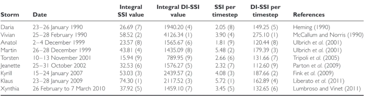
Table 2.Integral SSI and DI-SSI values for some prominent European windstorms. The rank of severity for the respective index is denoted in parenthesis. Note that storms which occurred outside of the main storm tracks feature relatively large SSI values (e.g.
Klaus, Martin, Xynthia, Torsten) compared to the ones within the main storm track (Daria or Jeanette). This applies especially for the SSI/DI-SSI values per time step. The largest discrepancy in terms of rank of the integral values is observed for Martin and for Vivian/Klaus for time step based values.
Storm Date
Integral SSI value
Integral DI-SSI value
SSI per timestep
DI-SSI per
timestep References
Daria 23–26 January 1990 26.69 (7) 1940.20 (4) 2.05 (8) 149.25 (5) Heming (1990)
Vivian 25–28 February 1990 58.52 (2) 4126.34 (1) 3.90 (4) 275.10 (1) McCallum and Norris (1990) Anatol 2–4 December 1999 23.57 (8) 1565.67 (6) 1.81 (9) 120.44 (8) Ulbrichet al.(2001) Martin 26–28 December 1999 43.81 (4) 1435.09 (8) 5.48 (2) 179.39 (3) Ulbrichet al.(2001) Torsten 10–13 November 2001 15.94 (9) 789.95 (9) 2.66 (6) 131.66 (7) Tripoliet al.(2005) Jeanette 25–31 October 2002 32.53 (6) 1576.27 (5) 2.32 (7) 112.60 (9) Partonet al.(2009) Kyrill 15–24 January 2007 53.03 (3) 2439.57 (2) 4.08 (3) 187.66 (2) Finket al.(2009) Klaus 23–28 January 2009 74.30 (1) 2117.52 (3) 5.72 (1) 162.89 (4) Liberatoet al.(2011) Xynthia 26 February to 7 March 2010 37.92 (5) 1459.10 (7) 3.45 (5) 132.65 (6) Lumbroso and Vinet (2011)
Regarding a potential loss in these areas, large inte- gral SSI values are possibly intentional. Due to a lack of severe large scale storms, the infrastructure might not be as adapted to severe wind speeds as it is in regions within the main storm track. This study, however, aims at creating a metric for the extremeness of a storm using an alternative approach. In order to compare the severity of storms independently from their geographi- cal occurrence, a metric is developed that accounts for the wind speed distribution at a given grid cell. Par- ticularly, the shape of the upper tail of the local wind speed distribution is considered. Due to that feature and its resemblance to the original SSI, the index is named Distribution-Independent SSI (DI-SSI). The DI-SSI can be seen as a side development to the original SSI as it represents a complementary method to assess the sever- ity of storms. The DI-SSI is particularly useful when comparing storms occurring in and outside of the main storm corridor. The two indices are correlated with the North Atlantic Oscillation (NAO), as it is currently rec- ognized to be the most prominent driver of the inter annual variability of European storminess (e.g. Donat et al., 2010; Pintoet al., 2009 or Ulbrich and Christoph, 1999). Due to its parametric nature it is expected that the DI-SSI gives a more coherent and distinct link for areas outside of the classic storm track as it is a smoother function compared to the highly variable nonparametric SSI signal.
2. Data and methods
2.1. Data and event identification
The wind speed data used for this work are taken from the ERA Interim reanalysis (Dee et al., 2011) which is managed by the European Centre for Medium Range Forecasts (ECMWF). The spectral resolution of ERA Interim is T255 which corresponds to a grid cell size of 0.7∘ ×0.7∘ at the equator. An objective wind-speed-based tracking algorithm (Leckebusch et al., 2008; Kruschke, 2015) was applied to the 6-hourly 10-m wind field of the extended boreal winter
period (October to March) in order to extract wind- storm trajectories. ERA Interim has been frequently used in other ETC studies (e.g., Hodges et al., 2011).
The NAO time series is obtained as the first principal component of a rotated EOF analysis of monthly (October to March) mean 700 hPa geopotential height anomalies for the North Atlantic domain (70∘W–40∘E, 30∘–80∘N) as done by Hunteret al.(2016).
2.2. The DI-SSI
The derivation of the DI-SSI is based on the idea that excesses over a sufficiently large threshold can be well approximated by a generalized Pareto distribution (GPD). The approach of modelling excesses is one of the main concepts within extreme value theory (see e.g.
Coles, 2001). Modelling excesses of geophysical data with a GPD has been proposed in various other stud- ies in connection with extreme precipitation [e.g. Vrac and Naveau, 2007 or Cooleyet al., 2007], wind speeds (Kunzet al., 2010) and also SSI values (Donat et al., 2011 or Heldet al., 2013).
The concept of the DI-SSI is to understand the numerator of the SSI equation (Equation (1)) as the exceedance of a threshold (i.e. the 98th percentile). In contrast to the common method of determining a thresh- old for the GPD, the threshold is fixed at the 98th per- centile for every grid cell. The goodness of fit test pro- vides satisfying results for this threshold (see below). A new variable is introduced to which the GPD is applied:
v* is defined as the random variable of the excess wind speeds over the local 98th percentilev98,kat grid cellk and timet:
v∗=vk,t−v98,k|vk,t>v98,k (3) Estimating parameters of the GPD forv* (using the ismev library in R; Heffernan and Stephenson, 2015) results in a pair of shape (𝜉) and scale parameters (𝜎) for every grid cell. To get an idea of how well the GPD performs in describingv* in the mid-latitudes, a Kolmogorov-Smirnov test (ks-test) is used to assess the goodness of fit of the GPD distribution at every sin- gle grid point. Most grid cells over the North Atlantic
and Europe do not show distances larger than the crit- ical valueDof the ks-test at the 5% significance level.
Between 30∘and 70∘N, only 6% (2578 grid cells out of 43520) of all grid cells fail the test. A potential spa- tial dependence of neighbouring grid cells is neglected as each grid cell is considered as an individual contrib- utor to the DI-SSI, although spatial dependence would potentially increase the amount of rejected cells. Being aware of the weaknesses of the ks-test when distribu- tional parameters are estimated from the sample and the multiple-testing setting, we still consider this test as evi- dence that a GPD represents a sufficiently good model ofv* in our region of interest. To avoid the problem with estimated distributional parameters, one could simulate the distribution of the test-statistic under the Null for every grid point. However, we consider this as too costly for the scope of this study here.
Analogous to the equiprobability transformation to yield the Standardized Precipitation Index (SPI;
Lloyd-Hughes and Saunders (2002)), the GPD fitted cumulative probability distribution ofv* is transformed into a standard exponential distribution as the GPD is closely related to the exponential family (rate 𝜆=1;
cf. Lloyd-Hughes and Saunders (2002), their Figure 1). Equation (4a) defines the transformed value x by equating the GPD forv* with the exponential probabil- ity distribution for x. The resulting Equation (4b) gives the contribution to the DI-SSI (xin Equation (4b)) of a single grid cell where𝜉 represents the shape and𝜎the scale parameter of the GPD distribution.
1− (
1+𝜉v∗ 𝜎
)−1𝜉
=1−e−x (4a) 1
𝜉ln (
1+𝜉v∗ 𝜎
)
=x (4b)
The definition of the (integral) DI-SSI in turn is the result of the summation over the entire footprint of a respective storm, equivalent to the definition of the SSI (cf. Equations (1) and (5)).
DI−SSIT,K=
∑T t
∑K k
[1 𝜉 ln
( 1+ 𝜉v∗
𝜎 )
·Ak ]
(5)
3. DI-SSI in practice and in comparison the SSI
The 99th percentile of the original wind speed distri- butionVk at grid cell k is equal to the 50th percentile of v* (as only wind speeds above the 98th percentile are considered). By definition of the standard exponen- tial distribution, its 50th percentile (median) is equal to ln 2=0.69. Thus, a wind speed vk equal to the 99th percentile results in a DI-SSI contribution of 0.69. In the same way, the 99.9th percentile of Vk is equal to a contribution of −ln 0.05=3.00 (cf. Equation (4b)).
By using these values, the DI-SSI becomes more read- ily interpretable: The average integral DI-SSI value per
time step of storm Kyrill is 187.66 (cf. Table 2). This value divided by 3.0 (or ln 2, respectively) represents an equivalent number of 1×1 degree reference grid cells that feature the 99.9th (99th) percentile. Thus for Kyrill this corresponds to around 63 (270) ‘virtual’ grid cells per time step in which the local 99.9th (99th) percentile was observed. In order to compare the SSI contributions to its DI-SSI equivalents, both were cal- culated for the grid cells described in Section 1.2. As opposed to the SSI contribution for that particular grid cell, which differs by a factor of almost 20, the DI-SSI contribution is almost equal for the two wind speeds (see Table 1).
Table 2 presents integral values of the SSI and DI-SSI for some of the most prominent European windstorms.
As expected storms that occurred on the edges of the classical storm track yield comparatively large SSI val- ues. One of the most striking examples is represented by windstorm Klaus (Liberatoet al., 2011) whose SSI value is almost three times as large as the respective value for windstorm Daria (Heming, 1990), whereas their DI-SSI values are almost of the same magni- tude. Similar conclusions can be drawn from the storms Klaus and Kyrill (Fink et al., 2009): The DI-SSI is similar for both events; however the SSI is about 1.5 times larger for Klaus. Thus, judging from the SSI it appears that storm Klaus was far more intense than both Daria and Kyrill. The different assessment of sever- ity for storms in different climatic background con- ditions is even more striking when comparing aver- age SSI/DI-SSI values per time step. Klaus and Mar- tin (Ulbrich et al., 2001) which follow similar tracks across Southern and Central Europe exhibit the largest SSI values per time step whereas the largest DI-SSI per time step can be identified for Vivian and Kyrill.
Daria, Klaus and Vivian show the largest difference in rank if assessed by the average value per time step. The largest DI-SSI is associated with the storm Vivian (McCallum and Norris, 1990) which ranks sec- ond with regard to the SSI ranking. The large mag- nitude of the DI-SSI can potentially be explained by very extreme winds observed over the Atlantic Ocean (cf. Figure S1, Supporting information). As shown for storm Klaus in Section 3.1, the DI-SSI contributions over the sea are considerably larger than for the SSI.
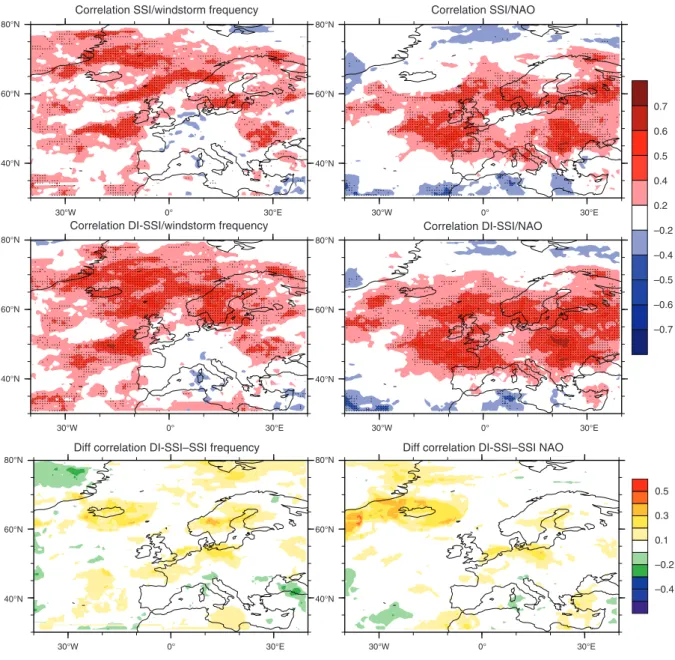
Thus, a storm with extreme surface winds over the sea is subject to high DI-SSI values as the DI-SSI is purely based on the singularity of wind speeds without any potential impact consideration. The biggest discrepancy between the respective rankings for the integral values of the storms is observed for storm Martin (4th com- pared with 8th) which is in line with the arguments for storm Klaus. An application of both indices is shown in Figure 2 (left panel) where the correlation of the annual storm intensity (annual sum of all SSI/DI-SSI contributions within a 500 km radius around a grid cell) and the annual storm occurrence per grid cell is pre- sented. Hunter et al. (2016) showed a similar figure (their Figure 4(a)) using the vorticity as a severity metric. The coherent area of significant values over
50°N
45°N
40°N
35°N
30°N
50°N
45°N
40°N
35°N
30°N
50°N
45°N
40°N
35°N
30°N 50°N
45°N
40°N
35°N
30°N
20°W 10°W 0° 10°E 20°W 10°W 0° 10°E
20°W 10°W 0° 10°E
20°W 10°W 0° 10°E
0 0.1 0.2 0.3 0.4 0.5 0.6 0.7 0.8 0.9 1
–0.35 –0.25 –0.15 –0.05 0.1 0.2 0.3 0.4 0 2 4 6 8 10 12 14 16 18 20 22 24 26 28
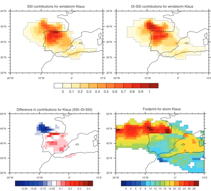
SSI contributions for windstorm Klaus DI-SSI contributions for windstorm Klaus
Difference in contributions for Klaus (SSI–DI-SSI) Footprint for storm Klaus
Figure 3.Footprint of storm Klaus on 24 January 2009 with SSI contributions shown on the top left, the DI-SSI contributions on the top right and the differences between the both values on the bottom left. The footprint of maximum wind speeds (m s−1) for the entire storm is shown in the bottom right panel. Both SSI and DI-SSI were standardized for comparison reasons. Positive values indicate grid cells with larger SSI contributions value; negative values indicate larger DI-SSI contributions. There is a distinct separation represented by the coast line of the northern and western coast of the Iberian Peninsula.
Scandinavia is smaller compared with their results. The overall pattern looks fairly similar though, with most of Scandinavia showing positive correlations, implying that seasons with more storms also feature more intense storms.
Especially for the DI-SSI (middle-left panel), there is a large area of significant correlation between occur- rence and intensity southwest of the British Isles that is not visible in their figure. This indicates the enhanced capability of the DI-SSI to characterize intense and unusual wind speeds not only over land but also over the sea compared with using vorticity as a severity metric.
This is in line with the large DI-SSI value for windstorm Vivian for the DI-SSI is capable of quantifying extreme surface winds regardless of their occurrence. This is also supported by the difference between the two cor- relations shown in the bottom-left panel of Figure 2 as most areas over the Central Atlantic are positive, thus denoting larger DI-SSI correlations.
3.1. SSI and DI-SSI compared for a European storm example
Figure 3 serves as an example of how the previously discussed differences between the SSI and the DI-SSI arise: The figure shows a snapshot of the footprint of storm Klaus (Liberato et al., 2011) and the foot- print of the entire storm in the bottom right panel. The overall footprint of the storm looks exactly the same by definition as the local 98th percentile is used as a detection criterion in the storm tracking algorithm. The geographical intensity distribution however is different for the two indices (both indices are standardized for comparison). Whereas the SSI has its largest contri- butions over land on the northern coast of the Iberian Peninsula, the DI-SSI has in fact its largest contribu- tions over the sea just north of the northern coast of Spain. This area coincides with the area of the most extreme wind speeds. This difference becomes more
obvious when looking at the differences of the contribu- tions of both indices. The coast line of the Iberian Penin- sula represents an almost perfect segregation between negative and positive differences. This is according to the expectation regarding the features of the SSI and DI-SSI. The SSI can be used well to assess the poten- tial damage to infrastructure, however judging from this figure it would seem that the wind speeds over the Atlantic do not have the same exceedance proba- bility as they have over land. The DI-SSI draws a dif- ferent picture: Albeit still showing large values over land, the more extreme values are apparent over the ocean indicating that the wind speeds in that area were even more exceptional with regard to their climatolog- ical wind speed distribution. This supports the argu- ments regarding the large DI-SSI for the storm Vivian in Section 3.
3.2. Intensity indices in connection with the NAO A more quantitative comparison is supplied in the right panel of Figure 2. These two figures show the correla- tion coefficients between the annual winter NAO time series and the annual intensity time series per grid cell for the SSI and DI-SSI, respectively. Grid cells with a correlation coefficient significantly different from zero at the 5% level are stippled. This correlation does not necessarily prove any physical evidence; however, it indicates that the correlation was unlikely if the null hypothesis was true. Considering this fact, both maps show a significant link between the NAO and the inten- sity of European windstorms for most of Europe. How- ever, overall there are more significant grid cells for the correlation using the DI-SSI compared with the SSI. This applies especially to large parts of south- west France, parts of Northern Africa and some areas in northeast Europe, thus regions which are affected less frequently by large scale windstorms. The largest dif- ference in correlation is observed south of Greenland and around Iceland. According to the bottom panel of Figure 1, these areas are also on the edge of the storm track. This is another indication showing that the DI-SSI is a suitable metric to quantify extreme wind speeds out- side the main storm track. The correlation pattern within the main storm track (central North Atlantic) is almost equal for both indices This supports the expectation that they behave fairly similar given the amount of storms per grid cell is sufficiently large.. Thus, the DI-SSI is a useful metric to represent the extremeness of wind speeds both in areas with little annual storm activity and also in areas with increased storminess.
4. Summary and discussion
This study introduces the DI-SSI: It serves as a quan- tification of exceptional surface wind speeds, especially for those high wind speeds occurring outside of the main storm tracks. Due to strongly diverse wind clima- tologies in different regions, the actual wind speed is an
improper metric for the assessment of extremeness. A widely used index, especially in the impact community is the SSI developed by Leckebuschet al.(2008). The SSI is a metric that relates extreme winds to their poten- tial damage on housing or infrastructure, whereas the newly introduced DI-SSI assesses the severity of excep- tional wind speeds based on their occurrence proba- bility: The shape of the tail of the local wind clima- tology is taken into account and used as input regard- ing the objective severity of an event. Thus, the sever- ity of storms occurring within the main storm track can be compared more accurately to those rarer events, e.g. in the Mediterranean area. SSI/DI-SSI values are presented for nine prominent European winter storms.
These values reveal the difference between the two indices. The largest SSI values arise for storms occur- ring on the edges of the storm track (Klaus, Martin), whereas the DI-SSI ranks storm Vivian and Kyrill as the most severe events.
In connection with the NAO index, the DI-SSI time series shows a more coherent area of significant corre- lation over Southwest Europe and also the Baltic Sea area compared with the SSI. This proves the capability of the DI-SSI to assess the severity of extreme winds both inside and outside of the main storm track. A larger area of correlation is also apparent for the cor- relation between frequency and intensity. The overall pattern of correlation for both indices is in agreement with Hunteret al.(2016). The results imply that espe- cially within the main storm track in the North Atlantic and for most parts of Scandinavia, seasons with many storms also tend to feature more intense storms. This is in accordance with Vitolo et al. (2009) who found that serially clustered seasons are likely to spawn more intense storms. Technically, the SSI is easier to com- pute than the DI-SSI for it only requires wind speed data on grid cell level and no fitting of a statistical model.
The DI-SSI requires more processing of the data, how- ever it is a useful additional tool to assess the severity of storms/extreme winds regardless of their geographic occurrence.
Acknowledgements
M.A. Walz has been supported by a National Environmen- tal Research Council (NERC) CENTA PhD scholarship kindly funded by Research Councils UK (RCUK). Fragments of this manuscript were prepared as part of a MSc Thesis at Freie Universität Berlin. H. W. Rust received support by the Freie Universität Berlin within the Excellence Initiative of the Ger- man Research Foundation. G.C. Leckebusch is supported for his research by the European Union (EU) FP7-MC-CIG-322208 grant. The authors thank the ECMWF for providing ERA Interim reanalysis data. The authors would also like to thank Ben Young- man and an anonymous reviewer for many helpful comments.
Supporting information
The following supporting information is available:
Figure S1.Footprint of maximum wind speed for storm Vivian and Kyrill. The very extreme wind speeds over the Central Atlantic Ocean for Vivian are responsible for the very large DI-SSI value compared to all the other storms which are com- pared in Table 2. This is due to the fact that the DI-SSI shows the same magnitude for wind speeds of the same extremeness.
References
Coles SG. 2001.An Introduction to Statistical Modeling of Extreme Values, (Vol. 208). Springer: London.
Cooley D, Nychka D, Naveau P. 2007. Bayesian spatial modeling of extreme precipitation return levels.Journal of the American Statistical Association102(479): 824–840.
Dee D, Uppala S, Simmons A, Berrisford P, Poli P, Kobayashi S, Andrae U, Balmaseda M, Balsamo G, Bauer P. 2011. The ERA-Interim reanalysis: configuration and performance of the data assimilation sys- tem.Quarterly Journal of the Royal Meteorological Society137(656):
553–597.
Donat MG, Leckebusch GC, Pinto JG, Ulbrich U. 2010. Examination of wind storms over Central Europe with respect to circulation weather types and NAO phases.International Journal of Climatology30(9):
1289–1300.
Donat MG, Pardowitz T, Leckebusch GC, Ulbrich U, Burghoff O. 2011.
High-resolution refinement of a storm loss model and estimation of return periods of loss-intensive storms over Germany. Natural Hazards and Earth System Sciences11(10): 2821–2833.
Fink AH, Brücher T, Ermert V, Krüger A, Pinto JG. 2009. The European storm Kyrill in January 2007: synoptic evolution, meteorological impacts and some considerations with respect to climate change.
Natural Hazards and Earth System Sciences9(2): 405–423.
Heffernan J, Stephenson A. 2015. Ismev: R package version 1.40, viewed.
Held H, Gerstengarbe F-W, Pardowitz T, Pinto J, Ulbrich U, Born K, Donat M, Karremann M, Leckebusch G, Ludwig P, Nissen K, Österle H, Prahl B, Werner P, Befort D, Burghoff O. 2013. Projections of global warming-induced impacts on winter storm losses in the German private household sector.Climatic Change121(2): 195–207.
Heming J. 1990. The impact of surface and radiosonde observations from two Atlantic ships on a numerical weather prediction model forecast for the storm of 25 January 1990.Meteorological Magazine 119(1421): 249–259.
Hodges KI, Lee R, Bengtsson L. 2011. A comparison of extratropical cyclones in recent reanalyses ERA-Interim, NASA MERRA, NCEP CFSR, and JRA-25.Journal of Climate24(18): 4888–4906.
Hunter A, Stephenson DB, Economou T, Holland M, Cook I. 2016. New perspectives on the collective risk of extratropical cyclones.Quarterly Journal of the Royal Meteorological Society142(694): 243–256.
Klawa M, Ulbrich U. 2003. A model for the estimation of storm losses and the identification of severe winter storms in Germany.Natural Hazards and Earth System Sciences3(6): 725–732.
Kruschke T. 2015. Winter wind storms: Identification, verification of decadal predictions, and regionalization. Dissertation, Freie Univer- sität Berlin, Berlin, Germany.
Kunz M, Mohr S, Rauthe M, Lux R, Kottmeier C. 2010. Assessment of extreme wind speeds from Regional Climate Models – Part 1:
estimation of return values and their evaluation.Natural Hazards and Earth System Sciences10(4): 907–922.
Leckebusch GC, Renggli D, Ulbrich U. 2008. Development and applica- tion of an objective storm severity measure for the Northeast Atlantic region.Meteorologische Zeitschrift17(5): 575–587.
Liberato ML, Pinto JG, Trigo IF, Trigo RM. 2011. Klaus – an excep- tional winter storm over northern Iberia and southern France.Weather 66(12): 330–334.
Lloyd-Hughes B, Saunders MA. 2002. A drought climatology for Europe.International Journal of Climatology22(13): 1571–1592.
Lumbroso D, Vinet F. 2011. A comparison of the causes, effects and aftermaths of the coastal flooding of England in 1953 and France in 2010.Natural Hazards and Earth System Sciences11(8):
2321–2333.
McCallum E, Norris W. 1990. The storms of January and February 1990.
Meteorological Magazine119(1419): 201–210.
Osinski R, Lorenz P, Kruschke T, Voigt M, Ulbrich U, Leckebusch G, Faust E, Hofherr T, Majewski D. 2016. An approach to build an event set of European windstorms based on ECMWF EPS.Natural Hazards and Earth System Sciences16(1): 255–268.
Palutikof J, Skellern A. 1991. Storm Severity over Britain. A Report to Commercial Union General Insurance, Climatic Research Unit, School of Environmental Sciences, University of East Anglia, Nor- wich (UK).
Parton G, Vaughan G, Norton E, Browning K, Clark P. 2009. Wind profiler observations of a sting jet.Quarterly Journal of the Royal Meteorological Society135(640): 663–680.
Pinto JG, Zacharias S, Fink AH, Leckebusch GC, Ulbrich U. 2009.
Factors contributing to the development of extreme North Atlantic cyclones and their relationship with the NAO. Climate Dynamics 32(5): 711–737.
SwissRe. 2016. Natural Catastrophes and Man-Made Disasters in 2015:
Asia suffers substantial losses. Sigma No 1/2016. Order number:
270_0116_EN.
Tripoli G, Medaglia C, Dietrich S, Mugnai A. 2005. The 9–10 November 2001 Algerian flood.Bulletin of the American Meteorological Society 86(9): 1229.
Ulbrich U, Christoph M. 1999. A shift of the NAO and increasing storm track activity over Europe due to anthropogenic greenhouse gas forcing.Climate Dynamics15(7): 551–559.
Ulbrich U, Fink A, Klawa M, Pinto J. 2001. Three extreme storms over Europe in December 1999.Weather56(3): 70–80.
Vitolo R, Stephenson DB, Cook IM, Mitchell-Wallace K. 2009. Serial clustering of intense European storms.Meteorologische Zeitschrift 18(4): 411–424.
Vrac M, Naveau P. 2007. Stochastic downscaling of precipitation:
from dry events to heavy rainfalls.Water Resources Research43(7):
W07402.