Improving Smartphone-Based GNSS Positioning Using State Space Augmentation Techniques

Veröffentlichungen der DGK

Ausschuss Geodäsie der Bayerischen Akademie der Wissenschaften

Reihe C Dissertationen Heft Nr. 864

Francesco Darugna

Improving Smartphone-Based GNSS Positioning Using State Space Augmentation Techniques

München 2021

Verlag der Bayerischen Akademie der Wissenschaften

ISSN 0065-5325 ISBN 978-3-7696-5276-5

Diese Arbeit ist gleichzeitig veröffentlicht in:

Wissenschaftliche Arbeiten der Fachrichtung Geodäsie und Geoinformatik der Universität Hannover ISSN 0174-1454, Nr. 368, Hannover 2021

Veröffentlichungen der DGK

Ausschuss Geodäsie der Bayerischen Akademie der Wissenschaften

Reihe C Dissertationen Heft Nr. 864

Improving Smartphone-Based GNSS Positioning Using State Space Augmentation Techniques

Von der Fakultät für Bauingenieurwesen und Geodäsie der Gottfried Wilhelm Leibniz Universität Hannover

zur Erlangung des Grades Doktor-Ingenieur (Dr.-Ing.) genehmigte Dissertation

Vorgelegt von

M. Sc. Francesco Darugna

Geboren am 21.01.1992 in Feltre, Italy

München 2021

Verlag der Bayerischen Akademie der Wissenschaften

ISSN 0065-5325 ISBN 978-3-7696-5276-5

Diese Arbeit ist gleichzeitig veröffentlicht in:

Wissenschaftliche Arbeiten der Fachrichtung Geodäsie und Geoinformatik der Universität Hannover ISSN 0174-1454, Nr. 368, Hannover 2021

Adresse der DGK:

Ausschuss Geodäsie der Bayerischen Akademie der Wissenschaften (DGK)

Telefon +49 – 331 – 288 1685 ● Telefax +49 – 331 – 288 1759 E-Mail post@dgk.badw.de ● http://www.dgk.badw.de

Prüfungskommission:

Vorsitzender: Prof. Dr.-Ing. habil. Christian Heipke Referent: Prof. Dr.-Ing. Steffen Schön

Korreferenten: Prof. Dr. Fabio Dovis (Politecnico di Torino) Prof. Dr.-Ing. habil. Monika Sester Tag der mündlichen Prüfung: 18.11.2020

© 2021 Bayerische Akademie der Wissenschaften, München

Alle Rechte vorbehalten. Ohne Genehmigung der Herausgeber ist es auch nicht gestattet,

die Veröffentlichung oder Teile daraus auf photomechanischem Wege (Photokopie, Mikrokopie) zu vervielfältigen

ISSN 0065-5325 ISBN 978-3-7696-5276-5

A ^BSTRACT

Low-cost receivers providing Global Navigation Satellite System (GNSS) pseudorange and car- rier phase raw measurements for multiple frequencies and multiple GNSS constellations have become available on the market in the last years. This significantly has increased the number of devices equipped with the necessary sensors to perform precise GNSS positioning. GNSS pseudorange and carrier phase are used to compute user positions. While both observations are affected by different error sources, e.g. the passage through the atmosphere, only the carrier-phase has an ambiguous nature. The resolution of this ambiguity is a crucial factor to reach fast and highly precise GNSS-based positioning.

Currently, several smartphones are equipped with a dual-frequency, multi-constellation receiver. The access to Android-based GNSS raw measurements has become a strong motiva- tion to investigate the feasibility of smartphone-based high-accuracy positioning. The quality of smartphone GNSS measurements has been analyzed, suggesting that they often suffer from low signal-to-noise, inhomogeneous antenna gain and high levels of multipath. This work shows how to tackle several of the currently present obstacles and demonstrates centimeter- level positioning with a low-cost GNSS antenna and a low-cost GNSS receiver built into an off-the-shelf smartphone.

Since the beginning of the research in smartphone-based positioning, the device’s GNSS antenna has been recognized as one of the main limitations. Besides Multipath (MP), the an- tenna radiation pattern is the main site-dependent error source of GNSS observations. An absolute antenna calibration has been performed for the dual-frequency smartphone Huawei Mate20X. Antenna Phase Center Offset (PCO), and Variations (PCV) have been estimated to correct for the antenna impact on the L1 and L5 phase observations. Accordingly, the rele- vance of considering the individual PCO and PCV for the two frequencies is shown. The PCV patterns indicate absolute values up to 2 cm and 4 cm for L1 and L5, respectively. The impact of antenna corrections has been assessed in different multipath environments using a high- accuracy positioning algorithm employing an uncombined observation model and applying Ambiguity Resolution (AR). Experiments both in zero-baseline and short-baseline configura- tions have been performed. Instantaneous AR in the zero-baseline setup has been demon- strated, showing the potential for cm-level positioning with low-cost sensors available inside smartphones. In short-baselines configurations, no reliable AR is achieved without antenna corrections. However, after correcting for PCV, successful AR is demonstrated for a smartphone placed in a low multipath environment on the ground of a soccer field. For a rooftop open-sky test case with large multipath, AR was successful in 19 out of 35 data-sets. Overall, the an- tenna calibration is demonstrated being an asset for smartphone-based positioning with AR, showing cm-level 2D Root Mean Square Error (RMSE).

In GNSS-based positioning, a user within a region covered by a network of reference sta-

tions can take advantage of the network-estimated augmentation parameters. Among the

GNSS error sources, atmospheric delays have a strong impact on the positioning performance

and the ability to resolve ambiguities. State Space Representation (SSR) atmospheric cor-

rections, i.e. tropospheric and ionospheric delays, are commonly estimated for the approx-

imate user position by interpolation from values calculated for the reference stations. Widely

used interpolation techniques are Inverse Distance Weighted (IDW), Ordinary Kriging (OK)

and Weighted Least Squares (WLS). The interpolation quality of such techniques during se-

vere weather events and Traveling Ionospheric Disturbances (TIDs) is analyzed. To improve

the interpolation performance during such events, modified WLS methods taking advantage

of the physical atmospheric behavior are proposed. To support this interpolation approach, external information from Numerical Weather Models (NWM) for tropospheric interpolation and from TID modeling for ionospheric interpolation is introduced to the algorithms.

The interpolation is assessed using simulated data (considering artificial and real network geometries), and real SSR parameters generated by network computation of GNSS measure- ments. As examples, two severe weather events in northern Europe in 2017 and one TID event over Japan in 2019 have been analyzed. The interpolation of SSR Zenith Tropospheric Delay (ZTD) and ionospheric parameters is evaluated. Considering the reference station positions as rover locations, the modified WLS approach marks a lower RMSE in up to 80% of the cases during sharp weather fluctuations. Also, the average error can be decreased in 64% of the cases during the TID event investigated. Improvements up to factors larger than two are observed.

Furthermore, specific cases are isolated, showing particular ZTD variations where significant errors (e.g. larger than 1 cm) can be reduced by up to 20% of the total amount. As a final product of the analysis, tropospheric and ionospheric messages are proposed. The messages contain the information needed to implement the suggested interpolation.

Along with the need for accurate atmospheric models, the concept of consistency in the SSR corrections is crucial. A format that can transport all the SSR corrections estimated by a network is the Geo++ SSR format (SSRZ). Exploiting the features of the SSRZ format, the impact of an error in the transported ionospheric parameters is investigated. It is shown that the position estimation strongly depends on the ionospheric modeling and mismodeling can result in cm level errors, especially in the height component.

Keywords: SSR, GNSS smartphone-based positioning, GNSS antenna calibration, atmo-

spheric interpolation

K ^URZFASSUNG

In den letzten Jahren sind kostengünstige Empfänger auf dem Markt verfügbar geworden, die Pseudorange- und Trägerphasenrohmessungen für mehrere Frequenzen und mehrere Kon- stellationen der Global Navigation Satellite Systems (GNSS) ermöglichen. Dies erhöht die An- zahl der Geräte, die mit den erforderlichen Sensoren ausgestattet sind, um eine präzise GNSS- Positionierung durchzuführen, erheblich. GNSS-Pseudorange- und Trägerphasenbeobach- tungen werden verwendet, um Benutzerpositionen zu berechnen. Während beide Beobach- tungen von unterschiedlichen Fehlerquellen beeinflusst werden, z.B. beim Durchgang durch die Atmosphäre, ist nur die der Trägerphase mehrdeutig. Die Auflösung dieser Mehrdeutigkeit ist ein entscheidender Faktor für eine schnelle und hochpräzise GNSS-basierte Positionierung.

Derzeit sind einige Smartphones mit einem Zwei-Frequenz-Multi-GNSS-Empfänger ausges- tattet. Der Zugriff auf Android-basierte GNSS-Rohmessungen ist zu einer starken Motivation geworden, die Smartphone-basierten Positionierung zu untersuchen.

Die Ergebnisse der Qualitätsanalyse von GNSS-Messungen mit Smartphones deuten darauf hin, dass Smartphone-Beobachtungen häufig durch ein geringes Signal-Rausch- Verhältnis, einer inhomogenen Antennencharakteristik und einem hohen Mehrwegepegel (Multipath-Effekte) beeinträchtigt sind. Diese Arbeit zeigt, wie mehrere der derzeit vorhan- denen Hindernisse überwunden werden können und die Positionierung mit Zentime- tergenauigkeit mit einer kostengünstigen GNSS-Antenne und einem kostengünstigen GNSS-Empfänger in einem handelsüblichen Smartphone erreicht wird. Schon zu Beginn der Forschung wurde die GNSS-Antenne des Smartphone als eine der größten Fehlerquellen in der Positionierung erkannt, wobei neben Multipath (MP) die Empfangscharakteristik der Antenne die wichtigste ortsabhängige Fehlerquelle für GNSS-Beobachtungen darstellt. In dieser Arbeit werden Ergebnisse der absoluten Antennenkalibrierung des Zwei-Frequenz-Huawei Mate20X vorgestellt. Für das Zwei-Frequenz-Huawei Mate20X wurde eine absolute Antennenkalib- rierung durchgeführt und der Phase-Center-Offset (PCO) und die Phase-Center-Variations (PCV) geschätzt, um den Einfluss der Antenne auf die Phasenbeobachtungen von L1 und L5 zu korrigieren. Die Relevanz dieser beiden Korrekturen wird für die beiden Frequenzen gezeigt.

Die PCV-Werte variieren um bis zu 2cm für L1 und um bis zu 4cm für L5. Die Auswirkungen von Antennenkorrekturen wurden in verschiedenen Mehrwegeumgebungen mithilfe eines hochgenauen Positionierungsalgorithmus unter Verwendung der Mehrdeutigkeitslösung (Ambiguity Resolution AR) für die zwei Phasenbeobachtungen untersucht.

Es wurden Experimente sowohl in Nullbasislinien- als auch in Kurzbasislinien-

Konfigurationen durchgeführt. Dabei konnte eine sofortige Mehrdeutigkeitsauflösung im

Nullbasislinien-Setup demonstriert werden, die das Potenzial für die Positionierung auf Zen-

timetergenauigkeit mit kostengünstigen Smartphone-Sensoren zeigt. In Konfigurationen mit

kurzen Basislinien wird ohne Antennenkorrekturen keine zuverlässige Mehrdeutigkeitsauflö-

sung erreicht. Mit der Anbringung der PCV-Korrektur an die Smartphone-Antenne wird jedoch

eine erfolgreiche Auflösung für ein Smartphone demonstriert, das sich in einer Umgebung

mit geringem Mehrwegeffekt auf dem Boden eines Fußballfelds befindet. Für einen Open-

Sky-Testfall auf dem Dach mit starken Mehrwegeeffekt war die Mehrdeutigkeitsauflösung in

19 von 35 Datensätzen erfolgreich. Diese Analysen zeigen, dass die Antennenkalibrierung

ein Vorteil für die Smartphone-basierte Positionierung mit Mehrdeutigkeitsauflösung ist und

der 2D RMS-Fehler (RMSE) im Zentimeterbereich erreicht werden kann. Die Mehrdeutigkeit-

sauflösung und damit die Positionierungsperformance werden stark durch atmosphärische

Effekte beeinflusst. Befindet sich ein GNSS-Nutzer innerhalb einer Region, die von einem

Referenzstationsnetzwerk abgedeckt wird, kann dieser die mit dem Netzwerk ermittelten Korrekturdaten nutzen. Die State Space Representation (SSR) stellt u.a. atmosphärische Korrekturen bereit, die der Nutzer für seine ungefähre Position individualisieren kann.

Für die Individualisierung werden verschiedene Interpolationsmethoden benutzt. Weit verbreitete Interpolationstechniken sind die Inverse Distance Weighted (IDW), Ordinary Kriging (OK) und Weighted Least Squares (WLS) Methode. Die Qualität dieser Interpolation- smethoden bei Unwetterereignissen und Traveling Ionospheric Disturbances (TIDs) wird analysiert. Um die Interpolationsleistung während solcher Ereignisse zu verbessern, werden modifizierte WLS-Verfahren vorgeschlagen, die das physikalische Atmosphärenverhalten ausnutzen. Um diesen Interpolationsansatz zu unterstützen, werden externe Informationen aus numerischen Wettermodellen (NWM) für die troposphärische Interpolation und aus der TID-Modellierung für die ionosphärische Interpolation in die Algorithmen eingeführt. Die Bewertung der Interpolationenverfahren basiert einerseits auf der Verwendung simulierter Daten in künstlichen und realen Netzwerkgeometrien und anderseits auf der Verwendung realer SSR-Parameter, die während zweier Unwetterereignisse in Nordeuropa im Jahr 2017 und einem TID-Ereignis über Japan im Jahr 2019 erzeugt wurden. Die Interpolation der SSR-Zenit- Troposphärenverzögerung (ZTD) und der ionosphärischen Parameter werden analysiert.

Unter Verwendung einer Referenzstation als Rover zeigt der modifizierte WLS-Ansatz in bis zu 80 % der Fälle bei starken Wetterschwankungen einen niedrigeren RMSE. Darüber hinaus kann der durchschnittliche Fehler in 64 % der Fälle während des untersuchten TID-Ereignisses verringert werden. Verbesserungen bis zu einem Faktor größer als zwei werden beobachtet.

Darüber hinaus werden solche Fälle isoliert, die bestimmte ZTD-Variationen zeigen, bei denen signifikante Fehler (z.B. größer als 1 cm) auf bis zu 20 % der Gesamtmenge reduziert werden können. Für die Anwendung der modifizierten Interpolationen in der Praxis werden Nachrichten(formate) vorgeschlagen, die die erforderlichen Informationen für die ordnungs- gemäße Implementierung der vorgeschlagenen ionosphärischen und troposphärischen Interpolationen beinhalten. Neben der Notwendigkeit genauer atmosphärischer Modelle ist das Konzept der Konsistenz bei den SSR-Korrekturen von entscheidender Bedeutung. Ein Format, das alle von einem Netzwerk geschätzten SSR-Korrekturen transportieren kann, ist das Geo++ SSR-Format SSRZ. Unter Ausnutzung der Merkmale des SSRZ-Formats wird die Auswirkung eines Fehlers in den transportierten ionosphärischen Parametern untersucht.

Es wird gezeigt, dass die Positionsschätzung stark von der ionosphärischen Modellierung abhängt und eine Fehlmodellierung zu Fehlern auf Zentimeterniveau insbesondere in der Höhenkomponente führen können.

Schlagwörter: SSR, GNSS-Smartphone-basierte Positionierung, GNSS-Antennenkalibrierung,

atmosphärische Interpolation

A ^CRONYMS

A-GNSS Assisted-GNSS

ADR Accumulated Delta Range AR Ambiguity Resolution

BDS BeiDou Navigation Satellite System

BKG Federal Agency for Cartography and Geodesy

BN BiasNanos

C/N0 Carrier to Noise density ratio CNES National Centre for Space Studiess

CORS Continuously Operation Reference Stations

CT Clough Tocher

DD Double Difference DLL Delay Lock Loop

DLR German Aerospace Center ECEF Earth-Centered Earth-Fixed

ECMWF European Center for Medium-Range Weather Forecasts ESA European Space Agency

ETH Eidgenössische Technische Hochschule FBN FullBiasNanos

FKP Flaechen Korrektur Parameter GDOP Geometric Dilution of Precision GDV Group Delay Variations

GEONET GNSS Earth Observation Network System GFS Global Forecasting System

GFZ German Research Centre for Geosciences GIM Global Ionospheric propagation Model

GLONASS GLObal’naya Navigatsionnaya Sputnikovaya Sistema

GNSMART GNSS State Monitoring and Representation Technique

GNSS Global Navigation Satellite System

GPO Ground Point Origin GPS Global Positioning System

GREF Integrated Geodetic Reference Network of Germany

GT GPS Time

GVI Global Vertical Ionosphere GRI Gridded Ionosphere GRT Gridded Troposphere

GSI Global Satellite-dependent Ionosphere HDOP Horizontal Dilution of Precision IDW Inverse Distance Weighted IF Intermediate Frequency IGS International GNSS Service IGS RTS IGS Real-Time Service IPA Initial Phase Ambiguity IPB Initial Phase Bias

IPP Ionospheric Pierce Point

IRI International Reference Ionosphere

IRNSS Indian Regional Navigation Satellite System ISB Inter-System Biases

ITRF International Terrestrial Reference Frame JPL Jet Propulsion Laboratory

LAMBDA Least-squares AMBiguity Decorrelation Adjustment

LGLN-SAPOS Landesamt für Geoinformation und Landesvermessung Niedersachsen - Satellitenpositionierungsdienst

LS Least Squares

OSR Observation Space Representation MAC Master-Auxiliary-Concept

Mate20X Huawei Mate20X

Mi8 Xiaomi Mi8

MP Multipath

MSTID Medium-Scale TID

NCO Numerically Controlled Oscillator

NRCan Natural Resources Canada NRP North Reference Point N-RTK Network-RTK

NTRIP Networked Transport of RTCM via Internet Protocol OK Ordinary Kriging

PC electrical mean Phase Center PCB Printed Circuit Board

PCC Phase Center Corrections PCO Phase Center Offset PCV Phase Center Variations PDOP Position Dilution of Precision PLL Phase Lock Loop

POD Precise Orbit Determination PPO Pierce Point Origin

PPP Precise Point Positioning

PPP-RTK Precise Point Positioning - Real-Time Kinematic QZSS Quasi Zenith Satellite System

RF Radio Frequency

RIU Residual Interpolation Uncertainty RMSE Root Mean Square Error

RSI Regional Satellite-dependent Ionosphere RT Regional Troposphere

RTCM Radio Technical Commission for Maritime Services RTK Real-Time Kinematic

SC Special Committee SMA SubMiniature version A SoC System on Chip

SPP Single Point Positioning

SSM State Space Modeling

SSR State Space Representation

STD Standard deviation

STEC Slant Total Electron Content TEC Total Electron Content TECU Total Electron Content Unit TID Traveling Ionospheric Disturbance TOD Time Of the Day

TOW Time Of the Week

TREASURE Training REsearch and Applications Network to Support the Ultimate Real-Time High Accuracy EGNSS Solution

TTFA Time To Fix Ambiguities TTSM Time To achieve Sub-Meter VDOP Vertical Dilution of Precision VGMF Vienna Global Mapping Functions VTEC Vertical Total Electron Content WLS Weighted Least Squares WGS84 World Geodetic System 1984 WHU Wuhan University

ZHD Zenith Hydrostatic Delay

ZTD Zenith Tropospheric Delay

ZWD Zenith Wet Delay

1 Introduction 1

2 GNSS Positioning Techniques 7

2.1 The GNSS observation equations . . . . 7

2.1.1 Pseudorange measurements . . . . 8

2.1.2 Carrier phase measurements . . . . 9

2.1.3 Atmospheric delays . . . . 9

2.1.4 Double-Difference (DD) observations . . . . 12

2.2 GNSS augmentation techniques . . . . 14

2.2.1 State Space Modeling (SSM) . . . . 14

2.2.2 State Space Representation (SSR) . . . . 15

2.2.3 SSR corrections . . . . 16

2.2.4 Observation Space Representation (OSR) . . . . 21

2.3 RTK positioning . . . . 22

2.4 Positioning with uncombined observation model . . . . 23

3 Smartphone-Based Positioning 25 3.1 Motivation . . . . 25

3.2 The construction of the observations . . . . 26

3.2.1 Pseudorange calculation . . . . 27

3.2.2 Phase observation computation . . . . 29

3.2.3 Continuity of phase measurements . . . . 30

3.3 Quality analysis of smartphone measurements . . . . 32

3.3.1 Setup . . . . 32

3.3.2 Phase double-difference analysis . . . . 34

3.3.3 Code noise and multipath investigation . . . . 44

3.3.4 Allan deviation analysis . . . . 49

3.3.5 Expected positioning performance . . . . 50

3.3.6 Smartphone-based ionospheric TEC measurements . . . . 51

3.4 Positioning using smartphones . . . . 52

3.4.1 Zero and short-baselines applications . . . . 53

3.4.2 Network SSR-based positioning . . . . 58

3.4.3 SPP and PPP using smartphone’s observations . . . . 60

3.5 Discussion . . . . 60

4 PCV Impact on Smartphone-Based Positioning 63 4.1 Motivation . . . . 63

4.2 Absolute robot-based field calibration of GNSS antennas . . . . 64

4.3 The Huawei Mate20X antenna calibration . . . . 66

4.3.1 Analysis of the Mate20X’s PCV . . . . 66

4.3.2 PCV repeatability . . . . 71

4.3.3 Smartphone antenna location . . . . 75

4.4 High-accuracy smartphone-based positioning . . . . 78

4.4.1 Positioning in Scenario 4: the soccer field test . . . . 79

4.4.2 Positioning in Scenario 3: the rooftop test . . . . 84

Contents

4.5 Discussion . . . . 89

5 Mitigating the Impact of SSR Atmospheric Parameter Errors 91 5.1 Motivation . . . . 91

5.2 Expected impact on positioning . . . . 93

5.3 Interpolation techniques . . . . 94

5.3.1 Interpolation of scattered data . . . . 94

5.3.2 Methods introduction . . . . 95

5.3.3 Modified WLS methods . . . . 97

5.4 Interpolation of simulated data . . . . 98

5.4.1 Simulation setup . . . . 98

5.4.2 Generation of error patterns . . . 100

5.4.3 Results for artificial grids . . . 100

5.4.4 Results for real-network geometries . . . 102

5.4.5 Required precision for the directional information . . . 104

5.4.6 Variation of the interpolation position . . . 105

5.4.7 Variation of the distance: WLS methods comparison . . . 106

5.5 ZTD interpolation during severe weather events . . . 108

5.5.1 Data-sets and analysis concept . . . 108

5.5.2 Comparison of NWM gradients and spatial distribution of GNSS- estimated ZTD . . . 112

5.5.3 Interpolation results using directional techniques . . . 113

5.5.4 Impact of test location . . . 115

5.6 Interpolation of residual ionospheric effects during a TID . . . 117

5.6.1 Data-set and extraction of TID event . . . 117

5.6.2 Improved interpolation strategy . . . 119

5.7 Error propagation: from SSR modeling to the user . . . 121

5.7.1 Ambiguity resolution with ionospheric biases: simulation . . . 121

5.7.2 Real-time impact on positioning of an ionospheric SSR error . . . 122

5.8 Discussion . . . 125

6 Conclusions and outlook 129 A RTCM-SSR Python demo 131 B SSRZ Python demo 141 C Smartphone-based positioning: additional information 149 C.1 Phase DD in Scenario 1: specific satellite examples . . . 149

C.2 Smartphone-based positioning using GNSMART . . . 149

C.3 GNSS raw measurements: Android API classes . . . 150

1.1 Representation of range and SSR corrections . . . . 2

1.2 Outline of the thesis . . . . 4

3.1 Time reconstruction from GNSS raw measurements: GPS example . . . . 29

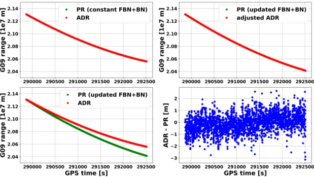
3.2 Comparison of ADR computed from Android API with constant and updated FBN 31 3.3 Geo++ GmbH rooftop and zero-baseline setup between smartphone and geode- tic receiver. . . . 33

3.4 Smartphone on soccer field experiment setup. . . . 34

3.5 Phase DD in zero-baseline setup with smartphone in RF enclosure . . . . 36

3.6 GPS C/N0 and elevation of smartphone measurements in zero-baseline within RF enclosure . . . . 36

3.7 Galileo C/N0 and elevation of smartphone measurements in zero-baseline within RF enclosure . . . . 37

3.8 Example of phase DD jump in smartphone’s measurements . . . . 37

3.9 Phase DD in zero-baseline setup with smartphone in RF enclosure with 13dB attenuation . . . . 38

3.10 GPS C/N0 and elevation of smartphone measurements in zero-baseline within RF enclosure with 13 dB attenuation . . . . 39

3.11 Galileo C/N0 and elevation of smartphone measurements in zero-baseline within RF enclosure with 13 dB attenuation . . . . 39

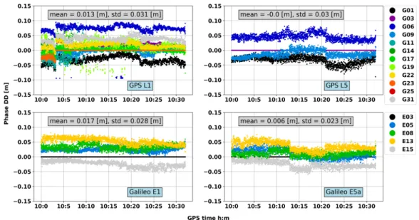
3.12 Phase DD in open sky rooftop . . . . 40

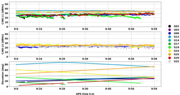
3.13 GPS C/N0 and elevation of smartphone measurements in an open sky rooftop . 41 3.14 Galileo C/N0 and elevation of smartphone measurements in open sky rooftop . 41 3.15 Mean of phase DD absolute values in open sky rooftop . . . . 42

3.16 Phase DD in the soccer field . . . . 42

3.17 GPS C/N0 and elevation of smartphone measurements in the soccer field . . . . 43

3.18 Galileo C/N0 and elevation of smartphone measurements in the soccer field . . . 43

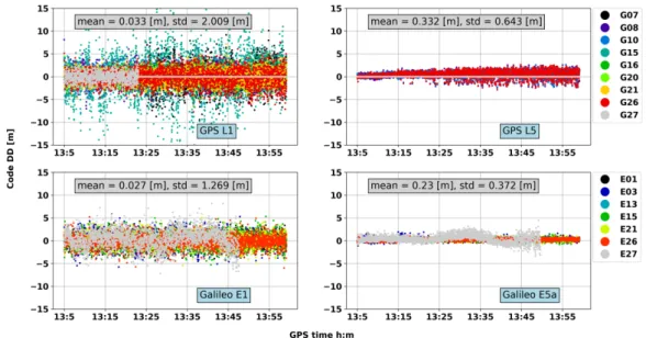
3.19 Code DD in zero-baseline configuration with smartphone within RF enclosure . 44 3.20 Code DD in zero-baseline configuration with smartphone within RF enclosure with 13 dB attenuation . . . . 45

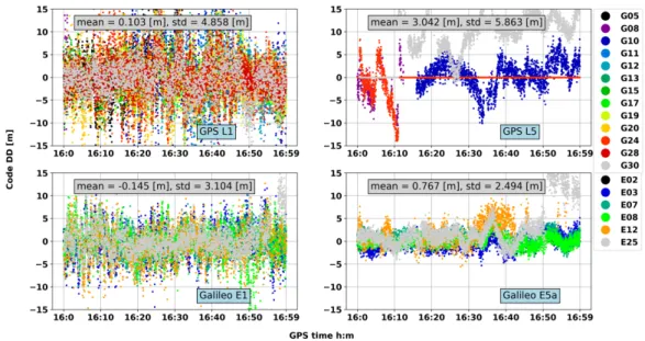
3.21 Code DD in open sky rooftop environment . . . . 45

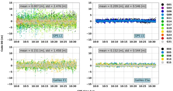
3.22 Code DD in the soccer field . . . . 46

3.23 Multipath in the soccer field. . . . 47

3.24 Setup of multipath-impact experiment: smartphone at different heights. . . . 47

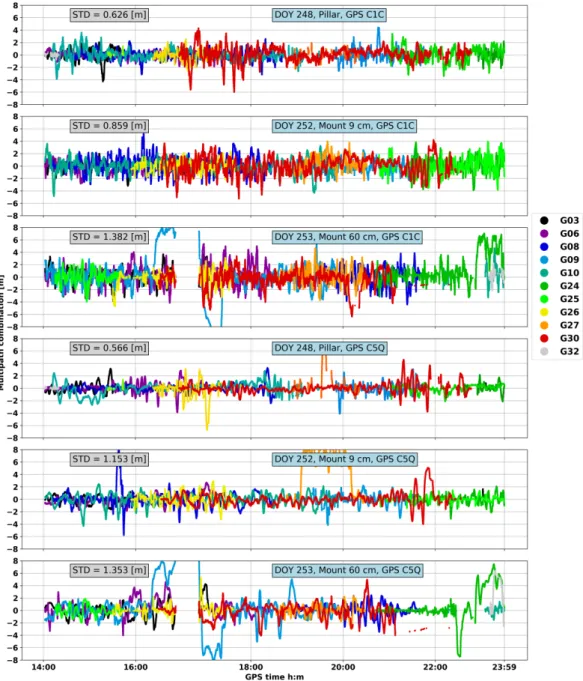
3.25 Moving average of multipath combination: pillar on Geo++ rooftop. . . . 48

3.26 Moving average of multipath combination: G30 example with C/N0 and elevation 49 3.27 Allan deviation of phase DD in Scenario 3 . . . . 50

3.28 Example of Allan deviation versus the exponent of the power law noise process α of phase DD in Scenario 3 . . . . 51

3.29 Smartphone-based positioning: zero-baseline results . . . . 55

3.30 Smartphone-based positioning: short-baseline results . . . . 56

3.31 Smartphone-based positioning: short-baseline results in a soccer field . . . . 56

3.32 Smartphone-based positioning: pillar setups . . . . 57

3.33 Smartphone-based positioning: 2D error of 30h test over a choke-ring . . . . 57

3.34 Smartphone-based positioning: the toy train experiment . . . . 58

List of Figures 3.35 Smartphone-based positioning: sub-set of the LGLN network used to generate

SSR parameters . . . . 59

3.36 Smartphone-based positioning: real-time experiment . . . . 59

3.37 Smartphone-based positioning: network SSR-based in post-processing . . . . 60

4.1 Smartphone antenna calibration: reference frame and estimated phase centers . 65 4.2 Smartphone antenna calibration: setup and concept. . . . 66

4.3 Smartphone antenna calibration: Mate20X antenna PCV. . . . 68

4.4 Smartphone antenna calibration: Mate20X antenna PCV formal STD. . . . 69

4.5 Smartphone antenna calibration: example of PCV geodetic rover antenna . . . . 70

4.6 Smartphone antenna calibration: Mate20X antenna PCV of L0. . . . 71

4.7 Smartphone antenna calibration: example of Mate20X antenna PCV difference w.r.t. type-mean. . . . 72

4.8 Smartphone antenna calibration: STD of Mate20X antenna PCV difference w.r.t. type-mean. . . . 73

4.9 Smartphone antenna calibration: Mate20X antenna PCV repeatability w.r.t. type-mean. . . . 74

4.10 Smartphone antenna calibration: antenna location test . . . . 75

4.11 C/N0 color-map of the L1 reception on the front side of the Mate20X. . . . 76

4.12 C/N0 color-map of the L5 reception on the front side of the Mate20X. . . . 77

4.13 Smartphone antenna calibration: antenna location on the phone shell . . . . 78

4.14 GPS phase DD in the soccer field . . . . 80

4.15 Galileo phase DD in the soccer field . . . . 80

4.16 GPS phase DD with C/N0 mask in the soccer field. . . . 81

4.17 PCV impact on GPS phase DD in the soccer field . . . . 81

4.18 PCV impact on Galileo phase DD in the soccer field . . . . 82

4.19 Mate20X positioning performance in the soccer field . . . . 83

4.20 Positioning performance in the soccer field: Mate20X 50 m from reference sta- tion with 5 min reset. . . . 84

4.21 2D error locating the smartphone on poles over the pillar. . . . 85

4.22 Geo++ GmbH rooftop: pillars considered. . . . 86

4.23 DOP of unsuccessful AR period. . . . 86

4.24 DOP of successful AR period. . . . 87

4.25 Mate20X positioning performance on the Geo++ rooftop: unsuccessful AR. . . . 88

4.26 Mate20X positioning performance on the Geo++ rooftop: successful AR. . . . 88

4.27 Histogram of TFFA on the Geo++ rooftop. . . . 89

5.1 Weight isolines for the WLS methods when using the distance d and the modified distance ˜ d . . . . 98

5.2 Artificial networks built to simulate the interpolation performance . . . . 99

5.3 Real reference stations networks . . . . 99

5.4 Performance of the interpolation techniques in a squared grid network . . . 101

5.5 Performance of the interpolation techniques in a circular grid network . . . 102

5.6 Interpolation techniques performance using simulated data with the geometry of the NETPOS network . . . 103

5.7 Interpolation techniques performance using simulated data with the geometry of the LGLN network . . . 103

5.8 Interpolation techniques performance using simulated data with the geometry of the GEONET network . . . 104

5.9 Sensitivity to the error in the estimation of the direction of propagation of the parameter . . . 105

5.10 Map of the best WLS approach in the NETPOS network using artificial data. . . . 106

5.11 Map of the best WLS approach in the LGLN network using artificial data . . . 107

5.12 Map of the best WLS approach in the GEONET network using artificial data . . . 107

5.13 GNSS-estimated and NWM-based ZTD comparison . . . 109

5.14 GNSS-estimated and NWM-based ZTD comparison . . . 109

5.15 DWD weather data: pressure over temperature . . . 110

5.16 DWD weather data: humidity over temperature squared . . . 111

5.17 DWD weather data: precipitations . . . 111

5.18 Average ZTD values computed from GNSS data and NWM gradients for the NET- POS network . . . 113

5.19 Average ZTD values computed from GNSS data and NWM gradients for the LGLN network . . . 113

5.20 Cumulative interpolation error of ZTD data during weather fluctuations . . . 115

5.21 ZTD distribution along gradient direction and cumulative error during a partic- ularly perturbed hour . . . 116

5.22 TEC values of the ionospheric grid residual SSR parameter for satellite E31 during the TID interval . . . 118

5.23 Comparison between average WLS2 and WLS2DL interpolation error in the Oki- nawa GEONET network . . . 119

5.24 Cumulative interpolation error for the E01, E13, E31 satellites . . . 120

5.25 Cumulative error for satellite E31 . . . 120

5.26 Simulation of ambiguity resolution performance in presence of ionospheric biases.122 5.27 Setup for the evaluation of the impact of ionospheric errors in the SSR messages 123 5.28 LGLN sub-net used in the SSRZ error injection test . . . 123

5.29 SSR-based positioning results comparison with artificial ionospheric error in the SSRZ stream . . . 124

C.1 Specific satellite examples of phase DD in Scenario 1 compared to TD, C/N0 and

elevation . . . 149

List of Figures

3.1 C/N0 scenarios used for the DD test. . . . 34

4.1 Calibration characteristic values of the Mate20X’s PCV . . . . 67

4.2 Smartphone-based positioning results. . . . 89

5.1 Summary of the best and second best interpolation in terms of RMSE in the three real networks . . . 106

5.2 Summary of interpolation results of ZTD estimated using GNSS data from the NETPOS and LGLN networks. . . 114

5.3 Summary of interpolation results of ZTD estimated using GNSS data from the NETPOS and LGLN networks w.r.t. WLS2 method. . . 114

5.4 NWM gradients and TID parameters proposed messages . . . 127

A.1 RTCM-SSR standardized messages (RTCM Special Committee No. 104, 2016). . . 131

A.2 RTCM-SSR proposed messages. . . 132

B.1 Current SSRZ messages (Geo++ GmbH, 2020). . . 141

C.1 Android Location API - GNSSMeasurements constants. . . 150

C.2 Android Location API - Clock and Measurements fields. . . 151

1. Introduction

Currently, the individual localization on a map using portable devices is an everyday activity that almost everybody in the world can experience. The roots of the essential principle behind it can be found in the science of mapping and measuring the Earth’s surface, i.e. the classic def- inition of geodesy given by Helmert (Helmert, 1880-1884). In fact, one of the basic problems that geodesy tackles is the computation of precise global, regional and local three-dimensional positions (Seeber, 2003). However, geodesy science includes many different applications, e.g.

the computation of the terrestrial gravity field and ocean surface modeling. Satellite geodesy uses measurements from artificial satellites orbiting around the Earth to solve geodesy-related problems (Seeber, 2003). The use of artificial satellites implies a good knowledge of the posi- tion of the satellites in their orbital motion around the Earth. It is therefore related to Precise Orbit Determination (POD) studies. The tasks involving satellite geodesy are variegated: e.g., to measure the motion of continents precisely and to monitor global deformation of the Earth.

The satellites that provide such measurements are constellations of satellites, the so-called Global Navigation Satellite Systems (GNSSs). As suggested by the name, these constellations provide global coverage of the Earth, being an asset for geodesy-related purposes.

Since the first complete GNSS constellation, i.e. the Navigation System with Time And Ranging (NAVSTAR) Global Positioning System (GPS), in 1995, in the last decades, many im- pressive results have been achieved and new constellations built. In addition to GPS, GNSS constellations with global coverage are the Russian GLObal’naya Navigatsionnaya Sputniko- vaya Sistema (GLONASS), the European Galileo and the Chinese BeiDou Navigation Satellite System (BDS). Furthermore, there are constellations with regional coverage, the so-called Re- gional Navigation Satellite Systems (RNSS): the Japanese Quasi-Zenith Satellite System (QZSS) and the Indian Regional Navigation Satellite System (IRNSS) renamed to Navigation with In- dian Constellation (NavIC) in 2016. Besides the GNSS/RNSSs, there are also the Satellite-Based Augmentation Systems (SBASs). SBAS constellations employ geostationary communications satellites to provide differential correction data and integrity information to GNSS users (e.g.

Teunissen and Montenbruck, 2017). For the ease of notation, hereafter, the term GNSS also includes RNSS.

Today, GNSS measurements are used for disparate purposes and not only geodesy. They include investigations in geophysics, meteorology, oceanography and space weather monitor- ing. Industrial applications involve agriculture (e.g. to map the field of crop or a vineyard) and automotive among many others. The technology behind GNSS-based positioning, including instrumentation, hardware, and software, is developing quickly and continuously creates new challenges.

Because of its short wavelength, the GNSS carrier-phase measurement is an essential ob-

servable for high-accuracy positioning purposes. However, this observation has an ambiguous

nature. The Ambiguity Resolution (AR) is a crucial process to reach fast, highly precise GNSS-

based positioning. The two main GNSS-based positioning techniques are Precise Point Po-

sitioning (PPP) and Real-Time Kinematic (RTK). RTK is a carrier-phase differential technique

used to compute real-time cm-level user positions by utilizing a nearby reference station and

reliably solving the phase ambiguities. The user measurement is corrected utilizing the mea-

surements of the reference station (see left side of Fig. 1.1). However, this technique is strongly

influenced by distance-dependent errors, like atmospheric effects. In the last years, many ref-

erence station networks have been set up, enabling GNSS services that can provide a state

vector of corrections to the user to perform PPP. The state of each error component (e.g. orbit,

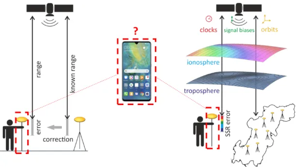
Figure 1.1: From left to right: range corrections for a user’s location transmitted by a refer- ence station and visualization of the SSR corrections generated by a network of reference sta- tions for a user’s position. One of the main questions addressed in the thesis is if the user can use a smartphone (center of the picture, within the dashed red-colored rectangle) instead of a geodetic-grade receiver (within the dashed red-colored rectangles) for RTK-level positioning.

Pictures provided by Geo++ GmbH.

clock, ionosphere, troposphere) can be estimated in real-time using GNSS observations from the network. Such a process is simplified in Fig. 1.1 (right side). Receiving the complete state information allows the user to generate GNSS corrections valid for their own position. If the corrections preserve the integer nature of the observations, AR becomes possible, enabling the so-called PPP-RTK positioning. In order to provide the corrections, the error states are repre- sented mathematically and consistently in the so-called State Space Representation (SSR).

One of the objectives of this dissertation is to develop techniques to support the improve- ment of high-accuracy satellite-based positioning solutions and the progress of the newest positioning applications. In the last years, an innovative GNSS-user application evolved: the use of GNSS raw data from Android devices for accurate and precise positioning. In 2016, the Android operation system enabled direct access to GNSS raw measurements in smartphones.

The new availability of data in the palm of the user’s hand, as depicted by Kenneth et al. (2015), triggered the intense and growing interest of many research groups to understand what can be achieved with such devices. The first question to answer is if the quality of the smartphone measurements is appropriate for positioning purposes. In particular, a reliable and continu- ous extraction of carrier phase measurements is essential to obtain RTK-level positioning and replace a user’s geodetic-grade receiver with a smartphone (as depicted in Fig. 1.1). Due to the cellphone’s main features (e.g. receiving a signal from any direction and especially dur- ing a phone-call), this objective has been recognized as challenging since the beginning of smartphone-based positioning research. A positive outcome to this question opens dynamic and fast innovations of new low-cost applications for satellite-based positioning.

Recently, the number of devices capable of providing GNSS measurements is growing and

growing. All the users equipped with cellphones with an Android version greater or equal to

7.0 are capable of retrieving GNSS raw-data. As reported by Liu (2020), in 2019, the number of

Android’s users was 1.6 billion worldwide. Also, worldwide, the most popular Android version

is Android 9 (Liu, 2020). This means that roughly 20% of the world population can access

provides a research opportunity to develop new techniques and applications. This can unveil applications making use of GNSS measurements.

Moreover, since 2018, smartphones have been equipped with dual-frequency and multi- constellation receivers. Nowadays, there are, to the best of the author’s knowledge, more than 40 smartphone models on the market that provide dual-frequency receivers. The dual- frequency capability enables the reduction of frequency-dependent errors that affect satellite measurements, e.g. the ionospheric delay. Taking advantage of such devices, promising results have been achieved already. A few decimeters accuracy positioning has been demonstrated with relatively short convergence time, i.e. a few minutes (e.g. Critchley-Marrows, 2020). How- ever, high-accuracy performance cannot be achieved in the user’s hand yet.

In this work, the main related issues are introduced and investigated, showing veri- fied methods to achieve reliable high-accuracy positioning using smartphones. The GNSS raw-measurements retrieved from the Android Application Programming Interface (API) are presented and analyzed. Statistical considerations are introduced, especially concerning the Carrier-to-Noise-ratio (C/N0) over long data-sets. In fact, smartphone measurements suffer from low C/N0 that has been demonstrated to be related not only to low-elevation satellites.

Also, site-dependent effects (e.g. multipath), which are a cause of error in GNSS-positioning, are investigated.

The most relevant issue related to doing positioning with smartphones is the antenna of the devices. In fact, most of the phones are equipped with an omnidirectional antenna that makes smartphones sensitive to surface reflections (i.e. multipath) of the nearby en- vironment. Along with multipath, the antenna pattern variations are the main source of station-dependent errors. Usually, to correct this electromagnetic effect, the geodetic antenna is calibrated, providing the so-called antenna corrections. Here, the calibration of a dual- frequency smartphone is reported together with the impact on positioning performance. The antenna calibration is demonstrated to be an essential step to achieve a reliable, accurate and highly precise estimated position. The positioning performance is investigated using SSR-based techniques assessing the potential of reliable RTK-level positioning.

In SSR-based positioning, atmospheric parameters computed by a network of GNSS ref- erence stations need to be interpolated for the user location. Atmospheric delays are GNSS error sources with a significant impact on the positioning performance and AR. As a conse- quence, the interpolation process has a direct impact on AR. Furthermore, in the last decades, the number of severe weather events has increased around the world. Focusing on Europe, Rädler et al. (2019) shows that the frequency of damaging convective weather events, including lightning, hail and severe wind gusts will likely increase over Europe until the end of this cen- tury. Moreover, during severe events like thunderstorms, the generated waves reach the up- per stages of the atmosphere, perturbing the ionosphere. These perturbations can lead to the so-called Traveling Ionosphere Disturbances (TIDs), which can significantly affect the GNSS measurements. Thunderstorms are only one of the possible sources of TIDs, which mainly de- pend on solar activity. The increasing number of severe events raises interest in investigating the impact of such events on the positioning performance. In this dissertation, the interpo- lation quality is analyzed along with the benefit of using external information retrieved from atmospheric models. Accordingly, multiple interpolation techniques are investigated and new methods are proposed to make the AR process more robust during severe weather and TID events. These alternative methods take advantage of external atmospheric models that have been becoming more and more accurate during the last years.

The primary objective of this thesis is to investigate and show the potential for RTK-level

smartphone-based positioning using state space GNSS augmentation techniques. Besides,

one of the main issues in SSR-based positioning is assessed, investigating the interpolation

process of atmospheric parameters. The following section introduces the structure of the the-

sis.

Outline

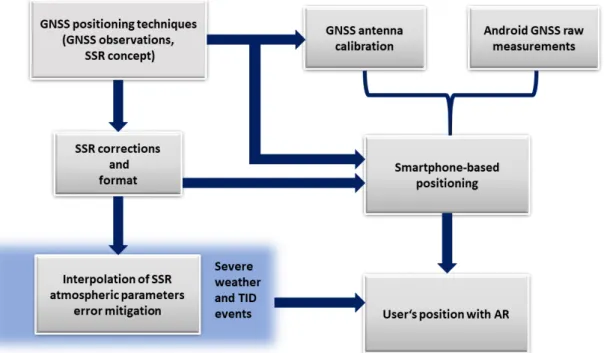
Fig. 1.2 shows a schematic representation of the connection between the topics of Chapters 2- 4. The central scientific questions are:

• which level of accuracy and precision can be achieved in smartphone-based position- ing? Can a user replace a geodetic-grade rover receiver with a smartphone (as depicted in Fig. 1.1) ?

• What is the impact of interpolation errors of SSR atmospheric corrections on position- ing for a user within a network of GNSS reference stations? Can this error be mitigated during severe weather and TID events by including external atmospheric model infor- mation?

In order to address these questions, multiple aspects are investigated through the thesis. Apart from the introductory chapter Chapter 2, each chapter has a motivation and discussion sec- tions. While the motivation section presents the reasons behind the analysis, the discussion section summarizes the primary outcome and examines the possible benefits of the investiga- tion.

The positioning techniques employed in this work are introduced in Chapter 2 along with the description of the GNSS observations. In particular, the central SSR concept is presented.

Chapter 2 introduces the main concepts and notation used through the thesis. In addition, the use of SSR corrections and the format utilized for their transmission are presented.

A method to reconstruct GNSS observations from the raw measurements retrieved from the Android API and to assure their use for positioning purposes is reported in Chapter 3. Also, the quality of GNSS raw measurements for positioning applications is investigated. In sum- mary, Chapter 3 reports the potential of cm-level positioning using smartphones’ measure- ments by employing the positioning techniques introduced in Chapter 2.

Figure 1.2: Schematic representation of the connection between the topics of Chapters 2-4,

having the final objective to compute the user’s position with AR.

servations and SSR concepts presented in Chapter 2. In this work, the GNSS smartphone’s an- tenna is calibrated by an absolute robot-based field calibration. The results of the calibration and the impact of using it in the positioning algorithm are reported achieving an estimated user’s position with successful AR.

In Chapter 5, the interpolation error of SSR atmospheric parameters is investigated. Multi- ple interpolation techniques, e.g Inverse Distance Weighted (IDW), Ordinary Kriging (OK) and Weighted Least Squares (WLS), are analyzed. In addition, alternative approaches are proposed to mitigate the interpolation error during specific severe weather and TID events. As examples, two severe weather events in northern Europe in 2017, and one TID event over Japan in 2019 have been analyzed. The final aim of the interpolation analysis is to provide guidelines to have a robust AR for high-accuracy and precision positioning for a user’s location within a network.

Also, the impact of an SSR ionospheric mismodeling on the estimated position is assessed in terms of AR and positioning error.

Finally, in Chapter 6, the main conclusions are summarized with an outlook for further

research steps.

2. GNSS Positioning Techniques

2.1 The GNSS observation equations

The main idea behind GNSS-based positioning is to localize a point on the Earth’s surface by making use of the observed range between the point and the GNSS satellite. The observed range is related to a signal broadcast by GNSS satellites traveling towards the Earth’s surface until being received by an appropriate device (i.e. a receiver). The navigation satellites typi- cally make use of the L-band frequency, i.e. the band between 1 and 2 GHz, to broadcast their signals (e.g. Teunissen and Montenbruck, 2017). Taking into account the traveling time of the signal and its velocity, the range can be reconstructed as follows:

ρ = c(t

− t

), (2.1)

where c is the speed of light, t

the acquisition time and t

the emission time of the signal. The localization of a point on the Earth’s surface is expressed in coordinates in a specific reference frame. Therefore, the coordinates of the receiver can be written in the following way:

x

= x

+ ρ u ˆ

, (2.2)

where x

is the receiver vector with components the coordinates of the receiver, x

is the satel- lite vector and ˆ u

is the unit vector of the radial direction from the satellite towards the re- ceiver position. The components of both x

and x

are expressed w.r.t. the same reference system, e.g. the Earth-Centered Earth-Fixed (ECEF), the International Terrestrial Reference Frame (ITRF), and the World Geodetic System 1984 (WGS84) systems.

In this dissertation, a user will be considered as someone who utilizes a GNSS receiver to gather measurements of the GNSS signals to localize a position, i.e. to express the receiver coordinates w.r.t. a defined reference system. The computation of the position vector of the receiver x

goes through an estimation process using GNSS observations as described by many authors (e.g. Teunissen and Montenbruck, 2017). Conceptually, the GNSS observation is the range ρ. In general, the estimation process can be summarized by the following equation model:

f (x) = y + ν , (2.3)

where x is the vector of the parameters that need to be estimated (including x

), y is the ob- servation vector, ν is the residual vector and f is a non-linear functional relationship between observations and parameters. It is worth mentioning that all the vectors of Eq. 2.3 are func- tions of the time. The principles of the estimation of the parameters using GNSS observations will be introduced in Section 2.2.

In their measurements, the user observes the range ρ expressed in Eq. 2.1. However, in Eq. 2.1, many physical aspects related to a broadcast and received radio-frequency signal trav- eling in space and atmosphere have been neglected. First of all, synchronization delays of the satellite’s and receiver’s clocks need to be taken into account. Secondly, the signal travels through the atmosphere, which is not the vacuum but a medium. Hence, the signal is delayed.

In their path to the receiver, the signal can be deviated by impinging other surfaces and causing

a range distortion. Another aspect is the electromagnetism of the antennas used to broadcast

and acquire the signal, which introduces delays that cannot be neglected. Furthermore, the

measurements are affected by the relative motion between user and satellite (e.g. the Earth’s

rotation) and by the relativistic effects. Finally, the hardware used to transmit and receive the

2.1. The GNSS observation equations signal introduces delays. Therefore, the expression of the observation that is observed by the user cannot be defined by the range expressed by Eq. 2.1, and it needs to be modified to take into account all the error sources. The observation is the so-called pseudorange, and it will be described in the following section.

Many textbooks present the equations of the GNSS observations (e.g. Teunissen and Mon- tenbruck, 2017)), and it is not the main purpose of this dissertation to provide a fully detailed description of all the related aspects. However, it is worth introducing the notation that is used in the whole work. For further details about the basic concepts of GNSS measurements, the reader is referred to Spilker Jr et al. (1996); Parkinson et al. (1996); Montenbruck and Gill (2002);

Seeber (2003); Misra and Enge (2006); Teunissen and Montenbruck (2017).

2.1.1 Pseudorange measurements

The GNSS receiver generates a replica of the received signal as best as possible by using satel- lites known pseudo-random-code and its internal frequency source. The alignment of the re- ceiver code to the received signal is done by the receiver’s Delay Lock Loop (DLL). The nec- essary time shift combined with the code-related information provided by the satellite navi- gation data determines the apparent travel time of the signal. Multiplying the apparent travel time with the speed of light (in the same way done in Eq. 2.1), the apparent range, i.e. the pseu- dorange, is obtained. As aforementioned, this quantity differs from the actual range because of the misalignment between the receiver’s and satellite’s clocks. Furthermore, the signal re- ception is affected by other error sources, like e.g. atmospheric refraction. Taking into account all the introduced considerations, at a specific epoch t a receiver r observes the signal j of the satellite s as follows:

p

(t

) =ρ

(t

) + c ³

d t

(t

) − d t

(t

) + δ t

(t

, t

) ´ + c ³

d

− d

´ + I

(t

) + T

(t

) + ξ

(t

, t

) + µ

(t

) + e

(t

).

(2.4)

In Eq. 2.4, t

and t

are the signal acquisition and emission time, respectively, and ρ

(t

) is the geometric range (i.e. Eq. 2.1 in an ideal scenario without any delays and errors). The delays and error sources that appear in the equation can be summarized as follows:

• d t

(t

) − d t

(t

) + δ t

(t

, t

) is the delay due to the receiver’s (d t

(t

)) and satellite’s (d t

(t

)) clock offsets, and the relativistic effects ( δ t

(t

, t

)). More information about the relativistic effects can be found in, e.g., Ashby (2003) and Teunissen and Montenbruck (2017).

• d

− d

is the delay caused by the hardware.

• I

(t

) + T

(t

) is the range deviation due to the signal refraction in ionosphere (I

) and troposphere (T

(t

)).

• ξ

(t

, t

)+µ

(t

) is the station dependent error, made of two contributions: the Group Delay Variations (GDV) ξ

(t

, t

) due to the receiver’s and satellite’s antennas and the multipath (MP) effect µ

(t

).

• e

(t

) is the receiver’s code noise.

2.1.2 Carrier phase measurements

Along with the pseudorange, the receiver also measures the signal’s carrier phase from its Phase Lock Loop (PLL). The measurement is a fractional phase shift of the receiver’s replica and of the received carrier phase. The carrier phase measurements are more precise (i.e. few mm) than the pseudorange measurements (i.e. dm-level) because of the short wavelength of roughly 20 cm (compared to the 293 m of the GPS C/A code). However, satellite navigation data cannot be used to obtain unambiguous carrier phase observations. The reason is that the integer number of cycles of the phase between the transmitter and receiver when the track- ing starts is unknown, causing the ambiguous nature of the phase observations. Similar to the pseudorange, the carrier phase observation equation can be expressed in the following way:

φ

(t

) =ρ

(t

) + c ³

d t

(t

) − d t

(t

) +δ t

(t

, t

) ´ + c ³

d

− d

´

− I

(t

) + T

(t

) + λ

³ ω

(t

, t

) + N

´ + ζ

(t

, t

) + µ

(t

) + ²

(t

),

(2.5)

where ζ

(t

, t

) is the Phase Center Variations (PCV) component due to the receiver’s and satellite’s antennas. The wind-up correction, ω

(t

, t

), accounts for a change in the measured phase due to a change in the relative geometry between satellite and receiver antenna (e.g.

Hauschild, 2017; Wu et al., 1993). Here, ²

(t

) is a residual phase noise.

The comparison between Eq. 2.4 and Eq. 2.5 highlights the difference in sign of the iono- spheric impact. The sign change is a consequence of the frequency-dependency of the signal propagation through a dispersive medium and different velocity of carrier and the modulation of the signal (e.g. Langley, 1998a; Petrie, 2011; Teunissen and Montenbruck, 2017).

2.1.3 Atmospheric delays

The GNSS signal interactions with ionosphere and troposphere are two of the major GNSS error sources. In terms of range, the tropospheric delay can be up to ~2.3-2.6 m at the zenith and ~25 m for elevations close to five degrees (at sea level, the values depend on the location).

Concerning the ionosphere, the errors can vary between ~1 m and tens of meters at the zenith multiplied by roughly a factor of three at low elevation angles when using a single layer model of the ionosphere (Schaer, 1999). Atmospheric delays are obtained by integrating the refractive index n along the signal path. The refractive index depends on permittivity and permeability of the medium that the signal is passing through, which vary in space and time. Since the value of n is close to one, many publications introduce the so-called refractivity N as follows:

N = (n − 1) × 10

. (2.6)

Although both delays are related to the signal propagation through a medium, the physical processes behind ionospheric and tropospheric delays are different. On the one hand, the ionospheric delay is mainly related to the Sun’s activity and the interaction between ionized particles. On the other hand, the tropospheric delay is related to the local weather conditions.

In fact, the troposphere is the lowest layer of the atmosphere, i.e. altitude < 16 km (at the

equator), while the ionosphere approximately covers the altitude between 80 km and 1000

km.

2.1. The GNSS observation equations A significant difference between the two atmospheric layers is that while the ionosphere is a dispersive medium, the troposphere is not. The troposphere can be seen as a layer made of gas where small distances (roughly 0.1 nm) and strong forces with fast oscillations among particles are involved. The ionosphere, instead, is made of plasma whose particles are char- acterized by large distances (roughly 0.1 mm), weak forces and slow oscillations. The plasma frequency, i.e. the frequency at which electrons oscillate about their equilibrium positions, is up to 22 MHz for the F2-peak (350 km in a Chapman layer description, see, e.g., Petrie (2011) for a complete review), where the electron density is N

= 6 × 10

electrons m

. Hence, the maximum plasma frequency is 100 times lower than the L-band GNSS frequencies (e.g. L1 fre- quency is 1.575 GHz). In the troposphere, instead, the main transition effects are related to the atomic frequency that is about some hundreds of THz, i.e. five orders greater than the L1 GNSS frequency. Therefore, GNSS frequencies are far below atomic resonances, but far above elec- tron (plasma) resonances that makes the ionosphere a dispersive medium. This fact causes the frequency dependency of the ionospheric delay I

compared to the tropospheric delay T

. The dispersive nature implies the different phase (carrier) and group (code) velocity re- sulting in the opposite sign in Eq. 2.4 and Eq. 2.5.

The tropospheric delay

Details about the modeling of the troposphere can be found in multiple textbooks (e.g. Te- unissen and Montenbruck, 2017) or dissertations (e.g. Kleijer, 2004). Here, the purpose is to provide the reader useful information to analyse the results of this dissertation properly. The slant tropospheric delay, T

, depends on:

• dry gases, varying little over temporal and spatial scales of hours and km;

• water vapor, with highly variable spatial and temporal distributions.

For a satellite s and receiver r , the slant tropospheric delay is computed by the following inte- gral (e.g. Hauschild, 2017):

T

= 10

Z

s

N d l, (2.7)

where N is the tropospheric refractivity, and l is the propagation path of the signal. As the troposphere can be consider as moist air, the refractivity N can be expressed as the sum of a dry (hydrostatic) N

(depending only on pressure and temperature) and wet component N

, depending on water vapor pressure (Essen and Froome, 1951):

N = k

p T + k

e

T + k

e T

,

= N

+ N

,

(2.8) where T is the temperature, p and e are the total pressure and partial pressure of the wet con- stituent, respectively. Furthermore, the constant k

is computed as follows (e.g. Hauschild, 2017):

k

= k

− k

R

R

, (2.9)

where R

and R

denote the gas constants for dry air and water vapor, respectively. The three constants are given as k1 = 77.6 K/mbar, k2 = 64.8 K/mbar and k3 = 3.776 × 10

K

/mbar (Thayer, 1974). During the years, multiple models have been developed. The models relate the state of the atmosphere at an arbitrary height to the atmospheric parameters at the user height and thus allow the integration of Eq. 2.7 into zenith direction (Hauschild, 2017). As a consequence, Eq. 2.7 can be re-written in the following way:

T

= m

( ε )Z H D

+ m

( ε )Z W D

+ m

( ε )[G

cos ( α ) + G

sin ( α )]. (2.10)

In Eq. 2.10, m

( ε ) and m

( ε ) are the so-called mapping functions, which map the Zenith Hydrostatic Delay (ZHD) and Zenith Wet Delay (ZWD) into the direction of the line of sight through the elevation ². The elevation-dependent mapping function m

(²) relates the North and East components of the tropospheric horizontal gradient G = [G

,G

]. G describes an azimuthal asymmetry of the delay through the dependency on the azimuth α . Horizontal gra- dients are needed to consider a systematic component in the North/South direction towards the equator due to the atmospheric bulge (MacMillan and Ma, 1997). Typical values of the magnitude of the gradients are roughly 0.5 mm but can reach or exceed 1 mm (MacMillan and Ma, 1997; Petit and Luzum, 2010), as shown in Chapter 5.

The sum of zenith dry (hydrostatic) and wet components gives the Zenith Tropospheric Delay (ZTD). Accordingly, Eq. 2.10 can be written as:

T

= m

( ε )Z T D

+ m

( ε )[G

cos ( α ) + G

sin ( α )], (2.11) where m

(ε) is the function that maps the Z T D into the line of sight direction. While the hydrostatic delay component can be accurately computed based on the Saastamoinen model (Saastamoinen, 1972; Petit and Luzum, 2010), the wet component needs to be estimated by the GNSS positioning algorithm.

Several mapping functions have been developed by many authors, e.g. Marini (Marini, 1972), Herring (Herring, 1992), Niell (Niell, 1996), Vienna Mapping Functions (VMF) (Böhm et al., 2006b), and Global Mapping Functions (GMF) (Böhm et al., 2006a). More details about the basic description of hydrostatic and wet delays, and mapping functions can be found in, e.g., Seeber (2003); Petit and Luzum (2010); Hauschild (2017); Hobiger and Jakowski (2017).

In the last years, many studies have been carried out to develop Numerical Weather Mod- els (NWM), like, e.g., the European Center for Medium-Range Weather Forecasts (ECMWF) and the Global Forecasting System (GFS). Based on the physical quantities provided by NWM, a user can retrieve tropospheric delays. Examples of the methodology to generate slant and zenith tropospheric delays can be found in, e.g., Nafisi et al. (2011); Zus et al. (2012). In Chap- ter 5, the benefit of using external information like NWM for GNSS-based positioning is inves- tigated.

The ionospheric delay

The propagation of an electromagnetic wave through the ionosphere has been investigated deeply. For L-band signal specific assumptions can be made:

• the effects of electron collisions are neglected;

• the plasma is a cold plasma (i.e. the velocities of the electrons’ thermal motions are much less than the phase velocity of the wave):

• there is a uniform magnetic field.

See e.g. Yeh et al. (1972); Davies (1990); Petrie (2011) for further information. These assump- tions allow to describe the refractivity index as a function of the electron density N

in the generally known as Appleton-Lassen equation (Lassen, 1927; Appleton, 1932). The Appleton- Lassen equation has been studied and re-arranged by multiple authors and a review can be found in, e.g., Petrie (2011). It is out of the scope of this work to go into the details of the elec- tromagnetic equations. The main focus is on the effects on the pseudorange and carrier phase observations. Integrating the effect of the refractive index along the curve path and neglect- ing the second and third-order refractive index effects (e.g. Petrie, 2011), the ionospheric delay yields:

I

= 40.3 × 10

f

Z

s

N

d l, (2.12)