Solving the Fisher/KPP Evolution on the Globe

SOLVING THE FISHER/KPP EVOLUTION ON THE GLOBE

Written by

AMÉLIE JUSTINE LOHER Supervised by

PROF. DR. RALF HIPTMAIR

BACHELOR THESIS

EIDGENÖSSISCHE TECHNISCHE HOCHSCHULE ETH ZURICH Department of Mathematics

MAY 2020

ABSTRACT

The Fisher equation was originally intended to model the propagation of advantageous genes.

We use this reaction-diffusion equation equipped with non-local boundary conditions to model the propagation of individuals across geographical maps. These boundary condition account for a non-local "diffusion" across channels. The results represent the dispersal of the Homo Sapiens across the globe. The discretisation is based on finite element methods.

Moreover, the Strang splitting method is employed to cope with the diffusion and reaction term separately.

TABLE OF CONTENTS

Page

ABSTRACT . . . ii

1 Introduction . . . 1

1.1 Origins of the Fisher-KPP Equation . . . 1

1.2 Earlier works on Population Dynamics . . . 3

2 Mathematical Derivation . . . 4

2.1 Problem Formulation . . . 4

2.2 Variational Formulation . . . 5

3 Discretisation: Method of Lines . . . 7

3.1 Galerkin Discretisation . . . 7

3.2 Strang Splitting Method . . . 9

3.2.1 Diffusion Term . . . 10

3.2.2 Reaction Term . . . 12

4 Implementation. . . 14

4.1 Mesh Generation . . . 14

4.1.1 Raw data . . . 14

4.1.2 QGIS . . . 15

4.1.3 Gmsh . . . 15

4.2 LehrFEM++ . . . 16

4.2.1 Input-Output Reader . . . 16

4.2.2 Galerkin Matrices . . . 16

4.2.3 Visualisation . . . 18

5 Model Problem . . . 19

5.1 Travelling Wave Solutions . . . 19

5.2 Convergence Analysis . . . 27

5.2.1 Convergence Studies for Mesh Width . . . 30

5.2.2 Convergence Studies for Time Step Sizes . . . 32

5.2.3 Convergence Studies for Mesh Width linked to Time Step Sizes . . 32

6 Results . . . 36

6.1 Parameters . . . 37

6.1.1 First Approach . . . 37

6.1.2 Second Approach . . . 38

6.2 Visualisation . . . 38

7 Conclusions . . . 40 APPENDIX

ACKNOWLEDGEMENT

The author expresses her distinct gratifications to Prof. Dr. Hiptmair for the initiation of this thesis and for his continuous guidance. Throughout the development of this project Prof. Dr. Hiptmair has provided helpful advice, supportive suggestions and encouraging thoughts.

Chapter One Introduction

1.1 Origins of the Fisher-KPP Equation

In 1937, two articles were published concerning the spatial propagation of advantageous genes in a population. The author of the first article was Fisher [4], who studied the propagation of dominant genes in one spatial dimension. He modelled the proportion of the population located at pointx at time t possessing the dominant gene withu(t, x), and thus there holds 0≤u≤1. To take into account natural selection, he used Verhulst’s logistics equation

∂u

∂t =λu(1−u), (1.1)

for λ ∈R>0. Moreover, Fisher modelled the diffusion of the offspring of an individual with a favourable gene in a neighbourhood of xby adding a diffusion term,

∂u

∂t =λu(1−u) +c∂²u

∂x². (1.2)

Fisher then showed the existence of infinitely many travelling wave solutions for (1.2), that is solutions of the form u(t, x) =u(x−vt) satisfying

0≤u(t, x)≤1, lim

x→−∞u(t, x) = 0, lim

x→∞u(t, x) = 1, (1.3)

provided thatv ≥2√

λc. Thus, travelling waves of constant speedv along thex-axis connect the steady stateu= 1 of the advantageous gene with the stateu= 0 lacking any such gene.

The second article was published by Kolmogorov, Petrovsky and Piskunov [8]. Simi- larly, it concerned the propagation of dominant genes. Based on Mendelian genetics, they considered

∂u

∂t =f(u) +c∂²u

∂x², (1.4)

where u represents again the density of favourable genes, and wheref(u)satisfies

f(0) = 0 =f(1), f⁰(0) >0, (1.5)

and for 0< u <1,

f(u)>0, f⁰(u)< f⁰(0). (1.6)

Assuming that the initial condition satisfies

0≤u(0, x)≤1, (1.7)

as well as

u(0, x) = 0 ∀x < x₁,

u(0, x) = 1 ∀x > x₂ ≥x₁, (1.8)

the authors proved that the gene propagates at constant speed v = 2p

f⁰(0)c. Furthermore, under these assumptions on the initial condition, (1.4) admits a unique solution which fulfils 0 < u(t, x) < 1 for all (t, x) ∈ R×R^≥0, and which converges towards a wave profile prop- agating at finite speed v. Thereof, we may conclude that the initial gradient governs the speed of propagation. It has been shown that for compactly supported initial datum, wave fronts evolve to solutions of minimal speed of propagation [10].

Let me emphasise that in case of the Fisher’s equation (1.2), we have

f(u) =λu(1−u). (1.9)

Notice that this implies

f⁰(u) = λ(1−2u). (1.10)

Therefore we realise that for λ∈R>0,

f(0) = 0 =f(1), f⁰(0) =λ >0, (1.11) and for 0< u <1,

f(u)>0, f⁰(u) = λ(1−2u)< λ=f⁰(0). (1.12) Hence Fisher’s equation satisfies the conditions (1.5), (1.6). If we now further suppose that (1.7) and (1.8) are fulfilled, there holds according to Kolmogorov, Petrovsky and Piskunov [8] that there is a unique solution propagating at constant speed

v = 2p

f⁰(0)c= 2√

λc. (1.13)

Consequently, the solutions propagate at finite speed.

On the other hand, we realise that in the case λ = 0, Fisher’s equation (1.2) coincides with the heat equation, admitting infinite speed of propagation [1]. However, note that in this case the assumption (1.5) is violated.

In conclusion, in our case with constant or piecewise constant values for the diffusion coefficient c, we anticipate solutions with finite speed of propagation. The succeeding nu- merical experiments meet this expectation. In all simulations performed below aiming at the exhibition of travelling wave solutions originating from compactly supported initial datum on bounded domains, we observe numerically a finite speed of propagation, see section 5.1.

In two and three spatial dimensions, propagating wave fronts may evolve to some station- ary states. Albeit these need not be unique, they usually possess some kind of symmetry.

Under the assumption that a stationary wave propagates along the x-axis, travelling wave solutions read in the two-dimensional case for some x= (x₁, x₂)∈R²,

u(t,x) = u(x₁−V t, x₂), (1.14)

whereV is the velocity of the wave. In the two-dimensional case with two stationary states, we may expect a reflection symmetry for the wave front with respect to its propagation direction [2].

1.2 Earlier works on Population Dynamics

In 2017, W. P. Petersen et al. published a paper [14] on the numerical simulation of Fisher’s equation on geographical maps based on a finite difference scheme, employing a Godunov- type splitting. Following their main goal to model population dynamics, we discuss in the sequel another approach based on finite element methods, where we employ the Strang splitting method.

Our interests are drawn to study the evolution of our population density over space and time. Since we want to model the dispersal of the Homo Sapiens on the globe, our time horizon starts200000years ago, and ranges up to 15000years ago. Moreover, our domainΩ represents the earth’s surface. We model the humans’ evolution with the Fisher’s equation, a special case of the Kolmogorov-Petrovsky-Piscounov equation.

Chapter Two

Mathematical Derivation

2.1 Problem Formulation

LetΩ⊂R² be a bounded domain, let T ∈R^≥0 be the final time. We consider a continuous function u: [0, T]×Ω→R, representing the population density.

Assuming that u(t)∈C²(Ω), we have

∂u

∂t =div(c(t,x)grad u) +λ (1− u

K(t,x))u in[0, T]×Ω (2.1) where c : [0, T] ×Ω → R denotes the diffusion coefficient, λ ∈ R>0 is a constant growth factor, and K : [0, T]×Ω→R describes the carrying capacity.

Note that our domainΩneed not be connected. Indeed accounting for the various islands over the globe, it is certain not to be. Thus it is of great importance to impose boundary conditions describing properly the dispersal over straits, whenever two land territories are close enough such that humans crossed the sea. Therefore we establish non-local boundary conditions.

Let us consider a point on the boundary of Ω, x ∈ ∂Ω. Let L ∈ N denote the number of connected components of our domain Ω. The boundary of Ω consists of all the curves enclosing a single connected component. Thus we may number these curvesΓ_i fori∈1, ..., L such that

L

S

i=1

Γ_i =∂Ω, whereΓ_i∩Γ_j =∅ fori6=j. For any suchx, we then have thatx∈Γ_i for some i∈1, ..., L.

To account for the dispersal over the sea, we proceed as follows: let j : [0, T]×Ω → Ω model the flow of individuals in our domain. By Fourier’s Law, we find that

j(t,x) =−c(t,x) grad u in Ω. (2.2) At the boundary, we impose the non-local flux condition

j(t,x)·n(x) = Z

∂Ω

g(x,y) (u(t,x)−u(t,y))dS(y), (2.3)

where n ∈ R² denotes the outer normal vector, and where g : ∂Ω×∂Ω → R is a kernel function decaying with increasing distance between x and y. The intuition behind (2.3) is that with a larger distance between two coastlines the difficulty of crossing the sea increases, and thus the probability of the actual happening of such traversal diminishes. Moreover, the gain of population on the point of arrival at ∂Ωevidently implies the loss of population on Γ_i. Note that by taking all of the boundary ∂Ω into consideration as possible arrival sites, we include the possibility of travelling along the coastline of departure Γ_i. Combining equation (2.2) with (2.3), we obtain

−c(t,x) grad u·n(x) = Z

∂Ω

g(x,y) (u(t,x)−u(t,y))dS(y). (2.4) Equation (2.4) connote the non-local boundary condition for our model.

Finally, starting with an initial population denoted by u0 : Ω → R, we obtain the following model:















∂u

∂t =div( c(t,x) grad u) +λ (1− u

K(t,x)) u in Ω

−c(t,x) grad u·n(x) = Z

∂Ω

g(x,y) (u(t,x)−u(t,y))dS(y) on ∂Ω u(0,x) = u₀(x) in Ω

(2.5)

2.2 Variational Formulation

In the sequel we derive the weak formulation for (2.5). Letv ∈C_c^∞(Ω)be a testing function.

Integrating (2.1) over Ω yields Z

Ω

∂u

∂t(t,x) v(x)dx= Z

Ω

div( c(t,x) grad u(t,x)v(x) dx +

Z

Ω

λ (1− u(t,x)

K(t,x)) u(t,x)v(x) dx

=− Z

Ω

c(t,x) grad u(t,x)·grad v(x)dx +

Z

∂Ω

c(t,x) grad u(t,x)·n(x) v(x) dS(x) + Z

Ω

λ (1− u(t,x)

K(t,x)) u(t,x)v(x) dx

=− Z

Ω

c(t,x) grad u(t,x)·grad v(x)dx

− Z

∂Ω

Z

∂Ω

g(x,y) (u(t,x)−u(t,y))v(x)dS(y)dS(x) +

Z

Ω

λ (1− u(t,x)

K(t,x)) u(t,x)v(x) dx

where we have used Green’s first formula [7] and the non-local boundary conditions of equa- tion (2.5). Choosing suitable function spaces leads us to the following variational formulation:

We seek [0, T]3t →u(t)∈H¹(Ω) satisfying Z

Ω

∂u

∂t(t,x) v(x) dx+ Z

Ω

c(t,x) grad u(t,x)·grad v(x) dx +

Z

∂Ω

Z

∂Ω

g(x,y) (u(t,x)−u(t,y))v(x) dS(y)dS(x)

− Z

Ω

λ (1− u(t,x)

K(t,x)) u(t,x)v(x) dx= 0, ∀v ∈H¹(Ω)

(2.6)

with u(0,x) = u₀(x) for x∈Ω.

Let u, v ∈ H¹(Ω). Let us introduce bilinear functionals m, a, b : H¹(Ω)×H¹(Ω) → R with

m(∂u

∂t(t), v) :=

Z

Ω

∂u

∂t(t,x) v(x) dx= ∂

∂t Z

Ω

u(t,x)v(x) dx= ∂

∂tm(u(t), v), (2.7) a(u(t), v) :=

Z

Ω

c(t,x)grad u(t,x)·grad v(x)dx, (2.8)

b(u(t), v) :=

Z

∂Ω

Z

∂Ω

g(x,y) (u(t,x)−u(t,y)) v(x) dS(y)dS(x), (2.9) and finally for the non-linear term, we write r : H¹(Ω)×H¹(Ω) → R, a mapping linear in its second argument, defined as

r(u(t);v) :=

Z

Ω

λ (1− u(t,x)

K(t,x)) u(t,x)v(x) dx. (2.10) With these notations, we arrive at the following formulation equivalent to equation (2.6):

we seek[0, T]3t→u(t)∈H¹(Ω) satisfying







∂

∂tm(u(t), v) +a(u(t), v) +b(u(t), v)−r(u(t);v) = 0, ∀v ∈H¹(Ω) u(0) =u₀ ∈H¹(Ω)

(2.11)

Chapter Three

Discretisation: Method of Lines

3.1 Galerkin Discretisation

We pursue a method of lines approach [7], that is we first proceed with a spatial semi- discretisation for equation (2.11).

The spatial Galerkin semi-discretisation relies on linear Lagrangian finite elements on a triangular mesh M of Ω with the lowest-order Lagrangian finite element space S₁⁰(M) using a polygonal approximation of the boundary. In a first step, we replace our infinite- dimensional Hilbert space H¹(Ω) =: V0 with a finite dimensional subspace V0,h ⊂V0. Thus, we seek[0, T]3t→uh(t)∈V0,h satisfying







∂

∂tm(u_h(t), v) +a(u_h(t), v) +b(u_h(t), v)−r(u_h(t);v) = 0, ∀v ∈V_0,h u_h(0) =u_0,h ∈V_0,h

(3.1) where u_0,h ∈V_0,h represents the projection of u₀ ∈V₀ onto V_0,h =S₁⁰(M).

As a second step, we choose an ordered basis B_h = {b¹_h, ..., b^N_h}, where N := dim(V_0,h), such thatV_0,h =span{B_h}. Then we may expandu_h, v_h ∈V_0,hin terms of this basis functions as u_h(t) =PN

i=1µ_i(t)bⁱ_h and v_h =PN

j=1ν_jb^j_h, whereµ_i, ν_j ∈ R fori, j ∈ {1, ..., N}. Inserting the corresponding expansions into equation (3.1) gives

∂

∂tm(

N

X

i=1

µ_i(t)bⁱ_h,

N

X

j=1

ν_jb^j_h) +a(

N

X

i=1

µ_i(t)bⁱ_h,

N

X

j=1

ν_jb^j_h) +b(

N

X

i=1

µ_i(t)bⁱ_h,

N

X

j=1

ν_jb^j_h)

−r(

N

X

i=1

µ_i(t)bⁱ_h;

N

X

j=1

ν_jb^j_h) = 0, ∀ν_j ∈R, j ∈ {1, ..., N}.

Equivalently,

N

X

i=1 N

X

j=1

ν_j ( ∂

∂tm(µ_i(t)bⁱ_h, b^j_h) +a(µ_i(t)bⁱ_h, b^j_h) +b(µ_i(t)bⁱ_h, b^j_h)−r(

N

X

l=1

µ_l(t)b^l_h;b^j_h) ) = 0,

∀ν_j ∈R, j ∈ {1, ..., N}.

Using Lemma 2.2.2.3 in [7], we find

N

X

i=1

( ∂µi

∂t (t)m(bⁱ_h, b^j_h) +µi(t)a(bⁱ_h, b^j_h) +µi(t)b(bⁱ_h, b^j_h)−r(

N

X

l=1

µl(t)b^l_h;b^j_h) ) = 0, j ∈ {1, ..., N}.

Thus we seek [0, T]3t→µi(t)∈R, i∈ {1, ..., N}satisfying























N

X

i=1

( ∂µ_i

∂t (t)m(bⁱ_h, b^j_h) +µ_i(t)a(bⁱ_h, b^j_h) +µ_i(t)b(bⁱ_h, b^j_h)−r(

N

X

l=1

µ_l(t)b^l_h;b^j_h) ) = 0, j ∈ {1, ..., N}

N

X

i=1

µi(0)bⁱ_h =u0,h ∈V0,h

Let us now introduce suitable Galerkin matrices M, A, B ∈R^N,N, where

M:= [m(bⁱ_h, b^j_h)]^N_i,j=1 (3.2) A:= [a(bⁱ_h, b^j_h)]^N_i,j=1 (3.3) B := [b(bⁱ_h, b^j_h)]^N_i,j=1 (3.4) These matrices will be assembled from the entries of the local element matrices on the reference triangle, see section 4.2.2 below. Let µ := (µ₁, µ₂, ..., µ_N)^T ∈ R^N. For the non- linear term write ρ: [0, T]×R^N →R^N with

ρ(t,µ(t)) = [r(

N

X

l=1

µl(t)b^l_h;b^j_h)]^N_j=1. (3.5) We then seek [0, T]3t→µ(t)∈R^N satisfying







M{∂µ

∂t(t)}+Aµ(t) +Bµ(t)−ρ(t,µ(t)) = 0 µ(0) =µ₀

(3.6) where µ₀ is the coefficient vector for the projection of u₀ onto V_0,h. We can recover the discrete solution with u_h =PN

i=1µ_i(t)bⁱ_h.

Let me remark that by means of suitable numerical quadrature it is often possible to obtain diagonal mass matrices, a trick called mass lumping [7]. In our case, we will make use of mass lumping (see Remark 6.3.4.18 in [7]) based on the composite trapezoidal rule, (2.3.3.8) in [7]. This allows the efficient computation of the inverse of the mass matrix Min (3.6).

We have thus obtained a semi-discrete evolution problem for the coefficient vector µ ∈ R^N. We acquire the full discretisation for equation (3.6) by employing a suitable time stepping method.

3.2 Strang Splitting Method

We apply the Strang splitting method [6] to solve the ordinary differential equation (3.6).

To this end, first note that since the bilinear form m in (2.7) is symmetric and positive definite, we have that M is invertible [7]. Hence we may rewrite (3.6) as







∂µ

∂t(t) =f(t,µ) +g(t,µ) µ(0) =µ₀

(3.7)

wheref(t,µ) :=−M⁻¹(A+B)µ(t), andg(t,µ) :=M⁻¹ρ(t,µ(t)). Splitting equation (3.7) into two parts, ^∂µ_∂t(t) =f(t,µ) and ^∂µ_∂t(t) = g(t,µ), allows to solve each part separately.

Consider the following mappings for fixed t ∈[0, T]:

Φ^t_f : (

R^N →R^N

µ₀ →µ(t) (3.8)

and

Φ^t_g : (

R^N →R^N

µ₀ →µ(t) (3.9)

corresponding to ^∂µ_∂t(t) = f(t,µ) and ^∂µ_∂t(t) = g(t,µ), respectively, with appropriate initial condition µ(0) = µ₀. These are well-defined mappings of the state space into itself, see [6].

We can now define evolution operators for each part:

Φ_f :

( [0, T]×R^N →R^N

(t,µ₀)→Φ^t_f(µ₀) :=µ(t) (3.10) Φg :

( [0, T]×R^N →R^N

(t,µ₀)→Φ^t_g(µ₀) :=µ(t) (3.11) Then we find that ^∂Φ_∂t^f(t,µ) = f(t,Φ^t_f(µ)), as well as ^∂Φ_∂t^g(t,µ) = g(t,Φ^t_g(µ)).

We proceed by introducing an equidistant temporal mesh with nodes 0 = t₀ < t₁ < ... <

t_M−1 < t_M = T, M ∈ N. Let τ := t₁ −t₀ be the step size. This allows to discretise the mappings (3.8), (3.9), as well as the evolution operators (3.10) and (3.11). In particular we define the discrete mapping

Ψ^τ :=Φ^{τ /2}_f ◦Φ^τ_g ◦Φ^{τ /2}_f . (3.12) This constitutes the Strang splitting method.

3.2.1 Diffusion Term

Let us first consider the pure diffusion problem, represented by ^∂µ_∂t(t) =f(t,µ) with initial condition µ(0) =µ₀. We compute a sequence(µ^(k))^M_k=0 of approximations

µ^(k)≈µ(t_k)for k ∈ {1, ..., M} on the nodes of the temporal mesh, according to µ⁽⁰⁾ :=µ₀

µ^(k):=Ψ^t_f^k(µ^(k−1)), k∈ {1, ..., M} (3.13) where Ψ^t_f^k for k ∈1, ..., M is the discretised mapping (3.8).

We require an L(π)-stable implicit 2-stage Runge-Kutta method for the diffusion term.

We choose the SDIRK-2 method, which is described by the following Butcher Tableau:

c A b^T

ˆ

=

ξ ξ 0

1 1−ξ ξ 1−ξ ξ where ξ := 1− ¹₂√

2. Indeed, the SDIRK-2 method is L(π)-stable according to Definition 6.2.7.48 in [7]. I reprint this definition below.

Definition 1: L(π)-stability A Runge-Kutta single-step method satisfying

limj→∞(S(z))^jy₀ = 0, ∀y₀ ∈R,∀z ∈R<0 is called L(π)-stable, if its stability function S(z) satisfies

(i) |S(z)|<1, ∀z <0, and (ii) lim

z→−∞S(z) = 0.

Claim 1: The SDIRK-2 method is L(π)-stable.

Proof. To verify Claim 1, we inspect the stability function S(z) for the SDIRK-2 method.

The stability function is derived by applying the method to the scalar, linear test equation

˙

y(t) =λy(t), λ∈R. The solution can be written as

y_k+1 =S(z)y_k

where S : C→ R is the stability function for the method, and z :=λτ with step size τ. In our case, we find for the increments k1, k2 ∈R

k₁ =λ(y_k+τ ξk₁), k₂ =λ(y_k+τ(1−ξ)k₁+ξk₂).

Thus, we obtain

k₁ = λ 1−λτ ξy_k, k₂ = λ(1 +τ(1−ξ)λ)

(1−λτ ξ)² y_k. Furthermore, we find for the solution

yk+1 =yk+τ(1−ξ)k1+τ ξk2

=y_k+τ(1−ξ) λ

1−λτ ξy_k+τ ξλ(1 +τ(1−ξ)λ) (1−λτ ξ)² y_k

= (1 +z(1−ξ)

1−ξz +ξz+ξz²(1−ξ) (1−ξz)² )y_k

= 1 + (1−2ξ)z (1−ξz)²

| {z }

=: S(z)

y_k.

That is, we find

S(z) = 1 + (1−2ξ)z

1−2ξz+ξ²z², z∈C⁻ :={z ∈C|<(z)<0}. (3.14) Clearly, we see that (ii) in Def. 1 is satisfied. Moreover, to verify (i), we consider S on the imaginary axis.

|S(iy)|² = |1 + (1−2ξ)iy|²

|(1−ξiy)|⁴ = 1−(1−2ξ)²y²

(1 + (ξy)²)² = 1−2ξ²y²

1 + 2ξ²y²+ξ⁴y⁴ ≤1, y∈R, where we have used for the last equality the definition of ξ. Since the only pole (z = ¹_ξ) of the stability function lies in the positive half plane ofC, the functionS is holomorphic in the negative half plane. Furthermore, S is bounded by 1on the imaginary axis, which coincides with the boundary of the negative half plane. By the maximum principle for holomorphic functions [11], S is bounded on the entire negative half plane by 1. Thus (i) in Def. 1 is satisfied, and therewith, the SDIRK-2 method is L(π)-stable.

We now consider the SDIRK-2 method for the diffusive term. Following the Butcher Tableau, we compute µ^(k) from µ^(k−1) for k ∈ {1, ..., M} by solving a linear system of equations.

We seek k₁,k₂ ∈R^N such that

Mk1+τ ξ(A+B)k₁ =−(A+B)µ^(k−1)

Mk₂+τ(1−ξ)(A+B)k₁+τ ξ(A+B)k₂ =−(A+B)µ^(k−1) (3.15) Then we can recover the solution with

µ^(k) =Ψ^τ_f(µ^(k−1)) =µ^(k−1)+τ(1−ξ)k₁+τ ξk₂. (3.16)

3.2.2 Reaction Term

For the reaction term, being represented by ^∂µ_∂t(t) = g(t,µ)with initial condition µ(0) =µ₀, we can implement the exact evolution operator, for the analytical solution of this ordinary differential equation is known. Thus the discrete evolution operator coincides with the exact evolution.

To derive the analytical solution of the ordinary differential equation arising from the reaction term, we solve the purely local logistics ordinary differential equation







∂u

∂t =λ (1− u

K(t,x)) u in[T₀, T₁]×Ω, u(T₀,x) = u₀(x) in Ω,

(3.17)

where R^≥0 3 T₀ < T₁ < ∞. Note that λ is constant. Moreover, we may assume that the carrying capacity is constant over the time interval [T₀, T₁], since in the end, we let our solution evolve over several time intervals, in each of which the carrying capacity is constant intime.

We first divide (3.17) by (1−_K^u)u, where in the sequel we simply writeK for K(t,x) = K(x), ∀(t,x) in[T₀, T₁]×Ω. Then using differentials for the partial derivatives we obtain

1 (1− _K^u) u

du

dt =λ. (3.18)

Equivalently, we can write

1−_K^u +_K^u (1− _K^u) u

du dt = (1

u + 1

K −u)du

dt =λ. (3.19)

Hence we obtain

(1

u + 1

K−u)du=λdt, (3.20)

which yields by integration

ln (u)−ln (K−u) =λt+C₀, (3.21) with integration constant C₀ ∈R. Thus we find

u

K −u =Ce^λt, (3.22)

with C =e^C0. Finally, by properly rearranging we have u= CKe^λt

1 +Ce^λt. (3.23)

We determine the constant C with the initial condition, u= u₀Ke^λt

K+u₀(e^λt−e^λT0) = K

1 + (Ku⁻¹₀ −e^λT0)e^−λt. (3.24) Using (3.24) for fixed t ∈[0, T], the mapping for the evolution operator reads

For every component ofµ: Φ^t_g(µ) = K

1 + (Kµ⁻¹₀ −1)e^−λt, (3.25) where K =K(t,x) is the space dependent carrying capacity, constant over some finite time horizon. Let me remark that we may partition the total time interval [0, T] into several time slots [T_j−1, T_j], j ∈ {1, ..., J}, J ∈ N such that T_j−1 < T_j, j ∈ {1, ..., J}, T₀ = 0 and T_J =T. Then K shall be constant in time in each time slot[T_j−1, T_j]forj ∈ {1, ..., J}. Note that the locality of (3.17) in the finite element setting is preserved due to the employed mass lumping, see section 3.1 above.

Chapter Four Implementation

In this chapter, I outline details of the implementation. In particular, note that I have made use of the finite element library LehrFEM++ [9]. I oriented the choice of parameters on a general notion of the settlements of the Homo Sapiens, ranging from 200000 years ago up to 15000 years ago, see [17]. Please note that information from pre-historic times is sparse, impeding highly accurate parameters.

4.1 Mesh Generation

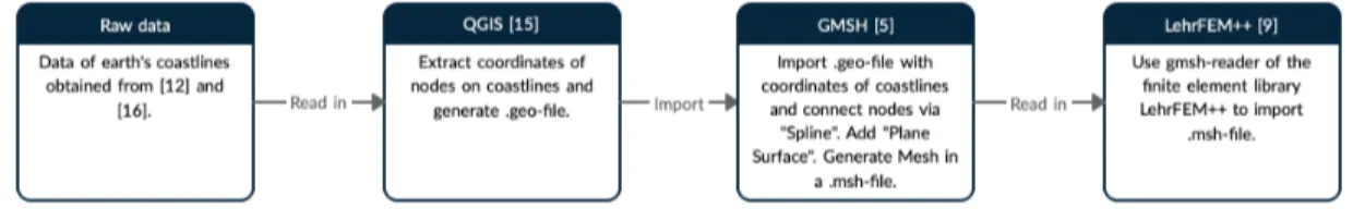
First of all, I have generated a triangulation for our domainΩ, which, in our case of popula- tion dispersal, represents the earth’s surface. The succeeding data flow diagram, figure 4.1, summarises the procedure of generating a mesh file for our domain Ω.

Figure 4.1Data flow diagram depicting the main steps to generate a triangulation of the earth’s surface.

4.1.1 Raw data

In a first step, I obtained data for the earth’s coastlines from a geographical database, main- tained by the University of Hawai’i together with a governmental geosciences lab, the national oceanic and atmospheric administration [16]. The database includes a high-resolution data set of the global shorelines. Moreover, I made use of a data base of land and sea-floor elevations [12]. This was needed to extract the contour lines of the coastlines.

4.1.2 QGIS

Subsequently, I imported this data into the geographic information system QGIS [15] via Layer → Layer hinzufügen → Vektorlayer hinzufügen. I selected the path to the data set with full resolution (GSHHS_f_L1.shp) from [16]. Furthermore, I added the data base of land and sea-floor elevations (ETOPO1_Ice_g_gmt4.grd) from [12] via Layer

→ Layer hinzufügen → Rasterlayer hinzufügen. I then extracted the contour of the coastlines, by selecting Raster → Extraktion → Kontur. Then there is the need of specifying the correct input layer (ETOPO1_Ice_g_gmt4.grd) and there is the option to save the output into a file. Also, I had to specify an additional command line argument, -fl "-200". This yields the extracted coastlines. Note that I moved the coastlines of the continents Europe, Africa and Australia to the left of America via Bearbeiten → Objekt(e) verschieben. Finally, I selected all coastlines and merged them viaBearbeiten

→ Gewählte Objekte verschmelzen. Therewith, I have now extracted the coordinates from the nodes of the shorelines.

Note that QGIS allows to install a plug-in to generate .geo-files from given input data.

This is the main reason why I have been working with QGIS. With this plug-in I was able to select Erweiterungen→ Gmsh→ Generate a Gmsh geometry file. I now selected the output file of the extracted shoreline, and then via Generate geometry file, I obtained a .geo-file with the coordinates of the nodes on all coastlines.

4.1.3 Gmsh

Consequently, I imported the resulting .geo-file into Gmsh [5]. It lists all point coordinates from nodes on the coastline. I connect these nodes by directly modifying the .geo-file: I add Spline(IL+i) = {...} where I list in curly brackets all the nodes to be connected. Note thatIL stands for the splines, whereasisimply denotes the numbering of all splines. Then I add a line loopLine Loop(ILL+i) = {IL+i}, whereILLrepresents the line loops. Finally, I add the surfaces,Plane Surface(IS+i) = {ILL+i}withISstanding for the plane surfaces.

Note that large seas inside a surface can be explicitly denoted as "holes" in the surface, by listing the corresponding line loop number denoting the surface of the "hole" behind the number of the line loop representing the surrounding surface. Furthermore, it is crucial to define the mesh size by adding these two succeeding lines on top of the .geo-file,

Mesh.CharacteristicLengthMin = 2;

Mesh.CharacteristicLengthMax = 2;

for otherwise, the resulting triangulation may be too coarse to properly respect the bound- aries.

Now I can open this modified .geo-file in Gmsh and select Mesh → 2D. This generates a two-dimensional mesh, stored in a .msh-file. Note that the number of point coordinates on the shoreline amounts to 340125. Therein are included all islands of reasonable size.

4.2 LehrFEM++

As a next step, I realised the population dispersal over the triangulated surface based on the mathematical model. The implementation heavily relies on the finite element library LehrFEM++ [9].

4.2.1 Input-Output Reader

In this library, there is a built-in reader to gather the information for the spatial mesh.

This reader extracts all necessary information from the .msh-file. The number of degrees of freedoms in the final implementation amounts to 15463. Clearly, this implies that not every node on the boundary is considered in the final mesh. This could be remedied by refining the mesh size.

4.2.2 Galerkin Matrices

In the sequel, I discuss the detailed implementation of the Galerkin matrices defined in equations (3.2), (3.3), (3.4).

For the matrix M∈R^N,N defined in (3.2), we have M:= [m(bⁱ_h, b^j_h)]^N_i,j=1 = [

Z

Ω

bⁱ_h(t,x)b^j_h(x) dx]^N_i,j=1. (4.1) This is the standard mass matrix (Remark 2.2.2.5 in [7]), and thus, I used the LehrFEM++

function ReactionDiffusionElementMatrixProviderfor its assembly.

Furthermore, for the matrix A∈R^N,N defined in (3.3), we find A:= [a(bⁱ_h, b^j_h)]^N_i,j=1 = [

Z

Ω

c(t,x) grad bⁱ_h(t,x)·grad b^j_h(x) dx]^N_i,j=1, (4.2) with diffusion coefficient c : [0, T]×Ω → R. Again, we are left with a standard Galerkin matrix, the stiffness matrix (Remark 2.2.2.5 in [7]). Thus I again made use of Reaction- DiffusionElementMatrixProvider for assembling A.

Finally, for B ∈R^N,N the discussion will be more elaborate. By definition, we obtain B := [b(bⁱ_h, b^j_h)]^N_i,j=1 = [

Z

∂Ω

Z

∂Ω

g(x,y) (bⁱ_h(t,x)−bⁱ_h(t,y))b^j_h(x) dS(y)dS(x) ]^N_i,j=1. (4.3)

We proceed by considering the two terms separately. For i, j ∈ {1, ..., N} we have B_i,j =

Z

∂Ω

Z

∂Ω

g(x,y) bⁱ_h(t,x) b^j_h(x) dS(y)dS(x)

− Z

∂Ω

Z

∂Ω

g(x,y) bⁱ_h(t,y) b^j_h(x) dS(y)dS(x)

= Z

∂Ω

Z

∂Ω

g(x,y) dS(y)bⁱ_h(t,x)b^j_h(x) dS(x)

− Z

∂Ω

Z

∂Ω

g(x,y) bⁱ_h(t,y) dS(y)b^j_h(x) dS(x) For the first integral, let us introduce the function h₁ :∂Ω→R, with

h₁(x) = Z

∂Ω

g(x,y)dS(y). (4.4)

For the second term, we introduce hⁱ₂ : [0, T]×∂Ω→R, i∈ {1, ..., N}, satisfying hⁱ₂(t,x) =

Z

∂Ω

g(x,y)bⁱ_h(t,y) dS(y), i∈ {1, ..., N}. (4.5) Then we obtain for i, j ∈ {1, ..., N},

B_i,j = Z

∂Ω

Z

∂Ω

g(x,y)dS(y)

| {z }

=: h1(x)

bⁱ_h(t,x) b^j_h(x) dS(x)

− Z

∂Ω

Z

∂Ω

g(x,y)bⁱ_h(t,y)dS(y)

| {z }

=: hⁱ₂(t,x)

b^j_h(x) dS(x)

= Z

∂Ω

h₁(x) bⁱ_h(t,x) b^j_h(x)dS(x)− Z

∂Ω

hⁱ₂(t,x) b^j_h(x) dS(x)

Now we observe that the first term corresponds to a standard mass matrix on the boundary, i.e. a mass edge matrix (Example 2.7.4.37 in [7]), with function handle h₁. Thus the implementation of theMassEdgeMatrixProviderin LehrFEM++ suits the required form.

The implementation ofh₁ requires the quadrature over∂Ω. We use theEdgeMidpointRule of third order for the concerned triangles.

The second integral demands a slightly more intricate treatment. We observe that it is of the form of a load vector (Remark 2.4.6.7 in [7]) on the boundary with function handle hⁱ₂, i ∈ {1, ..., N}. Hence we may use LehrFEM++’s ScalarLoadEdgeVectorProvider.

What concerns the function handle hⁱ₂, i ∈ {1, ..., N}, we identify again the form of a load vector, where, for fixedx∈∂Ω, we have the coefficientg depending ony∈∂Ω. This implies the use of ScalarLoadEdgeVectorProvider one more time.

The system of equations (3.15) was solved with the sparse matrix solver from the header- only library Eigen [3].

4.2.3 Visualisation

Finally, I used the VTK-writer class from LehrFEM++, to write the results into a VTK-file, which in turn I imported into ParaView [13] in order to visualise the results.

Chapter Five Model Problem

In this chapter, I discuss the simulation of equation (2.5) on simplified domains, with the aim to exhibit nice travelling wave solution as well as analysing the convergence of our numerical scheme. In the first section, we focus on travelling wave fronts.

5.1 Travelling Wave Solutions

Let me refer to section 1.1 for a discussion on travelling wave solutions. The exhibition of travelling wave fronts is taking place on three model domains.

Our first model domain is a ball of radius 0.5 around the pointy= (^0.5_0.5),

Ω˜₁ :=B_0.5((^0.5_0.5)) ={x ∈R²|kx−(^0.5_0.5)k<0.5}. (5.1) The mesh M1 for Ω˜1 is depicted in figure 5.1. We set the diffusion coefficient c and the

Figure 5.1 Triangular meshM˜1 ofΩ˜1generated with Gmsh [5].

growth factor λ to be constant. We choose a constant carrying capacity K. Furthermore, we consider homogeneous Neumann boundary conditions.

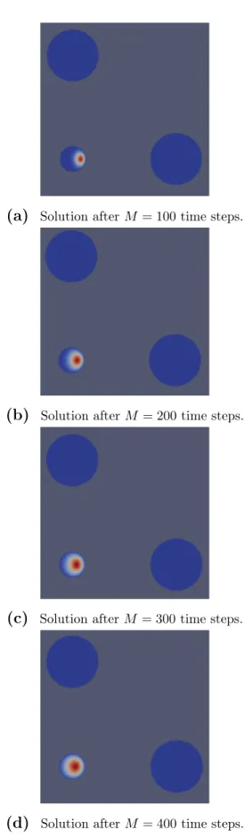
In a first step, the initial condition is represented by one point load with value 0.001 located at (_0.5¹ ). This setting yields clearly visible travelling wave fronts, originating from the initial condition, see figure 5.2.

(a) Solution after M = 100time steps. (b) Solution afterM = 200time steps.

(c) Solution afterM = 300 time steps. (d) Solution afterM = 400time steps.

Figure 5.2 Solution vector with initial condition represented by one point load visualised with ParaView [13] on mesh withN = 3581degrees of freedom.

In a second step, we leave all parameters unchanged, except for the initial condition, which is now represented by an additional point load, the first being located at (_0.5¹ ), the second located at (^0.5₁ ), both of value 0.0005. In this case we obtain again nice travelling wave fronts, originating from both sources, and superimposing one another as time evolves, see figure 5.3. Note that the wave originates from a compactly supported initial datum.

In both cases, we observe a good approximation of a wave front evolving with a finite speed of propagation. Admittedly, we must behold that in the frame of the Strang splitting, the first half time step coincides with the solution of the heat equation. Since the heat equation admits infinite speed of propagation, we expect that after this first half time step, the solution immediately attains a value arbitrarily close to zero, but non-zero, on the whole domain. This can be noticed in figure 5.10, where we can read off the values of the solution vector on the domain. There is no area where the solution is zero; instead the areas not yet populated carry values very close to zero, namely 7.1·10⁻⁶. The finite propagation speed arises due to the non-linearity. Indeed, we observe that the wave front propagates for further time steps with finite speed. Accordingly, the numerical resultsapproximate the finite speed of propagation.

Secondly, we consider three circles, at a positive distance from each other. Concretely,

(a) Solution after M = 100time steps. (b) Solution afterM = 200time steps.

(c) Solution afterM = 300 time steps. (d) Solution afterM = 400time steps.

Figure 5.3Solution vector with initial condition represented by two point loads visualised with ParaView [13] on mesh withN = 3581degrees of freedom.

we set

Ω˜₂ :=B_0.25((⁰₀))∪B_0.5((²₀))∪B_0.5((⁰₂)). (5.2) On this domain we aim to study the influence of the non-local boundary conditions (2.4) on the travelling wave solution. The mesh M˜₂ is illustrated in figure 5.4. We set the parameters as follows: we choose a constant diffusion coefficient c and growth factorλ. We set our carrying capacity K constant as well. We start with an initial population on one circle, represented by one point load of 0.00008, such that the wave front originates from this source.

In a first step, we impose homogenous Neumann boundary conditions. This yields wave fronts evolving in a single circle only, see figure 5.5. Again, the wave fronts propagate with finite speed.

In a second step, we ascertain non-local boundary conditions (2.4). The kernel is chosen as

g₁(x,y) := 1

1 +kx−yk². (5.3)

Notice that (5.3) is a slowly decaying function kernel. Note also that in this case, the kernel attributes a non-trivial value on all of the boundary∂Ω₂. With this choice, we observe that all circles are hit by the wave fronts, see figure 5.6.

Figure 5.4 Triangular meshM˜2 ofΩ˜2generated with Gmsh [5].

In a third step, we aim at further restricting the kernel. We set it to g2(x,y) :=







1

1+kx−yk², if kx−yk ≤1.75,

0, elsewhise.

(5.4)

Let me recall the domain Ω˜₂. Starting from the small ball B_0.25((⁰₀)), we realise that the upper bound kx−yk ≤1.75in (5.4) does not reach all of ∂Ω˜₂. However, we also note that an upper bound does not restrict the wave fronts from evolving along the boundaries, and thus, we still expect all of the boundary to be affected by the non-local boundary conditions.

Indeed, the results in figure 5.7 qualitatively coincide with those in figure 5.6.

Now, in a final step, we may try to confine the influence of the kernel by adding a lower bound. Consider

g₃(x,y) :=







1

1+kx−yk², if 1.25≤ kx−yk ≤1.75,

0, elsewhise.

(5.5) In compliance with Ω₂, we note that the upper bound assures that the two balls, B_0.5((²₀)) and B_0.5((⁰₂)), will be affected by the non-local boundary conditions. Nonetheless, the lower bound prevents the wave fronts to propagate along the boundaries, see figure 5.8.

As a final domain, we set Ω˜₃ to two arbitrarily shaped islands, whose boundaries are at a positive distance from each other. Figure 5.9 presents the triangular mesh M˜₃ for Ω˜₃ with 6474 degrees of freedom. In this case, the diffusion coefficient and the growth rate are chosen to be constant. The carrying capacity is constant as well. The initial condition is set to a point load having value 0.3 on the left lower corner of the right island. The decaying function kernel for the boundary conditions is chosen as in (5.3).

(a) Solution afterM = 100 time steps.

(b) Solution afterM = 200time steps.

(c) Solution after M = 300time steps.

(d) Solution afterM = 400time steps.

Figure 5.5 Solution vector with homogeneous Neumann boundary conditions visualised with

(a) Solution afterM = 100 time steps.

(b) Solution afterM = 200time steps.

(c) Solution after M = 300time steps.

(d) Solution afterM = 400time steps.

Figure 5.6 Solution vector with non-local boundary conditions using the kernel g1 visualised with ParaView [13] on M˜2.

(a) Solution afterM = 100 time steps.

(b) Solution afterM = 200time steps.

(c) Solution after M = 300time steps.

(d) Solution afterM = 400time steps.

Figure 5.7 Solution vector with non-local boundary conditions using the kernel g2 visualised with ParaView [13] on M˜2.

(a) Solution afterM = 100 time steps.

(b) Solution afterM = 200time steps.

(c) Solution after M = 300time steps.

(d) Solution afterM = 400time steps.

Figure 5.8 Solution vector with non-local boundary conditions using the kernel g3 visualised with ParaView [13] on M˜2.

Figure 5.9 Triangular meshM˜3 ofΩ˜₃generated with Gmsh [5].

In this setting, we observe in figure 5.10 the travelling wave fronts propagating with finite speed on our model domain Ω˜₃.

As a final experiment, we set the diffusion coefficient to a very small value, concretely c= 0.0625. Otherwise, we consider the same setting as above for figure 5.10; except for the growth factor λ, which we slightly decrease in order to balance the significant reduction of the diffusion coefficient. We have in mind to visualise the case where the non-local boundary conditions render the diffusion over the sea more attractive than the diffusion on land. Thus we would expect an accumulation of the solution on the boundaries ∂Ω˜₃. Let me refer to figure 5.11 which meets our expectancy. We conceive the initial datum on one island, and otherwise a distribution on the coastlines of both islands rather than a rapid diffusion on land. Nevertheless, we also observe that there is no rapid growth along the coastlines. This can be explained due to the slight decrease in the growth factor λ.

Note that in all cases, the carrying capacity represents the limit value the solutions may attain. By performing further steps in the evolution process, it can be numerically verified that the wave profiles evolve towards the stationary state whose value is given by the carrying capacity.

5.2 Convergence Analysis

This section now elucidates the convergence of the Strang splitting method applied to the initial boundary value problem (2.5). In the sequel, we consider the two arbitrarily shaped islands, Ω˜₃, as in figure 5.9.

First, remark that it is hardly possible to compute an analytical solution for problem

(a) Solution afterM = 120 time steps.

(b) Solution afterM = 240time steps.

(c) Solution after M = 360time steps.

(d) Solution afterM = 480time steps.

Figure 5.10 Solution vector visualised with ParaView [13] on mesh with N = 6474degrees of

(a) Solution afterM = 360 time steps.

(b) Solution afterM = 480time steps.

(c) Solution after M = 600time steps.

(d) Solution afterM = 720time steps.

Figure 5.11 Solution vector with a minuscule diffusion coefficient visualised with ParaView [13]

(2.5), not even in one spatial dimension, see [4]. Visually, I indeed do obtain the proclaimed travelling wave solutions, where I refer to figure 5.10. Now I aim at quantifying the conver- gence of our numerical scheme. To this end, I consider the initial boundary value problem (2.5) on the model domain Ω˜₃.

Again, I choose a constant diffusion coefficientc(t,x) =cand a constant growth factorλ.

Moreover, I choose the carrying capacity to be constant as well. As this capacity represents the maximal limit value for the population density, I expect the solution to attain this limit after a sufficiently long evolution. Furthermore, the same kernel g is chosen as in (5.5) with adequate bounds to account for the non-local boundary values. Finally, the initial population is again represented by a point load on one of the islands.

I perform three different convergence analyses. Firstly, I control the error with the mesh size. Secondly, I govern the error in the time step sizes; and lastly, I consider the solution by regulating both, the mesh width and the time step size synchronously, see section 6.2.8 in [7].

5.2.1 Convergence Studies for Mesh Width

I generate an initial mesh on the model domainΩ˜₃, having in this case39degrees of freedom, and refine it with LehrFEM++’sMesh Hierarchy class in the namespace refinement[9].

The finest mesh has6474degrees of freedom. Since no analytic solution is available, I instead refer to the solution on the finest mesh, see figure 5.12. I let the time step size be constant (i.e. τ = 0.01), small enough to measure the discrete error in the mesh size. In figure 5.12, the L²( ˜Ω₃)-norm of the difference of the solution on the considered mesh and the solution on the finest mesh is computed; that is

(e)_l:=p

h(l)ku_N(l)−u_N(5)k_L2( ˜Ω3), l ∈ {1, ...,4}, (5.6) whereu_N(l), l ∈ {1, ...,5}represents the discrete solution vector on a mesh withN(l)degrees of freedom after 100 time steps, and where h∈ R denotes the mesh width. Note that N(l) is given by

N(1) = 39, N(2) = 125, N(3) = 444, N(4) = 1670, N(5) = 6474.

Also notice that we have to interpolate the solution vectors in the finite element setting u_N(l), l ∈ {1, ...,4} onto the finest mesh with N(5) = 6474 degrees of freedom such that the difference in (5.6) is well-defined. This is done with LehrFEM++’s MeshFunctionFE-, MeshFunctionTransfer- andNodalProjection-functionality [9]. Concretely, this means that we consider the solution vectors on the coarse meshes withN(l), l∈ {1, ...,4}degrees of

freedom. For these we then extract the corresponding mesh functions using theMeshFunc- tionFE-functionality. The result is transferred onto the finest mesh via MeshFunction- Transfer. Finally, with theNodalProjection-functionality we obtain the solution vectors u_N(l), l∈ {1, ...,4} interpolated onto the finest mesh.

10² 10³

Number of degrees of freedom 10^-1

10⁰ 10¹

L2 error with respect to solution on finest mesh

L2 error slope: -1.12

(a) L²( ˜Ω3)-norm against number of degrees of freedom N.

0.5 1 1.5 2 2.5 3 3.5

Mesh Width h 10^-1

10⁰ 10¹

L2 error with respect to solution on finest mesh

L2 error slope: 2.02

(b) L²( ˜Ω₃)-norm against mesh sizeh.

Figure 5.12 L²( ˜Ω3)-norm of difference of final solution after100 time steps on meshes with number of degrees of freedomN ∈ {39,125,444,1670,6474} with respect to the final solution on the finest mesh withN = 6474degrees of freedom.

We observe an algebraic convergence rate of 1.12 in terms of the number of degrees of freedom for the Strang splitting method, and thus an algebraic rate of convergence of 2.02 in terms of the mesh size. Therefore, the error behaves asymptotically as O(N) = O(h²), where h denotes the mesh width.

5.2.2 Convergence Studies for Time Step Sizes

In this section, I instead govern the time step sizes to analyse the incurred error. To this end I consider a sufficiently fine mesh M₃ for Ω˜₃ with 1670 degrees of freedom. I consider different number of time steps M, namely

M(1) = 10, M(2) = 20, M(3) = 40, M(4) = 80, M(5) = 160, M(6) = 320.

The time step sizesτ(l) = _M(l)^T , l∈ {1, ...,6} for final time T = 1 are then correspondingly, τ(1) = 0.1, τ(2) = 0.05, τ(3) = 0.025,

τ(4) = 0.00125, τ(5) = 0.000625, τ(6) = 0.0003125.

Again, having no analytical solution at hand, I instead refer to the solution computed with the smallest time step sizeτ(6) = 0.0003125. I then control theL²( ˜Ω₃)-norm of the difference of the solutions u_M(l), l ∈ {1, ...,5} and the solution with most time steps, u_M(6). In figure 5.13, you observe

(e)_l:=p

τ(l)ku_M(l)−u_M(6)k_L2( ˜Ω3), l∈ {1, ...,5}, (5.7) plotted against the number of time steps M(l), l ∈ {1, ...,5}. There is an algebraic rate of convergence of −1.7, and thus an asymptotic behaviour of O(M^−1.7) = O(τ^1.7). Theoreti- cally, we would expect a convergence rate of O(τ²), for the employed SDIRK method is of order 2, and for the reaction term we have applied an exact evolution operator.

5.2.3 Convergence Studies for Mesh Width linked to Time Step Sizes

Finally, we link the mesh sizes to the time step sizes, and control the error norm incurred thereof.

In theory, the error norm behaves as O(h² +τ²). Thus, we impose a linear dependence of mesh width to time step size. Concretely, we consider different meshes refined as above for N ∈ {39,125,444,1670,6474} degrees of freedom. We start with M(1) = 100 number of time steps. For l ∈ {2, ...,5} we set

τ(l) = τ(1)

h(1)h(l), (5.8)

where h(l) is the mesh size for the mesh with N(l) degrees of freedom. The corresponding number of time steps M(l) are rounded to the next integer,

M(l) = d T

τ(l)e, l∈ {2, ...,5}, (5.9)

10¹ 10² Number of time steps

10^-4 10^-3 10^-2

L2 error with respect to solution of smallest time step size

L2 error slope: -1.7

(a) L²( ˜Ω3)-norm against number of time stepsM.

10^-2 10^-1

Time step size 10^-4

10^-3 10^-2

L2 error with respect to solution of smallest time step size

L2 error slope: 1.7

(b) L²( ˜Ω₃)-norm against time step sizeτ.

Figure 5.13 L²( ˜Ω3)-norm of difference of final solutions with number of time steps M ∈ {10,20,40,80,160,320} with respect to M(6) = 320 time steps on a mesh with N = 1670 de- grees of freedom.

with final time T = 1.

Let me refer to figure 5.14, which illustrates (e)_l:=p

h(l)ku_N(l),M(l)−u_N(5),M(5)k_L2( ˜Ω3), l ∈ {1, ...,4}, (5.10) whereu_N(5),M(5) is the reference solution on the finest mesh. Again, let me point out that the solution on the coarser meshesu_N(l),M(l), l∈ {1, ...,4}, were interpolated onto the finest mesh using LehrFEM++’s functionalities as above in section 5.2.1. We conceive the asymptotes O(N +M²) = O(h²+τ²), as predicted.