Automated Planning of Process Models:
Design of a Novel Approach to Construct Exclusive Choices
Authors:
Heinrich, Bernd, Department of Management Information Systems, University of Regensburg, Universitätsstrasse 31, D-93040 Regensburg, Germany, bernd.heinrich@ur.de
Mathias, Klier, Department of Management Information Systems, University of Regensburg, Universitätsstrasse 31, D-93040 Regensburg, Germany, mathias.klier@ur.de
Steffen Zimmermann, Department of Information Systems, Production and Logistics Management, University of Innsbruck, Universitätsstrasse 15, A-6020 Innsbruck, Austria,
Steffen.Zimmermann@uibk.ac.at
Citation: Bernd Heinrich, Mathias Klier, Steffen Zimmermann, Automated Planning of Process Models: Design of a Novel Approach to Construct Exclusive Choices, Decision Support Systems, Volume 78, October 2015, Pages 1–14, ISSN 0167-9236, http://dx.doi.org/10.1016/j.dss.2015.07.005.
(http://www.sciencedirect.com/science/article/pii/S0167923615000299)
Automated Planning of Process Models:
Design of a Novel Approach to Construct Exclusive Choices
Abstract
In times of dynamically changing markets, companies are forced to (re)design their processes quickly and frequently, which typically implies a significant degree of time-consuming and cost-intensive manual work. To alleviate this drawback, we envision the automated planning of process models. More precisely, we propose a novel algorithm for an automated construction of the control flow pattern ‘exclusive choice’, which constitutes an essential step toward an automated planning of process models. The algorithm is built upon an abstract representation language that provides a general and formal basis and serves as the vocabulary to define the planning problem. As part of our evaluation, we find that, based on a given planning problem, our algorithm is not subject to potential modeling failures. We further implement the approach in process planning software and analyze not only its feasibility and applicability by means of several real-world processes from different application contexts and companies but also its practical utility based on the criteria flexibility by definition, modeling costs, and modeling time.
Keywords: process model; automated planning; exclusive choice; algorithm; design science research
1. INTRODUCTION
In times of dynamically changing markets, companies must frequently (re)design their business processes to adapt them to new market conditions such as shifting customer needs and new offers of emerging competitors.
At the same time, companies are increasingly embedded in interorganizational, process-based collaborations, a fact that makes process (re)designs all the more complex. For instance, we are involved in an extensive project including several process (re)designs with a European bank in which over 600 core business processes and 1,500 support processes are modeled in different departments and areas. These process models, which are composed of actions and corresponding control flows [33], are modeled using the ARIS toolset and documented in a company-wide process repository to support the standardization of processes and to have a common base for process (re)design projects. To keep the process models updated, it is necessary to frequently (re)design process models due to changing market conditions such as new products, new distribution channels, and new regulatory obligations. Several interviews with IT and business executives of the bank highlighted the fact that today’s process (re)design projects are more cost-intensive and time-consuming than such projects
were 10 years ago due to their higher complexity. This change also became evident in interviews with executives of other branches such as insurance and engineering. The most frequently mentioned reasons for increasing costs and duration are the growing frequency and complexity of such process (re)design projects, which involve a significant degree of manual work (cf. also [32]).
The research strand of Semantic Business Process Management (SBPM) aims to alleviate this drawback by using semantic technologies to enable a higher level of automation when designing, processing, executing, and analyzing processes and process models [26]. Wetzstein et al. [58] structure the scope of SBPM in their SBPM lifecycle and differentiate four phases: SBP modeling, SBP implementation, SBP execution, and SBP analysis.
In our research, we aim to contribute to SBP modeling. The objectives in this phase are the semantic annotation, the design, and the adaptation of process models in an automated manner and their evaluation to ensure feasibility and (practical) utility [58].
Focusing on the SBP modeling phase, we envision the automated planning of process models. We aim to develop a planning approach that automatically arranges semantically annotated actions in a control flow leading from an initial state to desired goal states. When applying such an approach, the (re)design of process models is no longer performed manually but by an algorithm that uses semantic concepts and automated reasoning. With this research, we aim to increase the flexibility by definition (cf. [49]) of the resulting process models and to (re)design process models - for processes that must be frequently (re)designed – to be more cost- efficient and less time-consuming compared with manual process modeling. For automated process planning, it is insufficient to construct sequences of actions because entire process models include control flow patterns [43]. The specific research goal of this paper is the automated construction of one of the most important control flow patterns, namely exclusive choice.
Therefore, we initially define an abstract representation language to express the preconditions (comprising everything an action requires to be applied, including input parameters) and effects (how an action affects the state of the world, including output parameters) of actions and belief states (possibly infinite sets of world states that may exist before and after applying an action). Using this abstract representation language, we define our planning problem and, most importantly, design a novel algorithm for the automated construction of exclusive choices. As part of the evaluation, we find that, based on a given planning problem, our algorithm is not subject to potential modeling failures. We further implement the approach in SBPM process planning software and analyze not only its feasibility and applicability by means of several real-world processes but also its practical
utility based on the criteria flexibility by definition, modeling costs, and modeling time.
The research presented in this paper is based on the Design Science Research paradigm [18, 27]. In the introduction, we motivated the research problem - the automated construction of exclusive choices. In Section 2, we discuss contributions addressing related research problems (prescriptive knowledge) and elaborate the research gap. In Section 3, we present a general approach for an automated planning of process models to inform our research problem (descriptive knowledge). In section 4, we introduce a running example to illustrate the basic idea of our approach as well as each design step in the remainder of the paper. In Section 5, we present our approach for an automated construction of exclusive choices. Section 6 is dedicated to the evaluation of our approach. In Section 7, we discuss limitations and directions for future research before we conclude with a summary of our key findings in Section 8.
2. RELATED LITERATURE
Works addressing research problems that are related to the automated construction of exclusive choices are found in the research fields of Automated Planning and SBPM. Beginning with the literature in Automated Planning, the planning problem addressed in this paper can be characterized as a nondeterministic planning problem with initial state uncertainty. Algorithms that can cope with nondeterminism and initial state uncertainty [4, 8, 28] are called conditional planning approaches. When constructing exclusive choices in process models, an approach must cope with large data types (e.g., double) and possibly infinite sets of world states. However, according to Geffner [15], a key problem in large state spaces – resulting from large data types and possibly infinite sets of world states – is representing belief states and enabling mapping of one belief state onto another. In this context, Bertoli et al. [4] propose the use of Binary Decision Diagrams. Another possibility is the implicit representation of a belief state by an initial state in combination with a sequence of actions that leads to the belief state to be represented [29]. Further planners explicitly enumerate all world states that may occur after applying an action [7]. However, in the context of planning process models and constructing exclusive choices, it is essential to cope with large data types accompanied by infinite sets of world states. This issue has not thus far been addressed by existing approaches. Moreover, existing conditional planning approaches operate with so-called observations, which are points in the plan at which it is necessary to validate some logical expression to define how to proceed. However, these observations are encoded separately in the form of observation variables and observation actions making them both part of the given planning domain.
Here, the observations in the domain description constitute the only points in the plan in which the control flow
might branch (e.g., to construct exclusive choices). Thus, it is possible to consider exclusive choices using existing conditional planners [8, 28], but they must be “hard-coded” in the domain (e.g., by sensing actions) and are additionally restricted to Boolean variables. However, in the context of planning process models, the points in the plan at which exclusive choices appear are not given; rather the corresponding conditions for which the control flow branches must be planned considering large data types. This challenge has so far also not yet been addressed by existing planning approaches.
In addition to the literature on Automated Planning, we discuss related approaches in the field of SBPM structured according to the phases of the SBPM lifecycle by Wetzstein et al. [58]:
SBP analysis: This phase comprises process mining and the validation of existing process models. The goal of process mining algorithms is to deduce process models from event logs representing recorded information about (many) former executions of the considered process [50, 52]. The deduced process models can then be compared with the deployed process models and thus be used for conformance checking and optimization purposes [53]. Existing process mining algorithms are able to identify control flow patterns based on dependency relationships observed in the event logs [3, 14, 17, 50, 51, 56, 57]. However, because these approaches focus on dependencies among actions, they do not aim at deriving the conditions of exclusive choices, which is an indispensable step toward our goal of planning exclusive choices in process models.
Moreover, to derive the conditions of exclusive choices in the case of large data types, the event log would have to contain information about a possibly infinite number of process executions, which is rather unrealistic.
Another major difference between process mining and the automated planning of process models refers to the fact that process mining aims at reconstructing models for as-is processes to capture the processes as they are actually being executed [57]. In contrast, the automated planning of process models focuses on the construction of to-be process models for a given planning problem. Further related work in the SBP analysis phase aims at examining the consistency of existing process models [13, 34, 55]. These approaches validate whether the actions (within a process model) are consistent both among themselves and with respect to the control flow patterns used. Thus, they check whether exclusive choices are consistently constructed in given process models but do not focus on elaborating a planning domain or an algorithm to construct exclusive choices.
SBP implementation and execution: Within these phases, (web) services that are required to execute processes are composed in an automated manner. For that purpose, multiple service composition approaches were developed in recent years that are motivated by a problem definition related to planning process models
[1, 5, 6, 11, 30, 36, 37, 38, 40, 42, 45, 46, 48, 54, 59] (for a current overview of research on web service composition see e.g., [44]). However, few of them consider conditions that are required to construct exclusive choices. For instance, Meyer and Weske [38] propose to extend an enforced Hill-Climbing algorithm to support the construction of alternative control flows. They add an or-split to the service composition “if subsequent services cannot be invoked in all states”. However, they do not consider belief states able to consider possibly infinite sets of world states. Bertoli et al. [6] (and other authors such as Wu et al. [59]) propose a planning framework to create a composite service that can handle services specified and implemented using industrial standard languages for business process execution. However, they do not focus on planning conditions for exclusive choices but on identifying one feasible service composition based on a search tree. Wang et al. [54]
aim at integrating conditional branch structures in automated web service composition to represent users’
diverse and personalized needs in combination with dynamic environmental changes. They propose algorithms that are based on formalized user preferences (e.g., P = AccountBalance Payment? – PayInFull:
PayByInstalments; i.e., the user will pay in full, if (s)he has sufficient money; otherwise, (s)he will pay by instalments). These preferences are explicitly specified and given as part of the web service composition problem. Therefore, in contrast to constructing exclusive choices and conditions, the approach of Wang et al.
[54] somehow predefines the points at which the control flow might branch (e.g., to construct an exclusive choice) and the corresponding conditions in the problem definition.
SBP modeling: This phase is about the automated construction of process models but has thus far been much less extensively researched compared with the other phases. Hoffmann et al. [31] aim at leveraging synergies with model-based software development and propose a heuristic that can be used to reduce additional modeling overhead caused by planning process models. They adapt a well-known deterministic planning system to allow for nondeterministic actions that are characterized by multiple possible disjunctive effects predefined using finite-domain variables. Based on predefined possible effects and corresponding case distinctions (one case for each possible outcome), exclusive choices can be defined after a nondeterministic action. However, Hoffmann et al. [31] aim at deriving neither the partitions (conditions) of exclusive choices nor multiple feasible process models differing in their exclusive choices. Other approaches that are associated with the SBP modeling phase do not address the construction of exclusive choices.
In summary, to the best of our knowledge, none of the existing approaches aims to cope with the following set of necessary characteristics when constructing exclusive choices in process models:
(1) Consider large data types and possibly infinite sets of world states;
(2) Construct exclusive choices in an automated manner without “hard-coded” observations in the given planning domain by creating partitions and corresponding conditions;
(3) Construct multiple feasible process models (feasible solutions) differing in their exclusive choices; and (4) Construct exclusive choices in to-be process models in an automated manner.
Thus, we address an important research gap by constructing exclusive choices and enabling the planning of all feasible process models for a specific planning problem in an automated manner.
3. AUTOMATED PROCESS PLANNING APPROACH
The automated construction of exclusive choices is necessary but not sufficient to plan entire process models.
Therefore, we started to design a planning approach of which the proposed algorithm to construct exclusive choices constitutes a fundamental part. Our planning approach is based on semantically annotated actions stored in an action library. The annotation of an action includes a semantic annotation of its logical preconditions and effects. In addition to the annotated actions, our starting point comprises an initial state representing the overall process input and one or more goal states representing the necessary process output.
Thus, our planning approach constructs feasible process models in an automated manner. The three steps to
of the planning approach include the following:
Semantic-based reasoning of dependencies between actions: To identify dependencies between actions, we use semantic reasoning. In other words, we analyze the semantic matching between preconditions and effects of actions in the action library. The dependencies are represented in a Dependency Graph. To construct this graph and exclude actions that cannot be part of feasible process models (feasible solutions), we apply a backward search algorithm starting from the goal state(s) and ending in the initial state.
Planning feasible sequences of actions: The Dependency Graph describes no direct predecessor-successor- relationships among actions. Hence, in the second step, a forward search algorithm is applied to determine all sequences of actions leading from the initial state to the goal state(s). Thus, we obtain a Search Graph that is an acyclic, bipartite directed graph and comprises all feasible sequences of actions for the corresponding planning problem.
Construction of control flow patterns and feasible process models: To obtain process models (e.g., UML Activity Diagrams), planning only sequences of actions such as those represented by the Search Graph is insufficient. Rather, in the third step, control flow patterns [43] provided by process modeling languages
and describing the control flow must be constructed in an automated manner [21].
In the literature, there are approaches that can serve as an initial basis to design algorithms that address the steps of our planning approach. Concerning the semantic-based reasoning of dependencies between actions (cf.
step ), existing approaches that are also used in web service composition can be considered [20, 23]. To plan feasible sequences of actions (cf. step ), existing planning techniques [4, 8, 28] can be enhanced [25]. The construction of control flow patterns and feasible process models based on a Search Graph (cf. step ) is especially challenging and innovative. In this step, the automated construction of exclusive choices is essential.
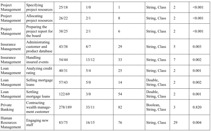
This is supported by our analyses of several processes from different application contexts and companies (cf.
Section 6). Indeed, we found that all considered processes contain one to many simple and nested exclusive choices, which illustrates the importance of exclusive choices for specifying the control flow in process models.
4. RUNNING EXAMPLE
The example is taken from the security order management of a European bank. We will illustrate our approach and each design step based on an excerpt of the order execution process that is part of the core business of the bank. In the past, this process had to be frequently (re)designed due to repeated launches of new products and regulations. The actions validate order, assess risks, check competencies, check extended competencies, and execute order, which are part of the excerpt of the process, are available in the library. In the initial state, an order is entered by a customer with the parameters orderAmount that may reach from 0 to 250,000, orderState with the value entered, and orderType with the feasible values buyOrder and sellOrder. In the goal state, the order must be executed (executed is the required value for the parameter orderState).
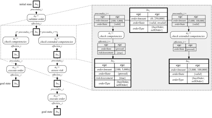
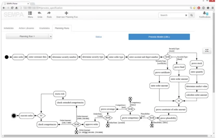
Applying a version of the well-known forward search algorithm of Bertoli et al. [4], which is implemented in our SBPM process planning software (cf. Section 6.2), results in the Search Graph depicted in Figure 1. This graph was chosen to ensure a sound and established general basis, which is also used by other approaches, for instance in the field of web service composition. The Search Graph is an acyclic, bipartite directed graph with a set of nodes and a set of labeled arcs. The set of nodes consists of actions (e.g., check competencies) and belief states (e.g., bs1). The arcs are labeled with the preconditions (e.g., precond(check competencies)) and effects (e.g., effects(check competencies)) of the corresponding actions. Containing all sequences of actions leading from the initial state to the goal state(s), this graph provides a sound basis for constructing exclusive choices.
Fig. 1. Search Graph for constructing exclusive choices
For brevity, we only present in detail the part of the Search Graph in the dashed rectangle. In belief state bs1, the action validate order has already been applied. Therefore, the parameter orderState is assigned either of the values valid or invalid (in contrast to entered in the initial state). In bs1, it is necessary to decide which check routine to apply. In this context, the preconditions specified for the actions must be considered. The actions check competencies and check extended competencies are applicable to orders with an orderAmount between 100 and 5,000 and between 3,000 and 100,000, respectively. Both actions require orderState valid and result in orderState proved. Because the action check competencies comprises a lean risk assessment that is sufficient for orders with an orderAmount between 100 and 5,000, the effects of this action additionally contain the parameter riskAssessment with the value true. Thus, planning the action check competencies after belief state bs1 leads to belief state bs2. In contrast, the action check extended competencies does not comprise a simple risk assessment. Rather it is necessary to conduct a more comprehensive risk assessment by a separate action assess risk. Thus, planning the action check extended competencies after belief state bs1 leads to belief state bs3. This excerpt of the entire order execution process serves as a running example to illustrate our design steps.
5. NOVEL APPROACH TO CONSTRUCT EXCLUSIVE CHOICES
To design our approach, we initially specify an abstract representation language. Using this language, we define our planning problem and design an algorithm to construct exclusive choices.
effects(a3,2) a3,2:=
execute order
precond(a1):=
v(p) r(p)
orderAmount [100; 5,000]
orderState {valid}
bs2
v(p) r(p)
orderAmount [100; 5,000)]
orderState {proved}
riskAssessment {true}
orderType {buyOrder, sellOrder}
bs3
v(p) r(p)
orderAmount [3,000; 100,000]
orderState {valid}
orderType {buyOrder, sellOrder}
a1:=
check competencies
bs1
v(p) r(p)
orderAmount (0; 250,000]
orderState {valid,invalid}
orderType {buyOrder, sellOrder}
a2:=
check extended competencies precond(a2):=
v(p) r(p)
orderAmount [3,000; 100,000]
orderState {valid}
effects(a2):=
v(p) r(p)
orderState {proved}
effects(a1):=
v(p) r(p)
riskAssessment {true}
orderState {proved}
bs0
bs4
bs6
initial state precond(a0) precond(a0)
effects(a0) a0:=
validate order
precond(a0) precond(a4)
effects(a4) a4:=
assess risk precond(a0)
precond(a3,1)
effects(a3,1) a3,1:=
execute order
precond(a3,2) precond(a1) precond(a2)
effects(a1) effects(a2)
a1:=
check competencies a2:=
check extended competencies bs1
bs3
bs5
goal state
goal state
5.1 Specifying an Abstract Representation Language
In this subsection, we present an abstract representation language for planning process models. Classical planners, which use other representation languages such as set-theoretic representation or state-variable representation [16], usually consider a finite set of world states and enumerate, for instance, all world states that may occur after applying an action explicitly [7]. This is not possible in the context of planning process models.
Here, we must consider large data types and possibly infinite sets of world states. However, if we restrict all of the atoms and belief state variables to be ground, then from a theoretical point of view, our abstract representation language has equivalent expressiveness compared to the other languages mentioned. Our abstract representation language does not depend on any concrete process modeling language but provides a general and formal basis and serves as vocabulary to describe our planning problem and design our artifact.
When talking about process models, the annotation of their actions includes a specification of the preconditions and the effects. We define a parameter of the preconditions and effects as belief state tuple that consists of the parameter’s name and a subset of its predefined domain containing all values that can be assigned to the parameter in a specific world state (corresponding to an individual process execution). Thus, the name of a parameter is also understood as a variable that can take all values in the specified subset. The data type of a parameter is the predefined domain of a belief state tuple.
Definition 1 (Belief state tuple). A belief state tuple p is a tuple of a belief state variable v(p) and a subset r(p) of its predefined domain dom(p), which we will write as p := (v(p), r(p)). It is v(p) r(p) in a specific world state. When talking about belief states, v(p) is the symbol of the belief state variable. The set r(p) dom(p) defined by logical and set-theoretic expressions is called the belief-state-variable restriction (abbr.: restriction) of v(p), which contains all of the values that can be assigned to v(p) in a specific world state. If r(p) = then the belief state variable does not exist (anymore), allowing its deletion.
According to this definition, each belief state variable v(p) has a predefined data type specifying the domain dom(p) (e.g., dom(orderAmount) = double). Additionally, the restriction r(p) can be defined for each belief state variable v(p). A restriction can either be described by logical expressions (e.g., r(orderAmount) = {x | x dom(orderAmount) 100 <x 5,000} = (100; 5,000]) defining a set of values or an explicit enumeration of discrete values (e.g., r(orderState) = {valid, invalid}) for a specific belief state variable.
Example 1 illustrates the definition of belief state tuples in bs1 of our running example.
Example 1. bs1 = {(orderAmount, (0; 250,000]), (orderState, {valid, invalid}), (orderType, {buyOrder,
sellOrder})} represents a set of belief state tuples. The restriction of orderAmount is an interval of the double data type, whereas 0 is not part of the interval but 250,000 is. The domains of the belief state variables are predefined as dom(orderAmount) = double, dom(orderState) = {entered, valid, invalid, proved, executed}, and dom(orderType) = {buyOrder, sellOrder}.
By using belief state tuples, we can represent belief states and describe in what sense we understand them as possibly infinite sets of world states with the help of Definition 3 in combination with Definition 2.
Definition 2 (⋿). Let A = {u1, …, uk} and B = {w1, …, wm} be two finite sets of belief state tuples. Then A ⋿ B : w B u A: v(w) = v(u) r(u) r(w) |r(u)|=1.
Definition 3 (Belief state and world state). Let BST = {p1, …, pn} be a finite set of belief state tuples. A belief state bs is a subset of BST, containing every belief state variable one time at most (i.e., pi, pj bs, pi pj: v(pi) v(pj)). A world state s is a member of a belief state bs, in the context that s ⋿ bs.
According to Definition 3, a belief state bs is characterized by a finite set of pairwise distinct belief state variables and their restrictions (i.e., bs BST = {p1, …, pn} pi, pj bs, pi pj: v(pi) v(pj)). Similar to Petrick and Bacchus [41], set bs can be interpreted as a type of knowledge base capturing the knowledge about available belief state variables v(pi) including the values r(pi) that can be assigned to these variables in a specific world state. In contrast to a world state – which generally refers to an individual process execution – bs describes different conceivable world states. Indeed, bs is a set of world states whereby in a world state s of belief state bs (i.e., s ⋿ bs), each belief state variable v(pi) in bs is available and is assigned a specific concrete value which satisfies the corresponding belief state variable restriction r(pi) (cf. Definition 2). According to the literature [4, 7, 28, 29], a set of world states is called a belief state. Definition 3 follows this wording.
This means of representing a set of world states is the starting point to define our planning problem.
Furthermore, we can explicitly represent belief states intuitively from a process modeling perspective.
Additionally, with this representation language, a belief state can be a possibly infinite set of world states.
5.2 Specifying the Planning Problem
Our planning problem can be considered as a nondeterministic planning problem with initial state uncertainty.
The theoretical basis for our approach is the framework given in Bertoli et al. [4]. However, we will describe our domain using the abstract representation language specified in Subsection 5.1 to allow the consideration of data types accompanied by possibly infinite sets of world states and to handle nondeterminism differently.
Furthermore, Bertoli et al. [4] explicitly assume given observationsfor which the control flow might branch on conditions as part of the problem domain. Thus, the observations and the corresponding conditions must be known in advance. Because this is not realistic in the context of process modeling, we must develop our own approach to make it possible to identify these points in the plan and to create conditions under which the plan branches (i.e., exclusive choice) in an automated manner.
In this subsection, we describe our design process, beginning with a nondeterministic state-transition system and its definition (Starting Point). To be able to cope with possibly infinite sets of world states, we modify and extend this definition. Instead of states, we use belief states in the transition system, which makes it possible to change the transition function to be deterministic concerning belief states. This approach results in the definition of a deterministic belief-state-transition system (First Step). To be able to build branches in the plan, we further extend the transition function by conditions and define our planning domain as a conditional deterministic belief-state-transition system (Second Step). Finally, the planning domain, in combination with the initial state and the goal states, represents our planning problem (Third Step).
5.3 Starting Point: Nondeterministic State-Transition System by Bertoli et al. [4]
When confronted with a nondeterministic planning problem, it is common to use a nondeterministic planning domain. In general, “a nondeterministic state-transition system is defined in terms of its states, its actions, and a transition function that describes how (the application of) an action leads from one state to possibly many states” [4]. We use this as a working definition of a nondeterministic state-transition system. More precisely, a state-transition system and (non)determinism in state space are defined as follows [4].
Definition 4 (Nondeterministic state-transition system). “A nondeterministic state-transition system is a tuple
= (S, A, R), where
S is a finite set of states,
A is a finite set of actions, and
: S × A → 2S is the transition function. The transition function associates to each state s S and to each action a A the set (s, a) S of next states.”
Definition 5 ((Non-)determinism in state space). “An action a is applicable in a state s ([…]) iff |(s, a)| > 0; it is deterministic (nondeterministic) in s iff |(s, a)| = 1 (|(s, a)| > 1). If a is applicable in s, then (s, a) is the set of states that can be reached from s by applying a.”
As mentioned, we take this nondeterministic state-transition system as a starting point and modify and extend it to be able to cope with possibly infinite sets of world states.
5.3.1 First Step: Definition of a Deterministic Belief-State-Transition System
We defined a nondeterministic state-transition system and what we understand as a belief state. On this basis, we define a deterministic belief-state-transition system and determinism in belief space. Our transition system is called a belief-state-transition system because it is not based on states but on belief states. Similar to the nondeterministic state-transition system, we formulate a working definition of a deterministic belief-state- transition system that is defined in terms of its belief states (sets of world states), its actions, and a transition function that describes how (applying) an action leads from one belief state to one and only one belief state.
Definition 6 (Deterministic belief-state-transition system). A deterministic belief-state-transition system is a tuple d = (BS, A, d), where
BS is a finite set of belief states,
A is a finite set of actions, and
d : BS × A → BS is the transition function. The transition function associates to each belief state bs BS and to each action a A the next belief state d(bs, a) BS.
Definition 7 (Determinism in belief state space). An action a is deterministic in a belief state bs iff
|d(bs, a)| = 1. If a is applicable in bs, then d(bs, a) is the set of belief states that can be reached from bs by applying a.
According to Definition 7, the belief-state-transition system in Definition 6 is called deterministic because its transition function associates to each belief state bs BS and to each action a A the next belief state
d(bs, a) BS. Therefore, |d(bs, a)| = 1 holds for each action a that is applicable in bs. This deterministic belief-state-transition system allows transitions from a set of world states to a set of next world states, which is made possible through using belief states. Hence, the nondeterministic state-transition system is extended to allow transitions from one world state to a set of next world states. In addition, belief states may represent possibly infinite sets of world states. Consequently, the deterministic belief-state-transition system extends the nondeterministic state-transition system, which can only cope with finite sets of world states.
Based on Definition 6, we define our planning domain as a deterministic belief-state-transition system
d = (BS, A, d). To do so, we must specify the finite set of belief states BS, the finite set of actions A, and the
transition function d : BS × A → BS, which associates to each belief state bs BS and to each action a A the next belief state d(bs, a) BS. First, we provide some basic definitions.
Definition 8 (Action). Let BST = {p1, …, pn} be a finite set of belief state tuples. An action a is a triple consisting of the action name and two subsets of BST, which we will write as a := (name(a), precond(a), effects(a)). Here, precond(a) BST denotes the preconditions, and effects(a) BST denotes the effects of a, both containing each belief state variable one time at most (i.e., pi, pj precond(a), pi pj: v(pi) v(pj) and pi, pj effects(a), pi pj: v(pi) v(pj), respectively).
Definition 9 (). Let A = {u1, …, uk} and B = {w1, …, wm} be two finite sets of belief state tuples, both containing each belief state variable one time at most (i.e., ui, uj A, ui uj: v(ui) v(uj) and wi, wj B, wi wj: v(wi) v(wj), respectively). Then
A B : w B u A: v(w) = v(u) r(u) r(w).
Definition 10 (Applicable). Let bs be a belief state and a an action. Then, action a is applicable in belief state bs (denoted with applicable(a, bs)) iff bs precond(a).
Definition 10 phrases a sufficient condition that must be met so that an action a can actually be applied in all possible world states of a belief state bs. All belief state variables in precond(a) are available in bs. At the same time, the restriction of each belief state variable in bs is a subset of the restriction required by a belief state variable in precond(a). In other words, an action is applicable iff the action can be applied in each world state s ⋿ bs. On this basis, we define a deterministic belief-state-transition system.
Definition 11 (Deterministic belief-state-transition system). Let BST = {p1, …, pn} be a finite set of belief state tuples. We define our planning domain as a deterministic belief-state-transition system d = (BS, A, d), where
BS 2BST is a finite set of belief states (i.e., each belief state bs BS is a subset of BST),
A is a finite set of actions, where precond(a) BST and effects(a) BST for each a A, and
d : BS × A → BS is the transition function that associates to each belief state bs BS and to each action a A the next belief state d(bs, a) BS as follows: d(bs, a) = {(bs \ {(vbs, rbs) | (vbs, rbs) bs (veffects, reffects) effects(a) vbs = veffects}) effects(a)} if applicable(a, bs), and otherwise.
BS is closed under d, i.e., if bs BS, then for each belief state, bs BS, and each action a A, d(bs, a) BS holds (Definition 6).
Example 2 illustrates the deterministic belief-state-transition system for the application of the action check
competencies in bs1 of our running example.
Example 2. Let (a1 := check competencies, precond(a1) := {(orderAmount, [100; 5,000]), (orderState, {valid})}, effects(a1) := {(orderState, {proved}), (riskAssessment, {true})}) be an action and let bs1 = {(orderAmount, [1,000; 3,000]), (orderState, {valid}), (orderType, {buyOrder, sellOrder})} be a belief state. a1 is applicable in bs1, since bs1 precond(a1) because for each variable among the preconditions of a1 there is a variable in bs1 and it is [1,000; 3,000]orderAmount_bs1 [100; 5,000]orderAmount_a1, {valid}orderState_bs1 {valid}orderState_a1. As a result it is d(bs1, a1) = {{(orderAmount, [1,000; 3,000]), (orderState, {proved}), (riskAssessment, {true}), (orderType, {buyOrder, sellOrder})}}.
5.3.2 Second Step: Definition of a Conditional Deterministic Belief-State-Transition System
In the deterministic belief-state-transition system of Definition 11, a transition can only occur if an action is applicable for all world states of a belief state. Therefore, the transition function d might leave out transitions that are typical in the process modeling context. To illustrate this problem, compared with Example 2 we change the restrictions of belief state variables orderAmount and orderState of bs1 (cf. also our running example illustrated in Figure 1).
Example 3. Let (a1 := check competencies, precond(a1) := {(orderAmount, [100; 5,000]), (orderState, {valid})}, effects(a1) := {(orderState, {proved}), (riskAssessment, {true})}) be an action and let bs1 = {(orderAmount, (0; 250,000]), (orderState, {valid, invalid}), (orderType, {buyOrder, sellOrder})} be a belief state. a1 is not applicable in bs1 because bs1 precond(a1) (this is due to (0; 250,000]orderAmount_bs1 [100; 5,000]orderAmount_a1 and {valid, invalid}orderState_bs1 {valid}orderState_a1). The transition function d(bs1, a1) would be considered to result in a value of , although it would be possible to apply a1 if, for example, (orderAmount, {3,000}) and (orderState, {valid}) hold in an individual process execution (world state of bs1).
To account for the fact that an action a may be applied in a certain world state of a belief state bs, although a is not applicable in bs, it is necessary to construct branches with conditions (which are the base to construct exclusive choices) in a process model. Hence, we extend the deterministic belief-state-transition system (Definition 6) by so-called conditions, which are comparable to the routing constraints in Sun et al. [47] and define a conditional deterministic belief-state-transition system.
Definition 12 (Conditional deterministic belief-state-transition system). A conditional deterministic belief-state- transition system is a tuple cd = (BS, A, C, cd) where
BS is a finite set of belief states,
A is a finite set of actions,
C is a finite set of conditions, and
cd : BS × 2C × A → BS is the transition function. The transition function associates to each belief state bs BS, to each set of conditions c 2C, and to each action a A the next belief state cd(bs, c, a) BS.
Based on Definition 12, we define our problem domain as a conditional deterministic belief-state-transition system cd = (BS, A, C, cd). Before doing so, we provide some basic definitions.
Using a conditional deterministic belief-state-transition system, it is possible to consider an action that is not applicable in a belief state but is applicable in at least one specific world state s of this belief state bs (s ⋿ bs).
Definition 13 (Partly applicable). Let bs be a belief state and a an action. Then, action a is partly applicable in belief state bs (denoted with partly_applicable(a, bs)) iff
u precond(a) w bs: v(u) = v(w) (r(u) r(w) ).
All belief state variables required by an action a are available in belief state bs. At the same time, for each belief state variable in precond(a), there is at least one value in bs that fulfills the corresponding restriction for that belief state variable. However, there may also be situations (certain world states of bs) in which applying a is not possible due to the restrictions of the belief state variables in precond(a). Example 4 illustrates the partial applicability of the action check competencies in bs1.
Example 4 Let (a1 := check competencies, precond(a1) := {(orderAmount, [100; 5,000]), (orderState, {valid})}, effects(a1) := {(orderState, {proved}), (riskAssessment, {true})}) be an action and let bs1 = {(orderAmount, (0; 250,000]), (orderState, {valid, invalid}), (orderType, {buyOrder, sellOrder})} be a belief state. a1 is partly applicable in bs1 because it is (0; 250,000]orderAmount_bs1 [100; 5,000]orderAmount_a1 = [100; 5,000] and {valid, invalid}orderState_bs1 {valid}orderState_a1 = {valid} .
In a belief state bs, there might be a nonempty set Ap_a A of actions that are partly applicable in bs according to Definition 13. In an individual process execution, a specific value for every belief state variable in bs can be observed for a certain world state s ⋿ bs. In this world state s, it may be possible to apply all actions in Ap_a or only the actions in a subset of Ap_a. In other words, for every belief state variable of a belief state, we must decide for which observations an action can actually be applied. Therefore, we must find a set of conditions under which an action can always be applied, that is, under which set of conditions an action is applicable in bs.
On this basis, it is possible to construct exclusive choices using these sets of conditions and the corresponding actions to construct branches in a process model. Former works [4] do not consider sets of conditions (sets of sets of observations).
Definition 14 (Condition). A condition q is a tuple of a condition variable v(q) and a subset r(q) of its predefined domain dom(q), which we will write as q := (v(q), r(q)) where v(q) r(q) holds in a world state.
When talking about conditions, v(q) is the symbol of the condition variable. The set r(q) dom(q) is called the condition restriction of v(q), which contains all of the values that can be assigned to v(q) in a world state.
A set of conditions c must be built for all actions that are partly applicable in a belief state bs, which are the actions in Ap_a(bs):={a A | partly_applicable(a, bs)}. This set of conditions c (observations) may be different for every action in Ap_a(bs), and is – in contrast to other planning problems – not provided prior to the construction of a process model. In particular, it is not predefined by the planning domain. Thus, it must be determined in an automated manner when constructing exclusive choices. In a world state s ⋿ bs, we can then apply these actions iff all conditions are fulfilled, which means, for every condition in c, there is an observed value in the world state, and the observed value of the condition variable is a member of the corresponding condition restriction. Thus, it is known in each world state which actions can be applied. An action can be applied in a world state of a belief state if the action either is applicable in the belief state (i.e., c = ) or is partly applicable (but not applicable) in the belief state and at the same time all of its conditions are fulfilled.
As mentioned, the set of conditions may be different for every action that is partly applicable. To assign a set of conditions c to a belief state bs and an action a, we define a condition function. It associates to each belief state bs and each (partly applicable) action a a set of conditions under which a can be applied in bs.
Definition 15 (Condition function). Let d = (BS, A, d) be a deterministic belief-state-transition system. Let C be a set of conditions. A condition function over BS and A is a function : BS × A → 2C that associates to each belief state bs BS and to each partly applicable action a A in bs the set of conditions (bs, a) C under which this action is applicable.
Therefore, not only an action influences the transition from one belief state to another but also the conditions under which this action can be applied. When constructing a process model, the conditions are not predefined by the planning domain but must be determined when planning exclusive choices. Before we describe the algorithm, we formulate our planning domain as a conditional deterministic belief-state-transition system.
Definition 16 (Conditional deterministic belief-state-transition system). Let BST = {p1, …, pn} be a finite set of belief state tuples. We define our planning domain as a conditional deterministic belief-state-transition system
cd = (BS, A, , cd), where
BS 2BST is a finite set of belief states,
A is a finite set of actions, where precond(a) BST and effects(a) BST for each a A, and
: BS × A → 2C is a condition function over BS and A (Definition 15), with the set of conditions
cd : BS × 2C × A → BS is the transition function that associates to each belief state bs BS, to each set of conditions c 2C, and to each action a A the next belief state cd(bs, c, a) BS as follows:
cd(bs, c, a) = {((((bs \ {(vbs, rbs) | (vbs, rbs) bs (vc, rc) c vbs = vc}) c) \ {(vc, rc) | (vc, rc) c (veffects, reffects) effects(a) vc = veffects)}) \ {(vbs, rbs) | (vbs, rbs) bs (veffects, reffects) effects(a) vbs = veffects}) effects(a)} if partly_applicable(a, bs) and c = (bs, a), and otherwise.
BS is closed under cd. In other words, cd(bs, c, a) BS holds for every action a that is partly applicable in bs BS and for the corresponding conditions c = (bs, a) 2C that must be considered.
In contrast to former approaches, our sets of conditions are not hard coded in the planning domain and are thus not given in advance because this is not realistic in the context of process modeling. Rather, they are derived from the domain applying the condition function : BS × A → 2C to make it possible to construct exclusive choices in an automated manner.
5.3.3 Third Step: Definition of the Planning Problem
Based on the planning domain defined above (cf. Definition 16) in combination with the initial state and the goal states, our planning problem is defined as follows.
Definition 17 (Planning problem). Our planning problem is a triple P = (cd, bs, BSg), where
cd = (BS, A, , cd) is a planning domain (Definition 16),
bs BS is a belief state (bs ),
Ap_a(bs) A is the set of actions that are partly applicable in bs, and
BSg 2BS is the set of belief states which can be reached after applying an action ai Ap_a(bs). This set of
belief states is defined as .
in v pi r r r piC 1
)
( \ .
2 ),
(
, , , 2 ( )
, _ ( )1 bs bsa a a A _ bs m A bs
BS m p a
i BS i p a
i i cd
g
The planning problem states that, given the planning domain and belief state bs, the set BSg of belief states, which can be reached after applying an action ai Ap_a, must be constructed.
5.4 Designing the Planning Algorithm
This subsection focuses on the construction of exclusive choices based on the defined planning problem (cf.
Definition 17) and the Search Graph (cf. Figure 1). We must construct the required branches and conditions to construct exclusive choices and make partly applicable actions applicable in a belief state. Applying our algorithm results in an Extended Search Graph, which is an acyclic, bipartite directed graph consisting of a set of nodes Nodes, which contains the actions and belief states and a set of labeled arcs Arcs. However, in contrast to the Search Graph, the labels of the arcs, which lead from a belief state to an action that is partly applicable in this belief state, are extended by the conditions required to construct exclusive choices.
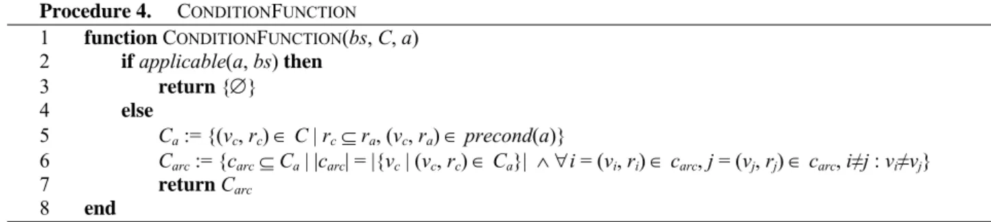
To generate the Extended Search Graph, we first introduce the EXTENDGRAPH procedure (Procedure 1), which creates nodes and arcs for the Extended Search Graph. Second, we present the CONDITIONS procedure (Procedure 2), which builds a set of conditions serving as the basis for constructing the branches in a given belief state. In this context, the PARTITION procedure (Procedure 3) is required to create disjoint partitions of the restrictions of belief state tuples. This procedure is provided in a third step. Finally, we introduce the CONDITIONFUNCTION procedure (Procedure 4), which builds the sets of conditions required to branch the Search Graph and label its arcs. How these parts of the algorithm work and how they interact with one another to construct the Extended Search Graph is described in the following and illustrated by our running example.
The EXTENDGRAPH procedure (Procedure 1) receives Search Graph SG and node bs. Clearly, the procedure is invoked for a belief state bs iff there are partly applicable actions in bs and an exclusive choice must be constructed accordingly. In a first step, by means of the CONDITIONS procedure, set C is built and contains the conditions required to construct the branches in node bs. Because these conditions depend on the preconditions of all partly applicable actions in bs and to avoid redundant calculations within the CONDITIONFUNCTION
procedure, which must be executed for each partly applicable action in bs thereafter, we decided to conduct this step beforehand. For belief state bs1 in our running example, the CONDITIONS procedure builds the set of conditions C := {(orderAmount, (0; 100) (100,000; 250,000]), (orderAmount, [100; 3,000)), (orderAmount, [3,000; 5,000]), (orderAmount, (5,000; 100,000]), (orderState, {valid}), (orderState, {invalid})} (details on how this set is built are provided in the CONDITIONS procedure).
For every action that is partly applicable in belief state bs, a set of sets of conditions Carc is built by executing
the CONDITIONFUNCTION procedure. For the action check competencies and belief state bs1 in our running example, the CONDITIONFUNCTION procedure returns the set of sets of conditions Carc := {{(orderAmount, [100; 3,000)), (orderState, {valid})}, {(orderAmount, [3,000; 5,000]), (orderState, {valid})}} (details on how this set is built are provided introducing the CONDITIONFUNCTION procedure).
In a next step, based on the set Carc, it is possible to construct the nodes and arcs that must be added to Search Graph SG to account for partly applicable action a in belief state bs (lines 5 to 9). Here, for each element carc of Carc, a new node representing new belief state bs’ (which can be reached by applying the action a in belief state bs) is built by applying the transition function cd(bs, carc, a) (Definition 16) and added to the set of nodes Nodes. Furthermore, new arcs bs, {precond(a), carc}, a and a, effects(a), bs’ are created between bs, a, and bs’ and added to the set of arcs Arcs. The outgoing arc of bs is thereby labeled with both the preconditions of action a and the corresponding set of conditions carc. For the action check competencies and belief state bs1, this results in the two nodes bs2,1 and bs2,2 (Figure 2) and the corresponding arcs (in Figure 2, we omitted depicting preconditions precond(a) and effects effects(a)).
Having added the nodes and arcs for all partly applicable actions in a Ap_a(bs), we finally add the arc
bs, else, termination to the Search Graph. This is because belief state bs might involve world states in which no action can be applied. In our running example, this condition is the case if belief state variable orderState equals invalid, for example.
Procedure 1. EXTENDGRAPH
1 procedure EXTENDGRAPH(bs, SG) 2 C := CONDITIONS(bs, SG) 3 forall a Ap_a(bs)
4 Carc := CONDITIONFUNCTION(bs, C, a) 5 forall carc Carc
6 bs’ := γcd(bs, carc, a) 7 Nodes := Nodes {bs’}
8 Arcs := Arcs {bs, {precond(a), carc}, a, a, effects(a), bs’}
9 endfor 10 endfor
11 Arcs := Arcs bs, else, termination
12 end
Within the EXTENDGRAPH procedure, the CONDITIONS procedure (Procedure 2) must be executed to derive the set of conditions C, which serves as a basis for constructing the branches of the Extended Search Graph in belief state bs. To this end, we initialize C with an empty set (line 2). Furthermore, we derive set bspre which contains all belief state tuples (vbs, rbs) of bs for which belief state variable vbs is in the precondition, but restriction rbs is not a subset of the corresponding restriction rpre for at least one action ap_a, which is partly
applicable in bs (line 3). In other words, for all belief state tuples (vbs, rbs) in bspre, there is at least one action which is partly applicable (i.e., this action cannot be applied in all possible world states of belief state bs concerning restriction rbs of belief state variable vbs). For belief state bs1 in our running example, considering the partly applicable actions check competencies and check extended competencies, set bspre equals {(orderAmount, (0; 250,000]), (orderState, {valid, invalid})}.
Then, for each belief state tuple (vbs, rbs) of bspre, we build the set of conditions Cpart to account for the preconditions of all partly applicable actions in bs and add them to the set of conditions C (lines 4 to 9). To do this, we first build set R consisting of all restrictions rpre that refer to belief state variable vbs and are part of the preconditions of the partly applicable actions in belief state bs. Next, to partition restriction rbs of belief state variable vbs in pairwise disjoint sets considering the restrictions rpre R, we execute the PARTITION procedure with rbs and R. Thus, restriction rbs of belief state variable vbs is partitioned such that it is clearly defined for each pairwise disjoint set and each action which is partly applicable in bs, whether the action can be applied in all possible world states or no world state at all with respect to this belief state variable vbs. The PARTITION
procedure is described in detail later on in this subsection. When deriving the set Partition for the belief state tuple (orderAmount, (0; 250,000]), for example, the PARTITION procedure is executed with rbs := (0; 250,000]
and R := {[100; 5,000], [3,000; 100,000]}. Here, the set of restrictions R consists of the restrictions concerning belief state variable orderAmount, which are part of the preconditions of the partly applicable actions check competencies and check extended competencies. In our example, executing the PARTITION procedure with rbs
and R, results in the set Partition := {(0; 100) (100,000; 250,000], [100; 3,000), [3,000; 5,000], (5,000; 100,000]}. In the next step, based on set Partition, set Cpart is built, which contains the set of belief state tuples (vbs, rp) containing a restriction rp that is an element of set Partition. For the belief state tuple (orderAmount, (0; 250,000]), set Cpart equals {(orderAmount, (0; 100) (100,000; 250,000]), (orderAmount, [100; 3,000)), (orderAmount, [3,000; 5,000]), (orderAmount, (5,000; 100,000])}.
Finally, having executed lines 4 to 9 for each belief state tuple of bspre and having extended the set of conditions C, the resulting set C is returned by the CONDITIONS procedure. In our running example for bs1 the set {(orderAmount, (0; 100) (100,000; 250,000]), (orderAmount, [100; 3,000)), (orderAmount, [3,000; 5,000]), (orderAmount, (5,000; 100,000]), (orderState, {valid}), (orderState, {invalid})} is returned.