Protein Stability in Mixed Solvents:
From Transfer Thermodynamics to the Denaturation by Urea
and Back
Dissertation
zur Erlangung des Doktorgrades der Naturwissenschaften (Dr. rer. nat.) der Fakultät für Chemie und Pharmazie
der Universität Regensburg
vorgelegt von Beate Moeser
aus Saarbrücken
im Jahr 2015
Die Arbeit wurde angeleitet von: Prof. Dr. Dominik Horinek
Prüfungsausschuss: Vorsitzender: Prof. Dr. Hubert Motschmann 1. Gutachter: Prof. Dr. Dominik Horinek 2. Gutachter: Prof. Dr. Pavel Jungwirth weiterer Prüfer: Prof. Dr. Christine Ziegler
Abstract
The conformational equilibrium between folded and unfolded protein structures is sensitive to the presence of cosolvents in the surrounding solution, and several small organic molecules are known to modulate the functioning of proteins in cells by shifting the equilibrium toward folded (stabilizers) or unfolded states (denaturants). The molecular mechanisms behind these effects are not yet fully understood and are a matter of intense research. In the past, successful models have been devised which predict the effects of cosolvents on proteins on the basis of their effects on small model compounds.
E. g., in the popular transfer model (TM) the latter are quantified by the free energies of the transfer (TFEs) of the model compounds between water and cosolvent solutions.
In this thesis, we examine and discuss the interpretation and measurement of TFEs.
Moreover, we deal with the application of TFE-based bottom-up approaches in the study of the denaturing mechanism of urea—the probably most studied and nonetheless most controversially discussed cosolvent. The highlights of this work are:
• We present a detailed and comprehensible explanation for the role of the con- centration scale in the definition of TFEs and show that only the TFE that is defined in the molarity scale can be interpreted directly in terms of favorable or unfavorable solute-solvent interactions.
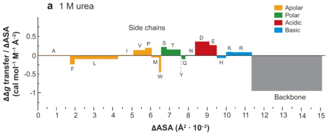
• We uncover an inconsistency and a compensating error in the nowadays established implementation of the TM. After their revision, the TM predicts that both the protein backbone and the side chains play a role in denaturation by urea. This is in line with many recent studies and thus paves the way toward a unified understanding of urea’s denaturing mechanism. Previous applications of the TM predicted a contrasting mode of action and this discrepancy was considered a major concern.
• We present a molecular dynamics study which provides further insight into urea’s denaturing mechanism. It suggests that protein denaturation by urea is the resultant of a complex and subtle interplay of various types of interactions between all solution components, being the protein, urea, and water.
• We propose a new measuring method for the determination of TFEs for transfers between pure and mixed solvents and point out that it is necessary to reassess the accuracies of currently employed measuring approaches. First steps into that direction suggest that some currently used measuring methods might not be as accurate as presumed so far.
Contents
1 Introduction and Outline 1
2 Chemical Potentials and Derived Quantities in Different Concentration
Scales 5
2.1 Introduction and Outline . . . 5
2.2 Concentration Scales . . . 6
2.3 Representations of the Chemical Potential . . . 7
2.3.1 Representation in the Framework of Statistical Thermodynamics 7 2.3.2 Representations in Terms of Standard Chemical Potentials and Activity Coefficients . . . 9
2.3.2.1 Dilute Solution as Reference . . . 9
2.3.2.2 Different Definitions of the Dilute Reference State in Ternary Solutions . . . 15
2.3.2.3 Pure Substance as Reference . . . 17
2.4 Interpretation of Dilute-Reference Activity Coefficients . . . 18
3 The Concept of Transfer Free Energies 25 3.1 Introduction and Outline . . . 25
3.2 The Role of the Concentration Scale in the Definition of TFEs . . . 26
3.2.1 Outline of the Problem . . . 26
3.2.2 Different Transfer Processes at Infinite Dilution . . . 27
3.2.3 Conversion between Standard TFEs . . . 29
3.2.4 Interpretation of Standard TFEs . . . 31
3.2.5 Implications for Related Quantities . . . 34
3.2.6 Differences in TFEs of Different Solutes . . . 35
3.2.7 Advantageous Concentration Scales in Experiments . . . 35
3.2.8 Concluding Remarks . . . 36
3.3 Measurement of TFEs . . . 36
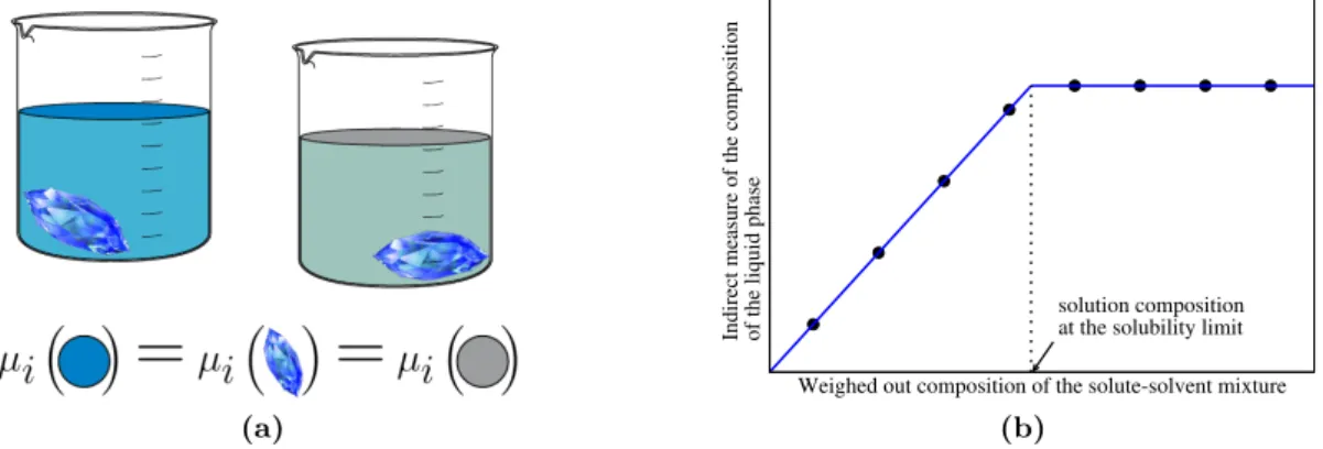
3.3.1 Solubility Measurements . . . 37
3.3.2 Vapor-Pressure Measurements . . . 39
3.4 Determination of TFEs in Molecular Dynamics Simulations . . . 40
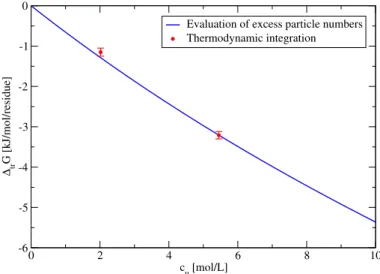
3.4.1 Evaluation of Excess Particle Numbers . . . 40
3.4.2 Thermodynamic Integration . . . 43
3.4.3 Consistency of the Two Methods . . . 44
3.A Appendix . . . 46
3.A.1 Supplements to Section 3.2: TFEs at Constant Finite Concentrations 46 3.A.2 Supplements to Section 3.3: Measurement of Activity Coefficients 47 3.A.2.1 Measurement of the Solvent Activity . . . 47
3.A.2.2 Determination of the Activity Coefficients of the Solutes from the Activity of the Solvent . . . 49
3.A.3 Supplements to Section 3.4 . . . 53
3.A.3.1 A Short Introduction into Molecular Dynamics Simulations 53 3.A.3.2 Simulation Details . . . 53
4 The Transfer Model for Urea Denaturation Revisited 57 4.1 Overview . . . 57
4.2 Background Information . . . 58
4.2.1 The Notion of Urea’s Denaturing Mechanism Over Time . . . 58
4.2.2 The Transfer Model . . . 59
4.2.2.1 First Formulation by Tanford . . . 59
4.2.2.2 Nowadays Established Implementation by Auton and Bolen . . . 61
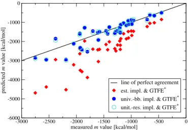
4.2.2.3 Results Obtained by the Established TM . . . 64
4.2.2.4 Perception of the TM: A Story of Success and Criticism 66 4.3 Two Revisions of the Established TM . . . 67
4.3.1 Revision of the Implementation of the ASA-Scaled Additivity . . 67
4.3.1.1 Motivation . . . 67
4.3.1.2 Validation of the ASA-Scaled Additivity Assumption by Molecular Dynamics Simulations . . . 70
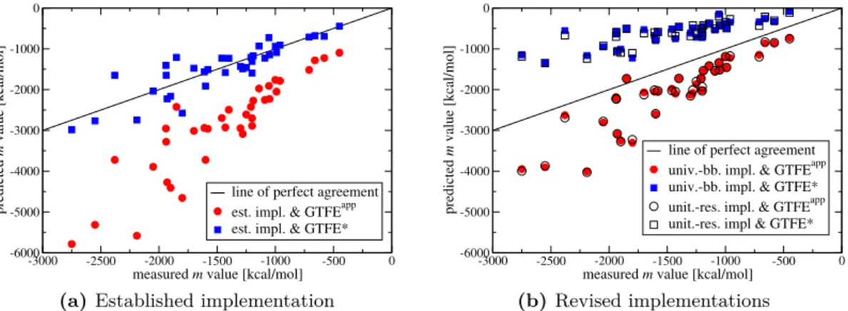
4.3.1.3 Effect of the Revision on m-Value Predictions . . . 76
4.3.2 Revision of the Side-Chain TFEs . . . 77
4.3.2.1 The Miscalculation in the GTFE* Set of Side-Chain TFEs . . . 77
4.3.2.2 Effect of the Revision on m-Value Predictions . . . 81
4.4 Backbone and Side-Chain Contributions to Denaturation . . . 82
4.5 Discussion and Outlook . . . 85
4.A Appendix . . . 88
4.A.1 Materials and Methods . . . 88
4.A.1.1 Molecular Dynamics Simulations . . . 88
4.A.1.2 m-Value Predictions for Proteins . . . . 92
4.A.2 Supplements to Section 4.3.1.2 . . . 95
5 Insights into Urea-Protein Interactions from Molecular Dynamics 101 5.1 Introduction . . . 101
5.2 The Macroscopic Perspective . . . 102
5.3 Toward a Microscopic Perspective . . . 104
5.3.1 Denaturation by Accumulation at the Peptide Surface . . . 104
5.3.2 Driving Forces for the Accumulation of Urea at the Peptide . . . 105
5.3.2.1 Simulation Setup . . . 105
Contents
5.3.2.2 Gibbs Free Energy of Adsorption . . . 106
5.3.2.3 Energy of Adsorption . . . 108
5.3.2.4 Entropy of Adsorption . . . 113
5.3.3 Orientation and Position of Urea at the Peptide Surface . . . 114
5.3.3.1 Definition of Angles . . . 115
5.3.3.2 Inclination of the Urea Plane . . . 117
5.3.3.3 Exact Orientation of Urea at the Peptide Surfaces . . . 118
5.4 Summary and Outlook . . . 130
5.A Appendix . . . 132
5.A.1 Calculation of the Free-Energy Profiles . . . 132
5.A.2 Calculation of the Differences in Pairwise Interaction Energies . 133 5.A.3 Analysis of the Position and Orientation of Urea . . . 135
6 A New Measuring Method for Transfer Free Energies 139 6.1 Overview . . . 139
6.2 Motivation . . . 140
6.3 The Proposed Measuring Method . . . 141
6.3.1 Idea of the Method . . . 141
6.3.2 Generic Measuring Instruction . . . 145
6.3.3 Proof of Concept . . . 147
6.4 Estimation and Optimization of the Accuracy . . . 148
6.4.1 Accuracy of Measurements of Osmotic Coefficients . . . 148
6.4.2 The Concept of Monte Carlo Error Estimations . . . 149
6.4.3 The “Proof of Concept” under More Realistic Conditions . . . . 150
6.4.4 Reduction of the Statistical Uncertainty . . . 151
6.4.5 Further Considerations Regarding the Accuracy . . . 154
6.5 A Variant of the Proposed Method . . . 158
6.5.1 Introduction and Derivation . . . 158
6.5.2 Theoretical Considerations . . . 160
6.6 Comparison to Established Measuring Methods . . . 162
6.6.1 VPO Measurements According to Record and Co-Workers . . . . 162
6.6.2 Other Measuring Methods . . . 166
6.7 Discussion and Outlook . . . 167
6.A Appendix . . . 169
6.A.1 Hypotheses Concerning the Conditions under which Apparent TFEs are Good Approximations to STFEs . . . 169
6.A.2 Supplements to Section 6.4 . . . 173
6.A.3 Feasibility of the Variant . . . 177
7 Discussion and Outlook 181
Bibliography 183
Acronyms and Symbols
Acronyms
ASA solvent accessible surface area, page 60 GTFE group transfer free energy, page 62 GTFEapp apparent group TFEs, page 62 GTFE* so far established GTFEs, page 62
GTFE+ correct recalculation of the GTFE* values, page 79 KBI Kirkwood-Buff integral, page 20
MD molecular dynamics, page 40
PME particle-mesh Ewald, page 134
rms root mean square, page 73
SDF spatial distribution function, page 122 STFE standard transfer free energy, page 29 TFE transfer free energy, page 25
TM transfer model, page 57
VPO vapor-pressure osmometry, page 48
Frequently Used Symbols
a1 activity of the solvent,γ1,x∗ ·x1, page 47
c, ρ molarity, page 6
d mass density, page 13
∆ (m2+m3)ϕ23−m2ϕ2−m3ϕ3, page 141
∆trG0i,ξ(a→b) ξ-scale STFE of a solute ‘i’ for transfers between ‘a’ and ‘b’1, page 26
∆unfG Gibbs free energy of unfolding of a protein, page 2
Γi excess of particles of type ‘i’ in the vicinity of a solute, page 41 gij(r) pair correlation function, radial distribution function, page 20 Gij Kirkwood-Buff integral, page 20
Kunf equilibrium constant of the unfolding reaction of a protein, page 59 ξ, θ variables which stand for any concentration scale, page 9
Λ thermal de Broglie wavelength, page 7
mˆ molality, page 6
m value a measure for the strength of a cosolvent effect on a protein, page 64
m aquamolality, page 6
M molar mass, page 13
µ23 chemical potential derivative, page 34 µ?i pseudo chemical potential, page 8
µ0i,ξ, γi,ξ0 dilute-reference standard chemical potential and activity coefficient of the solute ‘i’ in the concentration scale ξ, page 9
µ0,ξi,ξk, γi,ξ0,ξk as above, but defined in a mixed solvent with cosolvent concentration
‘ξk’1, page 15
µ00i,ξ, γi,ξ00 as above, but defined in a mixed solvent with variable cosolvent concentration, page 16
µ∗i, γi,x∗ standard chemical potential and activity coefficient of the solute ‘i’
with the pure substance as reference, page 17 ϕ osmotic coefficient, page 50
q internal partition function, page 7
V molar volume, page 12
W (i|s) coupling work of the solute ‘i’ to the solution ‘s’, page 8
x mole fraction, page 6
Indices Referring to Solution Components
1 (principal) solvent
2 solute
Acronyms and Symbols
3 cosolvent
Indices Referring to Proteinogenic Building Blocks
aa type of amino acid residue
bb backbone
sc side chain
Acronyms for Amino Acid Types
Ala, A alanine
Arg, R arginine
Asn, N asparagine
Asp, D aspartic acid
Cys, C cysteine
Gln, Q glutamine
Glu, E glutamic acid
Gly, G glycine
His, H histidine
Ile, I isoleucine
Leu, L leucine
Lys, K lysine
Met, M methionine
Phe, F phenylalanine
Pro, P proline
Ser, S serine
Thr, T threonine
Trp, W tryptophan
Tyr, Y tyrosine
Val, V valine
1Some of the sub- or superscripts are sometimes omitted when their meaning is clear from the context.
Chapter 1
Introduction and Outline
Proteins are biological macromolecules that play decisive roles in almost all biological processes: they catalyze reactions, transmit signals, transport molecules, maintain cell shape, control cell growth, and much more. They are the workhorses of the cell. Proteins are heteropolymers of 20 different amino acid subunits, and—depending on the primary sequence of the amino acid residues—they typically attain a specific three-dimensional structure which is essential for their function.
This so-called native or folded structure is only marginally stable and, thus, in a natural environment functional folded proteins always coexist with a small population of inoperative proteins in unfolded conformations. The conformational equilibrium between the different protein structures is highly sensitive to changes in external conditions, as e. g. temperature and pressure, and to the composition of the surrounding solution. In the current thesis, we deal with the latter and study the influence of cosolvents on protein stability. With the term “cosolvent” we here generally refer to solvent components other than water [39] and specifically mean small organic molecules that typically are present in biological cells, e. g. as metabolites, osmoregulators, or messenger substances.
These molecules (or subclasses of them) are sometimes also called cosolutes or osmolytes [147, 185]—due to their role in the osmotic homeostasis. Some cosolvents are denaturants and reversibly shift the conformational equilibrium of protein structures toward unfolded states. Others, so-called stabilizers, shift it toward the folded state. There is evidence that the effects of a range of cosolvents on protein folding equilibria are additive and that stabilizers are used in cells to antagonize the impact of denaturants [154, 185].
By the same token, some cosolvents can counteract changes in protein stability that are due to temperature and pressure changes [89, 186]. Interestingly, experiments suggest that too high concentrations of stabilizing cosolvents can be detrimental for organisms [185], which indicates that deviations in either direction from the natural conformational equilibrium between protein structures can be harmful [154, 185]. Or, as Somero phrased it, it seems to be vital to maintain the “correct balance between structural stability and lability” [154]. This might also explain why organisms that face high osmotic stresses typically use mixtures of stabilizers and denaturants for osmoregulation. Examples are marine cartilaginous fish that osmoconform to their salt
water surroundings by accumulation of stabilizing methylamines and the denaturant urea.
In the last decades, a massive amount of studies aimed at elucidating the molecular mechanisms underlying the cosolvent effects on proteins. Though, despite much progress, there are still many open questions and a conclusive understanding of cosolvent effects is yet to come. This might possibly be due to the fact that the molecular interactions between cosolvents, proteins, and other solution components are non-covalent and small in magnitude, which poses a challenge for their measurement as well as for their accurate modeling in computer simulations [39, 166, 142]. This is aggravated by the fact that the difference in free energy between the folded protein structure and its unfolded structure,
∆unfG, is small in magnitude as well: it is comparable to the energy of a single hydrogen bond [136].
The list of motivations underlying the current research on cosolvent effects on proteins is long: On the one hand it is expected that a better understanding of cosolvent effects on protein stability promotes a deeper insight into the longstanding protein folding problem [27, 136], which fascinates and puzzles researchers since the publication of the first protein structures and the works of Anfinsen [2, 65] and Levinthal [97] in the 1960s. Moreover, one hopes to achieve a better understanding of diseases which involve the misfolding of proteins; and one pursues the distant goal of treating them by administration of protein stabilizers [33, 162]. Preliminary successes in this respect have already been reported by experiments with cell cultures, which suggest that the protein stabilizers glycerol and trimethylamine N-oxide can correct folding defects of mutated proteins which are related to cystic fibrosis, tumor growth, or nephrogenic diabetes insipidus [32, 33, 162]. Cosolvents are also of high practical relevance in biotechnological processes and in the development of biopharmaceutical formulations [36, 148], where scientists often have to cope with protein misfolding, aggregation, and denaturation. In these areas, cosolvents are successfully employed on a trial-and-error basis nowadays—e. g. during refolding from inclusion bodies [3] or in the formulation of protein-based vaccines [29]. Yet, a thorough understanding of cosolvent effects on a molecular level would facilitate predictions and enable the possibility for the design of specific additives for specific applications [36]. This would render large-scale screening experiments superfluous.
Among all organic cosolvents, the protein denaturant urea was so far probably studied longest and most intensely so that it well can be termed to be the “drosophila” of cosolvent studies. As a metabolic product of protein and amino acid degradation, urea is a ubiquitous cosolvent in mammals and amphibians. Its denaturing effect on proteins was already discovered around 1900 [156] and since then urea is widely used as a denaturing agent in biochemical laboratories. Yet, even today, the molecular mechanism of protein denaturation by urea is a matter of controversial scientific debate.
In the present thesis, we contribute to this debate and focus on the effect of urea when analyzing cosolvent effects on proteins. Throughout the work, we will typically use urea as a representative for cosolvents. Yet, several of our studies concern very fundamental aspects of the measurement and interpretation of cosolvent effects on solutes so that their results are equally applicable to all kinds of cosolvents.
In the recent years, a broad variety of methods was applied in the research on the effects of urea and other cosolvents on proteins. On the side of theoretical approaches, molecular dynamics simulations proved exceptionally valuable (see ref. [39] and references therein) as they give direct access to thermodynamic properties of solutions and even provide detailed information on intermolecular interactions. On the experimental side, some important insights were obtained by spectroscopic techniques [53, 68, 72, 82, 104, 141], however, more popular and among the most successful strategies were bottom-up approaches which try to understand the cosolvent effects on proteins with the help of experiments on small model molecules [10, 11, 94, 129, 164]. The cosolvent effects on those model molecules, which resemble the proteinogenic building blocks, are quantified by measurements of thermodynamic parameters. Different models have been devised which allow to predict cosolvent effects on protein folding equilibria on the basis of such data [8, 129, 164]. Given that the assumptions underlying these predictions are correct, these models provide an explanation of cosolvent effects on protein stability on the level of individual building blocks. The most prominent of these bottom-up approaches is probably the transfer model, which was proposed by Tanford in the 1960s [164] and rendered implementable by Auton and Bolen [7, 8, 9, 101] in the last 20 years. In this model, the cosolvent effects on the small model compounds are quantified by the free energies of transferring them from water to a cosolvent solution.
In the thesis at hand, we focus on the transfer model and related bottom-up approaches and examine them from various angles by means of theoretical considerations and simulation studies: On the one hand, we directly deal with the results that the transfer model yields for the denaturing mechanism of the protein denaturant urea—and provide an explanation for longstanding mismatches between the predictions of the transfer model and the results of other studies on urea’s mode of action. On the other hand, we take a very basic point of view on transfer approaches and concern ourselves with theoretical and practical aspects of the interpretation and measurement of transfer free energies. In the following, we provide a brief overview over the various studies that we present in this thesis and outline the content of the upcoming chapters.
Inchapter 2, we lay the theoretical groundwork for our studies and discuss several representations of the chemical potential of components in mixed solvents. We especially focus on the role of the choice of concentration scale and reference state in the definition of standard chemical potentials and activity coefficients. This topic, which is rarely addressed in textbooks or the literature, will be of high relevance throughout the thesis.
Moreover, we discuss a statistical-thermodynamical representation of the chemical potential, which we later on recurrently employ to comprehensibly interpret abstract thermodynamical expressions.
Subsequently, inchapter 3, we introduce the concept of transfer free energies which are used in the transfer model to quantify in how far a proteinogenic building block favors (or disfavors) a cosolvent solution over pure water. We explain in much detail how transfer free energies are defined and which role the concentration scale plays in their definition. This point, which is controversially discussed in the literature, is very crucial because if the concentration scale is not properly accounted for in the interpretation of measured transfer free energies, severe misinterpretations of the solvent preferences can arise. We will explain comprehensibly why only the transfer free energy that is
defined in the molarity concentration scale directly yields insights into solute-solvent interaction free energies. This finding is of high relevance for all applications in which transfer free energies are employed to quantify solvent preferences of solutes.
Moreover, we explain in chapter 3 how transfer free energies commonly are measured and how they can be determined in molecular dynamics simulations. A basic knowledge thereof will be needed to understand the studies in the subsequent chapters.
Chapter 4deals with the application of the transfer model to the problem of protein denaturation by urea. In that context, the transfer model recently was often criticized because the denaturing mechanism that it so far predicted was at odds with results of other studies: while a wealth of recent studies ascribes protein denaturation by urea to favorable interactions between urea and both the backbone and the side-chain groups of proteins, the transfer model so far attributed it exclusively to urea-backbone interactions. In chapter 4, we will provide an explanation for this mismatch: we uncover an inconsistency and a compensating error in the nowadays established implementation of the transfer model and show that their revision brings the transfer model in line with a view in which both the backbone and the side chains contribute to protein denaturation by urea. This is a very important step toward a unified understanding of urea’s denaturing mechanism.
Afterward, in chapter 5, we dwell on the subject and elaborate more on urea’s denaturing mode of action: we employ molecular dynamics simulations to study the interactions between urea and different kinds of peptide surfaces. We quantify the average contributions of different types of molecular forces to the urea-peptide interaction and characterize these interactions on a sub-thermodynamical level by analyzing prominent orientations and positions of urea at the chemically heterogeneous peptide surfaces.
The molecular dynamics study reveals a complex interplay between the peptides, urea, and water so that it seems safe to rule out that protein denaturation by urea can be explained by simple models which only account for one type of urea-protein interaction (and disregard water).
Eventually, in chapter 6, we turn back to transfer free energies and propose a new measuring method for them. This method was not yet applied in practice, but in theory it is exact and Monte Carlo error estimations are very promising. The validation of the newly proposed method—and of variants thereof—by Monte Carlo error simulations does not only show their potentialities and limitations, but also reveals that it is important to reassess the accuracy of currently used measuring methods for transfer free energies. This is, among other things, because most of the measuring approaches that are typically used nowadays are based on approximations whose influences on the measuring result were not yet characterized. This also concerns the approaches used in the transfer model and related models. To make a start, we analyze one established measuring method and demonstrate that it is markedly less accurate than presumed so far. We hope that our propositions and analyses presented in chapter 6 promote the development of new efficient and accurate measuring techniques for transfer free energies.
Chapter 7 concludes the thesis with a final discussion and an outlook, in which we point to the relevance of our results in the bigger picture.
Chapter 2
Chemical Potentials and Derived Quantities in Different Concentration Scales
2.1 Introduction and Outline
In the present thesis, we study in how far the solvent environment influences the stability of proteins. Probably the most prominent model for the description thereof is the transfer model, which will be examined (and revised) in chapter 4. In the framework of the transfer model, solvent effects on protein stabilities are traced back to the solvent preferences of the different types of proteinogenic building blocks. These solvent preferences are quantified by transfer free energies, which we will introduce in detail in chapter 3. In that context, we will show that there are disagreements about the proper definition of these transfer free energies in the recent literature, which have a tremendous impact on their interpretation. These confusions, which we will settle in chapter 3, concern the role of the concentration scale used in the definition of the transfer free energies. In large parts, these confusions can be traced back to the fact that the underlying quantity, the chemical potential, typically is split up into a concentration-dependent and a concentration-independent term. This split-up into two terms introduces two auxiliary quantities (a standard chemical potential and an activity coefficient) that depend non-trivially on the choice of concentration scale and the choice of reference state in their definition. In the chapter at hand, we lay the groundwork for the upcoming chapters and elaborate on the concentration-scale and reference-state dependence of standard chemical potentials and activity coefficients—a fundamental topic which only rarely is taken note of.
In the following, we will introduce the most common conventions for the definition of standard chemical potentials and activity coefficients. We will point out the differences between them and will derive universally valid equations for the conversion of standard chemical potentials and activity coefficients between concentration scales and reference states. These conversion equations will be needed in the upcoming chapters. We will
introduce the different notations in a rather formal way. That is because we consider it very important to properly define them since the differences are subtle and decisive at the same time. In chapter 4, we will give a striking example in which a neglect of these subtleties in the conversion of activity coefficients between concentration scales had far-reaching consequences: we will argue that this neglect—among other things—is accountable for a presumably incorrect view of protein denaturation by urea that was promoted by recent implementations of the transfer model.
All here introduced definitions of standard chemical potentials and activity coefficients will be used at some point in this thesis. Thus, as a side effect, the present chapter also serves to introduce and set the notation used in the thesis. Yet, the chapter does not only deal with formal definitions and the establishing of notations: special emphasis will be placed on the effect that the concentration scale and the reference state have on the interpretation of the standard chemical potential and the activity coefficient. To address the latter, we first present a representation of the chemical potential in the framework of statistical thermodynamics. By comparison with this statistical-thermodynamical expression it is possible to assign interpretations to the various standard chemical potentials and activity coefficients. Furthermore, at the end of the chapter, we will devote a section to the question how activity coefficients can be interpreted.
As a start, we first define the different concentration scales in the following section.
2.2 Concentration Scales
The composition of a solution can be specified in numerous conceptually different ways, which are referred to as “concentration scales”. The most commonly used concentration scales are
• molarityc (orρ): molecules per volume of the solution,
• mole fraction x: molecules per total number of molecules,
• molality ˆm: molecules per mass of solvent (which in ternary solutions is the mixture of the principal solvent and the cosolvent),
• (aqua-)molalitym: molecules per mass of water (resp. more generally the principal solvent).
In binary solutions of a solute and a solvent, the aquamolalitymand the molality ˆmare identical and usually simply called molality m. In ternary solutions, the term molality (and the symbolm) is ambiguously used. Sometimes it refers to “moles per kg of water”
and sometimes to “moles per kg of mixed solvent”. To avoid misunderstandings, we here use distinct symbols for the two molalities.
Other concentration scales, which are less frequently used in solution thermodynamics and only mentioned here for the sake of completeness, are molonity ˜m (molecules per mass of the solution) and mass fraction w(mass per mass of the solution).
It is important to note that the choice of concentration scale is more than simply a choice of units: the above list demonstrates that the scales define different quantities.
2.3 Representations of the Chemical Potential
In fact, the concentration in each scale can be expressed in various units (e. g. molarity in 1/m3 or in mol/L) and concentrations given in clearly different concentration scales can have the same units (e. g., x and worm, ˆm, and ˜m).
2.3 Representations of the Chemical Potential
Before we turn to representations of the chemical potential in terms of a standard chemical potential and an activity coefficient, we describe in the following section how the chemical potential can be expressed in the framework of statistical thermodynamics.
The statistical-thermodynamical expression motivates why the chemical potential is typically split-up into two summands. Moreover, this expression will be frequently used in this thesis to interpret quantities that can be derived from chemical potentials (as e. g. activity coefficients and transfer free energies).
2.3.1 Representation in the Framework of Statistical Thermodynamics For the statistical-thermodynamical description, we consider a solution of Ni solute particles and Nj solvent particles. In principle, the solvent could be a mixture of different types of molecules (e. g., a solvent and a cosolvent). For the points made here, it is, however, not necessary to distinguish between different solvent components so that we use the indexj to refer to the solvent in general.
At constant pressure and constant temperature, the chemical potential µi of the solute in the considered solution is defined by
µi = ∂G
∂Ni
p,T ,Nj
. (2.1)
It describes the change in Gibbs free energy upon the addition of a single solute molecule to the solution. In ref. [18], Ben-Naim derived a statistical-thermodynamical expression forµithat is valid in the classical limit of statistical thermodynamics and thus applicable to liquid solutions at room temperature. It reads
µi=−kTln
exp
−∆Ui(R0) kT
0
+kTln ρiΛ3i qi
!
. (2.2)
ρi is the molarity (i. e. molecules per volume) of the solute ‘i’ in the solution, Λi is its thermal de Broglie wavelength, and qi the internal (i. e. rotational, vibrational, electronic, and nuclear) partition function of the solute (in the solution). ∆Ui(R0) is the change in system energy upon the addition of a solute molecule ‘i’ at a fixed position R0 to the solution at a specific configuration:
∆Ui(R0) =U(Ni+ 1, Nj)−U(Ni,Nj). (2.3) Here, (Ni, Nj) stands for a specific configuration of the molecules in the solution. The averagehi0 in Eq. (2.2) is over all possible configurations of the molecules in the solution except the one that was added. Ben-Naim sometimes calls the latter molecule “solvaton”
[18, 19] to distinguish it from the other solute molecules of type ‘i’ that already are in the solution.
The first term on the rhs of Eq. (2.2) is the average work to add a molecule of type ‘i’
to any fixed positionR0 in the solution consisting ofNi solute andNj solvent molecules.
It accounts for the Gibbs energy of interaction between the solvaton and its entire surroundings. From now on, we will abbreviate this coupling work of a molecule of type
‘i’ to a given solution ‘s’ by W(i|s). ‘s’ stands for the solution under consideration, which is a mixture of molecules of type ‘i’ and ‘j’ with a given composition. A solution in which the solute ‘i’ is infinitely dilute will be denoted by ‘s0’. Thus, W i|s0is the coupling work of a molecule of type ‘i’ to the pure solvent ‘j’. The second term on the rhs of Eq. (2.2) corresponds to the chemical potential of the solute ‘i’ that it had if the solution were an ideal gas.
While µidescribes the change in Gibbs free energy upon addition of a solute molecule to the solution, Ben-Naim also derived an expression for the change in Gibbs free energy of the system for the special hypothetical case that the solute is added to any fixed position in the system (with the constraint to stay there and to be distinguishable from the other solute molecules). This change in Gibbs free energy is given by
µ?i =−kTln
qi·
exp
−∆Ui(R0) kT
0
(2.4)
=W(i|s)−kTln (qi). (2.5)
Ben-Naim coined the term “pseudo chemical potential” for µ?i. A combination of Eqs. (2.2) and (2.4) yields
µi =µ?i +kTlnρiΛ3i. (2.6) This representation of the chemical potential suggests that one can envision the addition of a solute particle to a solution as a two-step process: In the first step, the solute is added to a fixed position in the solution. Thereby, the Gibbs free energy of the system changes by µ?i due to the additional interaction free energy W (i|s) and the additional degrees of freedomqi. In the second step, the constraint of a fixed position is released and the solvaton is allowed to blend in the rest of the solution. Thereby, it gains translational degrees of freedom which contributekTln Λ3i/Vto the Gibbs free energy. Moreover, releasing the constraint makes the solvaton indistinguishable from the rest of the solute molecules. This contributeskTln (Ni) to the Gibbs free energy of the system. The contribution of the second step is often called “liberation free energy”
[17, 18].
The above discussion shows that the chemical potential depends in several ways on the solute concentration ρi of the considered solution:
• explicitly (and trivially) through the liberation free energy,
• and implicitly through the dependence of the pseudo chemical potential (the coupling work and the internal partition function) on the solution composition.
2.3 Representations of the Chemical Potential
2.3.2 Representations in Terms of Standard Chemical Potentials and Activity Coefficients
We will now show how the different contributions toµi in Eq. (2.6) can be mapped onto representations of the chemical potential in terms of a standard chemical potential and an activity coefficient. In the following section, we first consider representations with a dilute-solution reference state, which are commonly used for the chemical potential of solutes in solutions and, thus, are also predominantly employed in the current thesis.
In a general form, these dilute-reference representations can be written as µi =µ0i,ξ+kTlnγi,ξ0 ·ξi with lim
ξi→0
γi,ξ0 = 1, (2.7) whereξi expresses the concentration of the solute in any concentration scale. µ0i,ξ is the standard chemical potential and γi,ξ0 the activity coefficient, which depends on the solute concentration. The superscript 0 denotes that the two quantities are defined for a dilute-solution reference state, and the subscript ξ indicates the concentration scale for which they are defined by Eq. (2.7). As the “natural concentration scale” in statistical thermodynamics is the molarity scale, we will first show that the representation in Eq. (2.7) is possible in the molarity scale. Afterward, we will demonstrate that the same functional form can also be used for other concentration scales. Due to the constraint that is set on the activity coefficient in Eq. (2.7), it is not trivial that this is generally possible. Subsequently, we derive equations for the conversion of the µ0i andγi0 between different concentration scales. These are often needed when one seeks to compare data published in different notations and they will be of relevance in chapters 3 and 4. In section 2.3.2.2, we will address different representations of chemical potentials in ternary solutions for which the definition of a dilute reference state is ambiguous. Later, in section 2.3.2.3, we will turn to representations of the chemical potential in which the chemical potential of the pure liquid substance is taken as the standard chemical potential. This representation is typically chosen for the solvent in a solution.
2.3.2.1 Dilute Solution as Reference
Let us now analyze what the above defined µ0i,ξ and γi,ξ0 stand for in the different concentration scales and how they are related to one another.
Molarity Scale
According to Eq. (2.7), the standard chemical potential µ0i,ρ in the molarity scale is defined by
µ0i,ρ= lim
ρi→0(µi−kTln (ρi)). (2.8) Evaluation of Eq. (2.8) with help of Eqs. (2.6) and (2.5) reveals
µ0i,ρ=µ?i s0+kTlnΛ3i (2.9)
=W i|s0−kTlnqi
s0+kTlnΛ3i. (2.10)
Thus, we see that the dilute-reference standard chemical potential in the molarity scale µ0i,ρ accounts for the coupling work of the solute to the pure solvent of the solution as well as for the internal partition function of the solute at infinite dilution in the solution.
Moreover, it incorporates parts of the translational partition functionqtrans,i=V /Λ3i of the solute in the solution, where we assume thatΛi is independent of the solution composition. The value of the standard chemical potentialµ0i,ρ does not correspond to the value of the chemical potential of the solute ‘i’ at a reference composition of the considered solution. Instead, a comparison of Eq. (2.9) to Eq. (2.6) reveals that µ0i,ρcan be understood as being the chemical potential of the solute at concentrationρi = 1 in a hypothetical solution in which the pseudo chemical potential µ?i does not depend on the solute concentration ρi (i. e., the Gibbs free energy of adding a particle to a fixed position in the hypothetical solution equals for all solute concentrations the Gibbs free energy of adding a particle to a fixed position in the pure solvent).
Insertion of Eq. (2.9) into Eq. (2.7) for the molarity scale (i. e., ξ=ρ) and comparison with Eq. (2.6) reveals that the termkTlnγi,ρ0 accounts for the difference of the pseudo chemical potential at the solute concentration ρi and the pseudo chemical potential at infinite dilution of the solute1:
kTlnγi,ρ0 =µ?i (s)−µ?is0. (2.11) Hence, kTlnγi,ρ0 describes to what extent a solution with solute concentration ρi
affects the solvaton differently than the pure solvent does. This term bridges the gap between the chemical potential of the above described hypothetical solution and the chemical potential of the real solution. A more detailed discussion of the interpretation of the activity coefficient will be given in section 2.4.
With Eqs. (2.9) and (2.11) we have shown that it is possible to express the chemical potential in terms of a standard chemical potential and an activity coefficient in the molarity scale. Before we turn to other concentration scales, we want to see how the molarity-scale standard chemical potential and activity coefficient are affected by the choice of units in which the molarity of the solute is expressed. Assume c expresses the molarity in different units thanρ (e. g.,c in mol/L and ρ in 1/m3) and the two are converted by a factorK (ρ=K·c, withK = 1000·NA in the example). Then, the calculation ofµ0i,c and γi,c0 (analogously to the calculation of µ0i,ρ and γi,ρ0 ) reveals
γi,c0 =γi,ρ0 , (2.12)
µ0i,c=µ0i,ρ+kTln (K). (2.13) Thus, the molarity-scale activity coefficient is independent of the units in which the molarity is expressed and the molarity-scale standard chemical potential depends on them. While the numerical value of µ0i,ρ equals the chemical potential in the above
1If we drop the assumption thatΛ3i is independent of the solution composition,kTln γi,ρ0
contains an additional termkTln Λ3i(s)/Λ3i s0
which quantifies the effect of the solution onΛi. Then, µ0i,ρdepends only onΛi s0, the thermal de Broglie wavelength of the solute at infinite dilution in the solvent.
2.3 Representations of the Chemical Potential
described hypothetical solution atρi= 1, the numerical value ofµ0i,cequals the chemical potential of the same hypothetical solution atci = 1, in which case there are a factor of K more indistinguishable particles in the solution than atρi = 1. From now on, we will use the letter cto refer to the molarity scale.
Other Concentration Scales
In the following, we derive expressions for the infinite-dilution standard chemical potential and the corresponding activity coefficient for all concentration scales ξ that fulfill the following four criteria:
1. The zero point is the same as in molarity scale ξ(c= 0) = 0.
2. ξ(c) is strictly monotonic.
3. ξ(c) is continuous.
4. The derivative ∂ξ/∂c atξ= 0 is not zero.
For such concentration scales, the zeroth-order term of the Taylor expansion ξ(c) in the point c= 0 is zero and the first-order term is non-zero:
ξ(c) = ∂ξ
∂c c=0
·c+Oc2. (2.14)
All concentration scales listed in section 2.2 fulfill these criteria so thatξ may stand here for any of them. To find expressions for µ0i,ξ andγi,ξ0 with which the chemical potential µi can be written in the form of Eq. (2.7), we require the following relation
µ0i,ξ+kTln (ξi) +kTlnγi,ξ0 =µi =µ0i,c+kTln (ci) +kTlnγi,c0 (2.15) for allsolution compositions. Evaluation of Eq. (2.15) in the limit of infinite dilution allows to find an expression for the ξ-scale standard chemical potential
µ0i,ξ =µ0i,c+kTln
climi→0
ci ξi
+kTln lim
ci→0
γi,c0 γi,ξ0
!!
. (2.16)
By definition, γi,ξ0 and γi,c0 are both unity in the considered limit so that the third term on the rhs of Eq. (2.16) vanishes. The second term on the rhs of Eq. (2.16) exists according to Eq. (2.14) and equals ∂ci/∂ξi|c
i=0. Hence,µ0i,ξ can be identified as µ0i,ξ =µ0i,c+kTln
climi→0
ci ξi
. (2.17)
Inserting this back into Eq. (2.15) yields an expression for the ξ-scale activity coefficient γi,ξ0 = lim
ci→0
ξi ci
·ci
ξi ·γi,c0 . (2.18)
Thus, it is possible to express the chemical potential for all concentration scales ξ that fulfill the above criteria in terms of a standard chemical potential and an activity
coefficient that goes to 1 in the limit ξ → 0. From the above equations, we see that forcing the expressionµi(ξi) to have the same functional form asµi(ci), i. e. the form of Eq. (2.7), for all concentration scales ξ implies that all concentration-dependent terms of the concentration-scale conversionci ⇒ξi must be included in the activity coefficient γ0i,ξ.
Conversions of Dilute-Reference Standard Chemical Potentials and Activity Coefficients between Concentration Scales
Eqs. (2.17)–(2.18) relate the standard chemical potentialµ0i,ξ and the activity coefficient γ0i,ξ of any concentration scale ξ to the respective quantitiesµ0i,c andγi,c0 of the molarity scale. Here, we want to generalize these relations to any two concentration scales, ξ and θ, to obtain general conversion equations between infinite-dilution standard chemical potentials and activity coefficients:
We require that both concentration scales ξ andθfulfill the four criteria listed above.
If this is given, the criteria also hold between them. Thus, having shown thatµ0i,ξ and γ0i,ξ exist for the scaleξ, we can repeat the derivations (2.15)–(2.18) withθandξinstead of ξ and c, and get the general conversion equations:
µ0i,θ =µ0i,ξ+kTln
ξlimi→0
ξi
θi
, (2.19)
γi,θ0 = lim
ξi→0
θi
ξi
·ξi
θi
·γi,ξ0 . (2.20)
These very general expressions of the conversion equations can be evaluated for given solutions and expressed in terms of different solution parameters depending on one’s needs.
The differences between the standard chemical potentials of different concentration scales in Eq. (2.19) depend only on properties of the solvent, which in case of ternary solutions is the mixture of the principal solvent and the cosolvent. Thus, these differences are the same for all solutes in a given solvent. This finding will be of relevance in chapter 3. In Fig. 2.1a, evaluations of the conversion terms in binary solutions are displayed for the most common concentration scales.
In contrast, the conversion factors between dilute-reference activity coefficients of different concentration scales in Eq. (2.20) depend on the composition of the solution.
In Box 2.1, we explicitly evaluate them for the most common concentration scales and express them in terms of different solution volumes. Fig. 2.1b summarizes the results.
It is shown that the conversion between the molarity-scale and the mole-fraction-scale activity coefficient can be expressed in terms of molar volumes V (i. e., the average volume per particle in the solution). The conversion factor is the inverse ratio of the molar volume in the considered solution as compared to the molar volume that the solution had at infinite dilution of the solute. In the most common types of simple lattice models of solutions, all components artificially have the same molar volume and thus in these modelsγi,c0 andγi,x0 artificially are identical. The conversion between the molarity-scale and the molality-scale activity coefficients is based on actual solution volumes: the inverse ratio of the solution volume as compared to the volume that the considered solution had if all solute particles were removed. Last but not least,
2.3 Representations of the Chemical Potential
Evaluation of the Conversion Factors between Dilute-Reference Activity Coefficients in Terms of Volumes
Here, we show how the conversion factors in Eq. (2.20) can be expressed in terms of different solution volumes as displayed in Fig. 2.1b. First, we consider the conversion between the molarity-scale and the mole-fraction-scale activity coefficient: With
xi = ni
ni+nj and ci= ni
Vi+j (B1)
it holds that ci
xi = ni+nj
Vi+j = 1
Vi+j and lim
ni→0
xi
ci
= lim
ni→0(Vi+j)
nj =Vj, (B2) whereVi+j is the average volume per particle in the solution with concentrationci and Vj is the average volume per particle in the pure solvent. Thus, with Eq. (2.20), we have
γi,x0 = Vj Vi+j
·γ0i,c. (B3)
Accordingly, the conversion between the molarity- and the (aqua-)molality-scale activity coefficient can be derived from
mi = ni njMj
and ci= ni Vi+j
= ni·di+j niMi+njMj
, (B4)
wheredi+j is the mass density of the solution andMi and Mj are the molar masses of the solute and the solvent. Thus, the two factors of the conversion term between the activity coefficients can be written as
ci
mi = njMj·di+j
niMi+njMj and lim
ni→0
mi
ci
= 1
lim
ni→0(di+j) = 1
dj (B5) and the conversion reads
γi,m0 = njMj dj
· di+j niMi+njMj
·γi,c0 = Vj Vi+j
·γi,c0 . (B6) Here, Vi+j is the solution volume andVj is the volume that the solution had if all solute particles were removed. By combination of Eqs. (B3) and (B6), the conversion between the mole-fraction- and the molality-scale activity coefficient can be derived
γi,m0 = Vj Vi+j
·Vi+j Vj
·γi,x0 = nj ni+nj
·γi,x0 =xj·γi,x0 . (B7) The above evaluations can easily be generalized to solutions with more than two components and analogous evaluations are possible for other concentration scales.
Box 2.1: Evaluation of the conversion factors between dilute-reference activity coefficients in terms of volumes.
(a)Conversion terms between standard chem- ical potentials of different concentration scales in binary solutions expressed in terms of sol- vent properties (molar volumeVj, mass den- sitydj, and molar massMj).
(b)Conversion factors between activity coefficients of different concentration scales (in binary and in ternary solutions) expressed in terms of different solution volumes: molar volumesV and actual so- lution volumesV.
Figure 2.1: Conversions between standard chemical potentials and activity coefficients of different concentration scales.
the conversion term between the mole-fraction-scale and the molality-scale activity coefficient can be shown to equal the mole fraction of the solvent. The latter is per definition smaller than unity and decreases with solute concentration. This implies that the molality-scale activity coefficient of a solute is always smaller than its mole-fraction- scale activity coefficient (except atξi→0) and that the relative difference between the two increases with solute concentration. γi,m0 andγi,0mˆ of a solute are identical, not only in binary but also in ternary solutions.
Example In Fig. 2.2, the activity coefficient of urea in water is displayed for different concentration scales. The blue dotted line is the molarity-scale activity coefficient. It is relatively close to unity at all urea concentrations. According to Eq. (2.11), this implies that the coupling work of a urea molecule to an aqueous urea solution is similar to the coupling work of a urea molecule to pure water (if we neglect a possible concentration dependence of the solution’s effect on the internal partition function of urea). Over a large range of concentrations, the coupling of urea to an aqueous urea solution is more favorable than the coupling of urea to pure water (maximally by 216 kJ/mol), but at high urea concentrations (above 10 mol/L) it is less favorable. As the volume per particle in an aqueous urea solution is larger than in pure water, the mole-fraction-scale activity coefficient of urea in water is smaller than its molarity-scale activity coefficient.
It is displayed in cyan. For the reasons explained above, the molality-scale activity coefficient is even smaller. It is shown as a red dashed line.
It is important to keep in mind that all three activity coefficients in Fig. 2.2 characterize the very same aqueous urea solutions. Thus, Fig. 2.2 is a good example to illustrate that the concentration scale always needs to be taken into account when activity coefficients are interpreted.
2.3 Representations of the Chemical Potential
0 2 4 6 8 10
composition of the solution, curea [mol/L]
0 0.2 0.4 0.6 0.8 1 1.2
activity coefficient γ0 urea
γ0urea,c (molarity scale) γ0urea,x (mole-fraction scale) γ0urea,m (molality scale)
Figure 2.2:Comparison of the activity coefficients of different concentration scales for binary solutions of urea in water. The displayed data are calculated from the molality-scale activity coefficients published by Rafflenbeul et al. [128], which are in excellent agreement with the measurements of Bower and Robinson [28], and Stokes [158]. The conversions between the concentration scales are based on the density data published by Gucker et al. [62].
2.3.2.2 Different Definitions of the Dilute Reference State in Ternary Solutions In the current thesis, we often deal with ternary solutions, as e. g. solutions of solutes in mixed solvents of water and a cosolvent. In such solutions, the definition of dilute- reference standard chemical potentials and activity coefficients is even more diverse: not only different concentration scales but also different definitions of the “dilute reference state” are in common use. This further complicates the handling and comparison of literature activity coefficient data. To introduce the two different dilute reference states, we here consider a solution of Ni solute molecules, Nk cosolvent molecules, and Nj
molecules of the principal solvent.
In many research questions, only one composition (Nk, Nj) of cosolvent and principal solvent molecules in the mixed solvent is considered. In such a case, it is convenient to treat the cosolvent-solvent mixture as the solvent and to define the solute’s chemical potential as above by
µ0,ξi,ξk = lim
ξi→0(µi−kTln (ξi))ξ
k with lim
ξi→0
γ0,ξi,ξk
ξk
= 1. (2.21)
The additional superscriptξk indicates that both the standard chemical potential and the activity coefficient are defined for a given composition, ξk, of the mixed solvent; and the subscript ξk of the limit correspondingly indicates that the limit is taken at that fixed solvent composition. ξk is the cosolvent concentration that would be obtained if all solute particles were removed from the solution. Hence, it only equals the cosolvent concentration in the ternary solution if it is expressed in the aquamolality scale. If the definition of the activity coefficient is clear from the context, we will sometimes omit the superscript ‘ξk’ (e. g. in chapter 4).
Alternatively, the dilute reference state can be the state of the ternary solution


![Table 4.2: Different sets of side-chain TFEs: the apparent GTFE app set from ref. [8], the erroneously for the activity coefficients of glycine corrected GTFE * set from ref](https://thumb-eu.123doks.com/thumbv2/1library_info/5554037.1689120/92.892.263.635.286.684/table-different-apparent-erroneously-activity-coefficients-glycine-corrected.webp)