Relative Bounded Cohomology for Groupoids

for Groupoids

DISSERTATION ZUR ERLANGUNG DES DOKTORGRADES DER

NATURWISSENSCHAFTEN (DR. RER. NAT.) DER FAKULT ¨ AT F ¨ UR MATHEMATIK DER

UNIVERSIT ¨ AT REGENSBURG

vorgelegt von Matthias Blank

aus

Paderborn in Westfalen

im Jahr 2014

Die Arbeit wurde angeleitet von: Prof. Dr. Clara L¨oh

Pr¨ufungsausschuss:

Vorsitzender: Prof. Dr. Harald Garcke Erst-Gutachter: Prof. Dr. Clara L¨oh

Zweit-Gutachter: Prof. Dr. Michelle Bucher-Karlsson weiterer Pr¨ufer: Prof. Dr. Bernd Ammann

Contents

1 Introduction 5

2 Bounded Cohomology 13

2.1 Bounded Cohomology of Groups and Spaces . . . 13

2.2 Applications . . . 16

2.2.1 Bounded Cohomology and Geometric Properties of Groups 16 2.2.2 Simplicial Volume . . . 17

2.2.3 Other Applications . . . 19

3 Bounded Cohomology for Groupoids 21 3.1 Groupoids . . . 21

3.1.1 Basic Facts about Groupoids . . . 22

3.1.2 The Fundamental Groupoid . . . 25

3.2 Homological Algebra for Groupoids . . . 27

3.2.1 Groupoid Modules . . . 27

3.2.2 The Bar Resolution . . . 31

3.2.3 (Co-)homology . . . 35

3.3 Bounded Cohomology for Groupoids . . . 38

3.3.1 BanachG-Modules . . . 38

3.3.2 Bounded Cohomology andℓ¹-Homology . . . 41

3.4 Relative Homological Algebra for Groupoids . . . 45

3.5 Bounded Cohomology for Pairs of Groupoids . . . 51

3.5.1 Relative Bounded Cohomology . . . 51

3.5.2 Relative Homological Algebra for Pairs . . . 57

4 Amenable Groupoids and Transfer 63 4.1 Amenability . . . 64

4.2 The Algebraic Mapping Theorem . . . 65

5 Topology and Bounded Groupoid Cohomology 69 5.1 The Topological Resolution . . . 69

5.1.1 Definition of the Topological Resolution . . . 70

5.2 Bounded Cohomology of Topological Spaces . . . 72

5.2.1 Bounded Cohomology of Topological Spaces . . . 73

5.2.2 The Absolute Mapping Theorem . . . 75

5.3 Relative Bounded Cohomology of Topological spaces . . . 82

5.3.1 Bounded Cohomology of Pairs of Topological spaces . . . 82

5.3.2 The Relative Mapping Theorem . . . 83

3

6 Uniformly Finite Homology and Cohomology 89

6.1 Uniformly Finite Homology . . . 90

6.2 Transfer and Comparison Maps . . . 95

6.3 ℓ^∞-Cohomology and Bounded Cohomology . . . 98

6.4 Quasi-Morphisms and ℓ^∞-Cohomology . . . 101

6.5 Integral and Real Coefficients . . . 103

6.6 Uniformly Finite Homology and Amenable Groups . . . 106

6.7 Degree Zero . . . 110

6.7.1 Classes Visible to Means . . . 110

6.7.2 Distinguishing Classes by Asymptotic Behaviour . . . 112

6.7.3 Sparse Classes . . . 114

6.7.4 Constructing Sparse Classes . . . 115

6.7.5 Sparse Classes and the Cross Product . . . 117

A Strong Contractions 121

Chapter 1

Introduction

Relative Bounded Cohomology for Groupoids

Bounded cohomology was originally introduced by Trauber and developed into a complex theory with numerous applications by Gromov in his groundbreaking article “Volume and bounded cohomology” [45]. We will illustrate now why this is an important invariant, linking topology, (Riemannian) geometry and (geometric) group theory.

The definition of bounded cohomology is rather simple: Consider a topo- logical spaceX. Equip C∗^sing(X;R) with the ℓ¹-norm with respect to the ba- sis S∗(X) of singular simplices. Then, instead of taking the algebraic dual ofC∗^sing(X;R) as in the definition of singular cohomology, consider the topolog- ical dualB(C∗^sing(X;R),R). The cohomology of this cochain complex is denoted byH_b^∗(X;R) and is called the bounded cohomology ofX. The operator norm onB(C∗^sing(X;R),R) induces a semi-norm onH_b^∗(X;R) and this semi-norm is part of the definition of bounded cohomology.

This definition might seem to be just a minor variant of singular cohomology, but bounded cohomology and singular cohomology are in fact very different theories. For instance, bounded cohomology ofS¹ vanishes while the bounded cohomology ofS¹∨S¹ is non-trivial; in particular, bounded cohomology does not satisfy excision.

The importance of bounded cohomology for geometrical questions arises from its relation with the simplicial volume, originally introduced by Gromov in his proof of Mostow’s rigidity theorem [45, 64]:

Definition. Let M be a compact, connected, oriented n-manifold, possibly with boundary. Let [M, ∂M]R∈Hn(M, ∂M;R) be the real fundamental class.

We call

kM, ∂Mk:= inf{kak1|a∈C_n^sing(M, ∂M;R) is a real fundamental cycle ofM} the simplicial volume of(M, ∂M). Here,k · k1is the norm onC_n^sing(M, ∂M;R) induced from theℓ¹-norm onC_n^sing(M;R) with respect toSn(M).

The simplicial volume is a homotopy invariant, but it encodes information about the Riemannian geometry of the manifold. The simplicial volume provides for example a lower bound for the minimal volume [45]. Furthermore, the

5

simplicial volume is proportional to the Riemannian volume if M is a closed hyperbolic manifold [45, 74, 7]. Via the duality principle, the semi-norm on bounded cohomology can be used to calculate the simplicial volume [45, 20, 17].

We will explain this in more detail in Chapter 2.

Similar to group cohomology, bounded cohomology can also be defined com- binatorially for groups, by taking the topological dual of the Bar resolution equipped with an appropriate norm. It turns out that this invariant is deeply related to geometric properties of groups. In particular, bounded cohomology of an amenable group is trivial [45], and this can be used to characterise amenable groups in terms of bounded cohomology [65, 49].

Even more astonishingly, bounded cohomology of a space basically only de- pends on the fundamental group of the space:

Theorem (The Mapping Theorem, [48, Theorem 4.1][45, 22]). Let (X, x)be a pointed connected CW complex. Then the classifying map induces a canonical isometric isomorphism

H_b^∗(X;R)−→H_b^∗(π1(X, x);R) of semi-normed gradedR-modules.

In particular, using the duality principle, one can directly deduce that the simplicial volume of a manifold of non-zero dimension with amenable funda- mental group vanishes.

The mapping theorem and its applications are one cornerstone of the theory of bounded cohomology. In “Foundations of the theory of bounded cohomol- ogy” [48], Ivanov gives a very elegant proof of this theorem via relative homo- logical algebra. First, Ivanov introduces strong, relatively injective resolutions for group modules. As group cohomology can be defined via the fundamental lemma of homological algebra using injective resolutions, bounded cohomology of a group can be calculated by strong, relatively injective resolutions via an ap- propriate fundamental lemma. Ivanov then demonstrates thatB(C∗^sing(X),e R) is a strong, relatively injective resolution of the trivialπ1(X, x)-moduleR. There- fore, an isomorphism H_b^∗(X;R)−→ H_b^∗(π1(X, x);R) is induced by the funda- mental lemma. Care has to be taken with regard to the norms, but Ivanov shows that the induced maps are in this case indeed isometric isomorphisms.

In order to study for instance the simplicial volume of manifolds with bound- ary, one would like to have a relative version of the mapping theorem. Park [68]

has extended the ideas of Ivanov to the relative case, but as noted by Frige- rio and Pagliantini [40], Park’s proof contains a serious gap. Until now, the closest to a relative version of the mapping theorem is the following result of Pagliantini:

Theorem ([66, Theorem 1]). Let i : A ֒−→ X be a CW-pair. Let X and A be connected and assume that π1(i) is injective and πk(i) an isomorphism for all k∈N_>1. Then there exists a canonical isometric isomorphism

H_b^∗(X, A;R)−→H_b^∗(π1(X), π1(A);R).

We want to develop a version of the mapping theorem in the non-connected case in order to consider for example manifolds with non-connected bound- aries. To do so, one has first to make sense of the “fundamental group” of a

non-connected space. This can be achieved by considering fundamental grou- poids instead of groups. Groupoids are natural generalisations of groups (and group actions). By definition, a groupoid is just a small category where each morphism is invertible, thus groupoids can be viewed as group-like structure where the composition is only partially defined. For us, important examples of groupoids will be families of groups and the fundamental groupoid, a straight- forward generalisation of the fundamental group.

Our goals in this part of the thesis are:

• Define bounded cohomology combinatorially for (pairs of) groupoids in an accessible and straightforward fashion.

• Develop a version of relative homological algebra in the spirit of Ivanov for groupoids and pairs of groupoids. Derive a fundamental lemma in this setting, i.e., show that bounded cohomology of (pairs of) groupoids can be calculated by certain (pairs of) resolutions, generalising the concept of relatively injective resolutions for group modules.

• Use this to extend the mapping theorem to non-connected spaces.

LetGbe a groupoid. We begin by defining bounded cohomology of groupoids via a straightforward generalisationCn(G) of the Bar resolution. We then de- velop relative homological algebra for groupoid modules and extend the defi- nitions of strong and relatively injective resolutions into this context, derive a fundamental lemma for groupoid modules and we show:

Theorem (Bounded groupoid cohomology via relative homological algebra, Theorem 3.4.10). LetG be a groupoid andV a BanachG-module. Furthermore, let((D^∗, δ^∗_D), ε:V −→D⁰)be a strongG-resolution of V.

Then for each strong cochain contraction of (D^∗, ε) there exists a canoni- cal norm non-increasing cochain map of this resolution to the standard resolu- tion (B(Cn(G), V))n∈Nof V extendingidV.

Ivanov showed that B(C∗^sing(Xe;R);R) is a strong relatively injective reso- lution of the trivial π1(X, x)-module R if (X, x) is a pointed connected CW- complex. We construct aπ1(X)-version of this resolution for the fundamental groupoid π1(X) that also works for non-connected spaces. We show that this provides strong, relatively injective resolutions and deduce:

Corollary(Absolute Mapping Theorem for Groupoids, Corollary 5.2.21).LetX be a CW-complex and letV be a Banachπ1(X)-module. Then there is a canon- ical isometric isomorphism of graded semi-normedR-modules

H_b^∗(X;V^′)−→H_b^∗(π1(X);V^′)

Similarly, we define strong and relatively injective resolutions for pairs of groupoids in terms of appropriate pairs of resolutions, show a fundamental lemma and deduce that the bounded cohomology of pairs can be calculated by strong, relatively injective resolutions as well:

Corollary (Corollary 3.5.26). Leti:A −→ Gbe a groupoid pair andV a Ba- nachG-module. Let (C^∗, D^∗, ϕ^∗,(ν, ν^′)) be a strong, relatively injective (G,A)- resolution of V. Then there exists a canonical, semi-norm non-increasing iso- morphism of gradedR-modules

H^∗(C^∗, D^∗, ϕ^∗)−→H_b^∗(G,A;V).

Using our version of relative homological algebra for groupoids, we then show the following relative version of the mapping theorem for groupoids, extending the result of Pagliantini to non-connected spaces:

Theorem (Relative Mapping Theorem, Theorem 5.3.11). Leti:A ֒−→X be a CW-pair, such that i isπ1-injective (Remark 5.3.1) and induces isomorphisms between the higher homotopy groups on each connected component of A. Let V be a Banach π1(X)-module. Then there is a canonical isometric isomorphism

H_b^∗(X, A;V^′)−→H_b^∗(π1(X), π1(A);V^′).

Finally, we give a definition of amenable groupoids that contains in particular the fundamental groupoid of spaces whose connected components have amenable fundamental groups. Similarly to the result in the group setting [65], we show that:

Corollary (Algebraic Mapping Theorem, Corollary 4.2.5). Leti: A֒−→ Gbe a pair of groupoids such thatAis amenable. LetV be BanachG-module. Then

Hⁿ(j^∗) :H_b^∗(G,A;V^′)−→H_b^∗(G;V^′) is an isometric isomorphism for eachn∈N_≥2.

Outlook. Our definition of relative bounded cohomology is a straightforward generalisation of the group situation. We hope that it will be useful to study in particular relative (geometric) properties of groups via bounded cohomology in a more transparent fashion than before. For instance, one interesting task will be to give a more accessible proof of a characterisation of relatively hyperbolic groups in the spirit of Mineyev and Yaman [61] via relative groupoid cohomology.

Uniformly finite homology and cohomology

Uniformly finite homology is an exotic coarse homology theory, introduced by Block and Weinberger [10] to study large-scale properties of metric spaces. It is a quasi-isometry invariant and can thus be defined also for finitely generated groups, considering a word metric on the group.

One important property of uniformly finite homology is that the zero degree uniformly finite homology groupH₀^uf(X;R) of a metric spaceX vanishes if and only ifX is non-amenable [10]. Other applications include rigidity properties of metric spaces of bounded geometry [36, 78], the construction of aperiodic tilings for non-amenable spaces [10, 31] and results about the macroscopic dimension of manifolds [33, 34, 35]. For finitely generated groups, we show that uniformly finite homology is dual to bounded valued cohomology, which was introduced by Gersten to study hyperbolic groups with homological methods.

Uniformly finite homology groups are rather elusive. We are able to give a fairly concrete picture of classes in 0-degree uniformly finite homology, how- ever. This is joint work with Francesca Diana [9]. LetGbe a finitely generated infinite amenable group. Every invariant mean on G induces a linear func- tionH₀^uf(G;R)−→Rand we write Hb₀^uf(G;R)⊂H₀^uf(G;R) for the intersection of the kernels of all maps induced by means and correspondingly call the classes inHb₀^uf(G;R)mean-invisible. Since there are infinitely many distinct means, the quotientH₀^uf(G;R)/Hb₀^uf(G;R) is infinite-dimensional, Proposition 6.7.2.

LetS be a Følner-sequence forG. We associate to each 0-cyclec a growth functionβ^S_c :N−→Rthat measures how fast the cycle growths with respect to the Følner-sequence. Cycles that grow faster than the boundary ofS are non- trivial in H₀^uf(G;R) and cycles with distinct growth functions induce distinct classes in uniformly finite homology. We introduce a geometric criterion,spar- sity, for 0-cycles to induce mean-invisible classes. By an explicit construction, we show that each growth function between the growth of the boundary and the growth of the full Følner-sequence can be realised as the growth function of a sparse cycle, thus:

Theorem (Theorem 6.7.19). Let G be a finitely generated infinite amenable group with a word metric. Then there is a Følner sequence S in G such that for each growth functionc: N−→R_>0 such thatc≺1, there is a sparse subset Γ⊂G such thatβ_Γ^S ∼c. In particular, there is an uncountable family of linear independent sparse classes inH₀^uf(G;R).

Not much has been known about higher-degree uniformly finite homology.

We will shortly sketch joint work with Francesca Diana about higher-degree uniformly finite homology. We have the following result about amenable groups:

Theorem ([9, Theorem 3.8], Theorem 6.6.3). Let G be a finitely generated amenable group. LetH≤Gbe an infinite index subgroup. For eachn∈Nsuch that the map

Hn(i;R) :Hn(H;R)−→Hn(G;R)

induced by the inclusioni:H ֒−→Gis non-trivial,dim^RH_n^uf(G;R) =∞holds.

We will discuss several applications of this result in Chapter 6.

Finally, after studying the relation between uniformly finite homology and quasi-morphisms, by using the result of Epstein and Fujiwara [37] about the bounded cohomology of 3-manifolds, we show the following:

Theorem (Theorem 6.6.9). LetM be a closed irreducible 3-manifold with fun- damental group G. Then either Gis finite or

dim^RH₂^uf(G;R) =∞.

Structure of the Thesis

The thesis is structured as follows.

InChapter 2, we recall the definition of bounded cohomology and its most important properties. We mention some applications of bounded cohomology to geometric group theory and discuss the relation between bounded cohomology and simplicial volume.

In Chapter 3, we discuss basic properties of groupoids and introduce the fundamental groupoid. We then present the general setup for homological alge- bra in the groupoid setting. We define bounded cohomology and ℓ¹-homology with twisted coefficients for (pairs of) groupoids, generalising the definitions for groups. We define relatively injective and projective strong resolutions and show how they can be used to calculate bounded cohomology and ℓ¹-homology re- spectively. We also give a definition of pairs of resolutions that calculate relative bounded cohomology.

Then, inChapter 4, we give a definition of amenable groupoids, show that this property is characterised by bounded cohomology and prove the algebraic mapping theorem for groupoids.

InChapter 5, we associate to a CW-complex X a π1(X)-cochain complex and use it to define bounded cohomology of X with twisted coefficients in a moduleV over the fundamental groupoid, generalising the usual definition for connected spaces. We show that this cochain complex is a strong, relatively injective resolution ofV and derive the absolute mapping theorem. Finally, we show that for certainCW-pairs this construction leads to the relative mapping theorem.

Finally, inChapter 6, we discuss uniformly finite homology. We give a quite concrete picture of the classes in zero degree uniformly finite homology, differen- tiating in particular classes that can be detected by means and classes invisible to means and we show that there are infinitely many of both types, giving an explicit construction in the later case. We also present several calculations of higher degree uniformly finite homology.

In theAppendix, we sketch the arguments of Ivanov and Pagliantini regarding the construction of the strong cochain contractions necessary for the proof of the absolute and relative mapping theorem respectively.

Acknowledgements

I would like to thank Francesca Diana and Cristina Pagliantini for the many nice discussions. I learned myriads of things form both of them and their help was essential for writing this thesis.

I’d also like to thank the Graduiertenkolleg “Curvature, Cycles and Coho- mology” for bringing Cristina, Francesca, and many other people to Regensburg, contributing to the spirited mathematical community here.

I am very grateful to my supervisor Professor Clara L¨oh for all the guidance and support during the past years. I am indebted for the numerous fruitful discussions and the constant advise she gave me, which had a deep influence on this project and my understanding of mathematics.

Thanks to all my friends here that turned Regensburg into a living city for me: Alicia, Francesca, Malte, il Ni˜no David, Salvatore, Thomas, and Paula and Alessio (Forza Uffa!).

Chapter 2

Bounded Cohomology

In this chapter, we will give a short overview of bounded cohomology. We begin by presenting the definition of bounded cohomology of spaces and groups. The generalisation of this concept to groupoids will be central in the next chapters.

We will then recall some well-known properties and applications of bounded cohomology, some of which will also be later generalised to the groupoid setting.

2.1 Bounded Cohomology of Groups and Spaces

Definition 2.1.1.

(i) A normed R-chain complex (C∗,k · k)∗∈Z is a chain complex of normed R-modules, such that the boundary maps are bounded linear functions.

(ii) LetGbe a group. A normedG-chain complex is a normedR-chain com- plex together with aG-action by chain maps, such that the action in each degree is isometric.

Similarly, we also define normed (G-)cochain complexes.

Remark 2.1.2. If (C∗,k · k) is a normed chain complex, for eachn∈N, we get an induced semi-norm on the homologyHn(C∗) by setting for eachα∈Hn(C∗)

kαk:= inf{kak |a∈Cn, ∂na= 0, [a] =α}.

Similarly we also define a semi-norm for cochain complexes.

Definition 2.1.3. LetX be a topological space.

(i) We endow the singular chain complexC∗^sing(X;R) with the ℓ¹-norm with respect to the basis S∗(X) of singular simplices. Then C∗^sing(X;R) is a normedR-chain complex.

(ii) We write C_b^∗(X;R) := B(C∗^sing(X;R),R) for the dual cochain complex endowed with the k · k∞-norm. Here, B denotes the space of bounded linear functions.

(iii) We call H_b^∗(X;R) := H^∗(C_b^∗(X;R)), endowed with the induced semi- norm,the bounded cohomology ofX with coefficients in R. This defines a functorTop−→R-Mod^k·k∗ .

13

Here, we writeTopto denote the category of topological spaces andR-Mod^k·k∗

for the category of semi-normed gradedR-modules together with graded boun- ded linear maps. Similarly, we define a relative version of bounded cohomology:

Definition 2.1.4. Let i:A ֒−→ X be a pair of topological spaces. Then we writeC_b^∗(X, A;R) for the kernel of the map

B(C_∗^sing(i;R),R) :B(C_∗^sing(X;R),R)−→B(C_∗^sing(A;R),R),

together with the norm induced by the norm on B(C∗^sing(X;R),R). This is a normed cochain complex and we call

H_b^∗(X, A;R) :=H^∗(C_b^∗(X, A;R)),

endowed with the induced semi-norm, the bounded cohomology of X relative toA with coefficients in R.

It is not difficult to see that bounded cohomology is a homotopy invariant of topological spaces. Bounded cohomology might appear to be a straightforward functional analytical variant of singular cohomology, but its behaviour is indeed very different from the behaviour of singular cohomology. This can be seen already in the following examples:

Example 2.1.5.

(i) We haveH_bⁿ(S¹;R) = 0 for alln∈N_>0. See the next example.

(ii) If X is a simply connected space, or more generally, if X is connected and π1(X, x) is amenable for some x ∈ X, then for all n ∈ N_>0 we have H_bⁿ(X;R) = 0, [45, 48]. We will prove this more generally for groupoids in Section 5.3.2.

(iii) On the other handH_b²(S¹∨S¹;R) is infinite dimensional [13].

Remark 2.1.6. In particular, bounded cohomology doesnot satisfy excision.

For many applications it will be useful to consider more generally bounded cohomology with twisted coefficients:

Remark 2.1.7. Let X be a connected CW-complex, x ∈ X and V a Ba- nach π1(X, x)-module, i.e., a Banach R-module with an isometric π1(X, x)- action. ThenC∗^sing(Xe;R) is a normedπ1(X, x)-chain complex, and we set

C_b^∗(X;V) :=Bπ1(X,x)(C_∗^sing(Xe;R), V).

Here, Bπ1(X,x) denotes the space of π1(X, x)-equivariant bounded linear func- tions. Together with thek · k∞-norm, this is a normed chain complex.

Definition 2.1.8. Let X be a connected CW-complex, x∈ X and V a Ba- nachπ1(X, x)-module. We call

H_b^∗(X;V) :=H^∗(C_b^∗(X;V)),

endowed with the induced semi-norm,the bounded cohomology ofX with coef- ficients inV.

We will extend this definition to non-connected spaces and twisted coeffi- cients in Chapter 5.

Definition 2.1.9. Let X be a connected CW-complex, x∈ X and V a Ba- nachπ1(X, x)-module. The canonical inclusionC_b^∗(X;V)−→C^∗(X;V) induces a map

c^∗b,V: Hb^∗(X;V)−→H^∗(X;V), called the comparison map (with respect to coefficients inV).

As we can see already from Example 2.1.5, the comparison map is in general neither injective nor surjective and determining when one of this properties holds is an area of active research. Injectivity in degree 2 is for instance related to stable commutator length [5] and to quasi-morphisms [37, 13, 14], while surjectivity can be used to describe hyperbolic groups (Theorem 2.2.2).

As for singular cohomology, one can express the bounded cohomology of the classifying spaceBGof a groupGcombinatorially in terms of the group:

Remark 2.1.10. LetGbe a group.

(i) For eachn∈N, we writePn(G) :=Gⁿ⁺¹ and set Ln(G) :=RhPn(G)i:= M

Pn(G)

R,

endowed with theℓ¹-norm with respect toPn(G). For allk∈Z_<0, we set Ck(G) = 0 .

(ii) We define boundary maps by setting for eachn∈N_>0

∂n:Cn(G)−→Cn−1(G) (g0, . . . , gn)7−→

Xn i=0

(−1)ⁱ·(g0, . . . ,ˆgi, . . . , gn).

and by setting∂k= 0 for allk∈Z_≤0. ThenL∗together with the boundary maps∂∗ is a normedG-chain complex.

Definition 2.1.11. LetGbe a group andV a BanachG-module. We call H_b^∗(G;V) :=H^∗(BG(L∗(G), V))

the bounded cohomology ofG with coefficients inV

Similar to the result about singular cohomology, one has:

Proposition 2.1.12. There is an isometric isomorphism H_b^∗(BG;R)−→H_b^∗(G;R) of semi-normed gradedR-modules.

One astonishing property of bounded cohomology is, that, in sharp contrast to singular cohomology, it basically only depends on the fundamental group:

Theorem 2.1.13 (The Mapping Theorem, [45],[48, Theorem 4.1]). Let (X, x) be a pointed connected countable CW complex. Then there is a canonical iso- metric isomorphism

H_b^∗(X;R)−→H_b^∗(π1(X, x);R) of semi-normed gradedR-modules.

We will sketch Ivanov’s proof of the mapping theorem in Appendix A. Us- ing averaging techniques on the group side, this theorem implies in particular the vanishing of bounded cohomology of spaces having amenable fundamental groups.

The mapping theorem in the groupoid setting will be discussed in Chapter 5.

In particular, we will prove a relative version of the mapping theorem for certain pairs of not necessarily connected spaces (Theorem 5.3.11).

2.2 Applications

2.2.1 Bounded Cohomology and Geometric Properties of Groups

Bounded cohomology of finitely generated groups isnot a quasi-isometry invari- ant [24, Corollary 1.7]. It demonstrates however, a deep relation with geometric concepts in group theory. As we will discuss now, it detects for instance both amenability and hyperbolicity of groups.

The following theorem was proven by Noskov:

Theorem 2.2.1([65]). Let Gbe a group. Then the following are equivalent:

(i) The group Gis amenable.

(ii) For all BanachG-modulesV and all n∈N_>0, we haveH_bⁿ(G;V^′) = 0.

(iii) For all Banach G-modulesV, we haveH_b¹(G;V^′) = 0.

Here, V^′ denotes the topological dual of V.

We will discuss an extension of this result to groupoids in Chapter 4. The following result is due to Mineyev:

Theorem 2.2.2 ([58, 59]). Let G be a finitely presented group. Then the fol- lowing are equivalent:

(i) The group Gis hyperbolic.

(ii) The comparison map c²_b,V: H_b²(G;V)−→ H²(G;V) is surjective for any normedG-moduleV.

(iii) The comparison maps cⁿ_b,V:H_bⁿ(G;V) −→ Hⁿ(G;V) are surjective for anyn∈N_≥2 and any normedG-moduleV.

We will discuss this result and a similar result for bounded valued cohomol- ogy briefly in Section 6.3.

2.2.2 Simplicial Volume

In this section, we will briefly discuss the simplicial volume of compact, con- nected, oriented manifolds. We will present some glimpses as to why this is a significant invariant, linking topology and (Riemannian) geometry. We mention how bounded cohomology can often be used to derive information about sim- plicial volume, thus also explaining one reason why the semi-norm on bounded cohomology is of principal importance.

Let (X, A) be a pair of topological spaces. As we have seen, C∗^sing(X;R), together with the ℓ¹-norm with respect to S∗(X), is a normed chain complex and this induces a norm turningC∗^sing(X, A;R) into a normed chain complex.

We call the induced semi-normk · k1 onH∗(X;R) andH∗(X, A;R) respectively the ℓ¹-norm onH∗(X;R)andH∗(X, A;R)respectively.

Definition 2.2.3. LetM be a compact, connected, orientedn-manifold, pos- sibly with boundary. Let [M, ∂M]^R∈Hn(M, ∂M;R) be the real fundamental class, i.e., the image of the fundamental class [M, ∂M]^Z∈Hn(M, ∂M;Z) under the change-of-coefficients mapHn(M, ∂M;Z)−→Hn(M, ∂M;R). We call

kM, ∂Mk:=k[M, ∂M]^Rk1

the simplicial volume ofM.

By definition, the simplicial volume is a homotopy invariant for compact, connected, oriented manifolds.

Theorem 2.2.4 (Proportionality Principle). Let M be a closed, connected, oriented manifold. Then there is a constantc(fM)∈R_≥0, depending only on the Riemannian universal cover ofM, such that

kMk= Vol(M)·c(fM)

For hyperbolic manifolds, c(Hⁿ) = 1/νn, where νn is the volume of any regu- lar ideal simplex in Hⁿ. In particular, c(Hⁿ) > 0. In general, however, the constant c(Mf)might be zero.

The proportionality principle result goes back to Gromov [45], who proved it using bounded cohomology and Thurston [74, Theorem 6.2.2], who described a different proof via measure homology. Gromov’s proof has been worked out in detail by Bucher-Karlsson and Frigerio [21, 39]. Thurston’s proof has been completed by L¨oh [53], also using bounded cohomology via the duality principle, Proposition 2.2.7.

Remark 2.2.5. The proportionality principle for hyperbolic manifolds also plays an important role in Gromov’s proof of the Mostow rigidity theorem [64, 7].

We will see now, how bounded cohomology relates to theℓ¹-norm on singular homology. First, there is a duality pairing:

Definition 2.2.6(Kronecker Product). The evaluation map C_∗^sing(X)⊗C_b^∗(X;R)−→R

induces a well-definedR-map

h ·,· i:H∗(X;R)⊗H_b^∗(X;R)−→R called the Kronecker product.

By the Hahn-Banach theorem, one gets:

Proposition 2.2.7(Duality Principle for theℓ¹-Norm, [45, Section 1.1]). LetX be a topological space. Then for all α∈Hn(X;R), we get

kαk1= sup 1

kϕk∞

ϕ∈H_bⁿ(X;R), hα, ϕi= 1

∪ {0} ∈R_≥0.

Thus, we can use bounded cohomology to study simplical volume [45, 20, 17].

Corollary 2.2.8([45, 58, 59]). If the fundamental group of a closed, connected, oriented, aspherical (or more generally: rationally essential) n-manifold M is hyperbolic andn∈N_≥2, the simplicial volumekMkis positive.

Proof. Rationally essential implies that the image of the fundamental class [M]R

of M under the map cn: Hn(M;R) −→ Hn(Bπ1(M, m);R) induced by the classifying map is not trivial. Thus, there is a classα∈Hⁿ(π1(M, m);R), such thathcn([M]^R), αi= 1. Sinceπ1(M, m) is a hyperbolic group, by Theorem 2.2.2 the comparison map H_bⁿ(π1(M, m);R) −→ Hⁿ(π1(M);R) is surjective, hence there is also a class β ∈ H_bⁿ(π1(M);R), such that hcn([M]^R), βi = 1 and it follows from the duality principle thatkMk>0.

Corollary 2.2.9. LetM be a closed, connected, orientedn-manifold, such that the fundamental group ofM is amenable. Then

kMk= 0.

In general, explicit formulas for non-vanishing simplicial volume are very rare. As we have seen, the simplicial volume is known (in terms of the vol- ume) for hyperbolic manifolds. It is also additive with respect to certain gluing constructions along amenable boundaries [45, 72, 18] and, if the dimension is at least 3, with respect to connected sums [45, Section 3.5]. The principal ex- ample not arising from applying these constructions to hyperbolic manifolds is the calculation of the simplicial volume of manifolds covered by H²×H² by Bucher-Karlsson:

Theorem 2.2.10 ([21]). Let M be a closed Riemannian manifold, whose Rie- mannian universal cover is isometric to H²×H². Then

kMk= 3

2·π²·Vol(M).

Also in this example, bounded cohomology plays an important part in the proof.

2.2.3 Other Applications

We end this chapter by listing some further applications of bounded cohomology, with no attempt at completeness:

• Various types of superrigidity results [63, 60, 27, 8].

• Generalised Milnor-Wood-type inequalities [23].

• Volume-rigidity for representations of hyperbolic lattices which implies in particular the Mostow-Prasad rigidity theorem in the case of hyperbolic lattices [19].

• Bounded cohomology in degree 2 detects non-trivial quasi-morphisms [37, 13, 14].

• Quasi-isometry classification of certain central extensions ofZ[42].

Chapter 3

Bounded Cohomology for Groupoids

In this chapter, we introduce bounded cohomology for (pairs of) groupoids. In the first section, we recall the definition of groupoids, give some basic examples and repeat general facts about groupoids. In particular, we discuss the funda- mental groupoid of a topological space, generalising the fundamental group.

In the second section, we present the general setup of homological algebra necessary to deal with the groupoid setting, similar to the group case. Specifi- cally, we consider the Bar resolution and define groupoid (co-)homology, prepar- ing the ground for our definition of bounded cohomology of groupoids.

In the third section, we introduce bounded cohomology and ℓ¹-homology with coefficients for groupoids, generalising the definition for groups, and derive some fundamental properties of these concepts.

Next, in the fourth section, we develop the setting to deal with bounded cohomology andℓ¹-homology of groupoids via appropriate resolutions. In par- ticular, we discuss the fundamental lemma of homological algebra in this setting.

In the last section, we define bounded cohomology for pairs of groupoids via the pair of standard resolutions and discuss how other pairs of resolutions can be used to study bounded cohomology of pairs.

3.1 Groupoids

Groupoids are a generalisation of groups (and group actions), akin to considering not necessarily connected spaces in topology. They can be viewed as group-like structures where composition is only partially defined.

Among many other applications, groupoids arise naturally in topology, e.g.

in the form of the fundamental groupoid. This generalisation leads directly to a much more elegant and slightly more powerful treatment of covering theory and of Van Kampen’s theorem [16, Theorem 6.7.4].

The advantages of the fundamental groupoid here and in other applications are that it can be applied also to non-connected spaces and significantly reduces the dependence on basepoints. These benefits will later be important in our main construction.

21

Groupoids as a tool have been heavily promoted by Ronald Brown, and we will follow his outline [16] in this section.

3.1.1 Basic Facts about Groupoids

In this section, we introduce the category of groupoids and some elementary properties of them. We also discuss the notion of homotopies between groupoids and classify groupoids up to homotopy equivalence in terms of their vertex groups. Furthermore, we give some elementary examples of groupoids.

Definition 3.1.1.

(i) Agroupoid is a small category in which every morphism is invertible. We consider objects in a groupoid asvertices(in the corresponding graph) and morphisms aselements of the groupoid and will sometimes use notations in this spirit. In particular, if G is a groupoid, we will write g ∈ G to indicate thatg∈ ∐e,f∈obGMorG(e, f) is a morphism in G.

(ii) A functor between groupoids is also called agroupoid map.

(iii) A groupoid map is calledinjective/surjective if it is injective/surjective on both objects and morphisms.

(iv) A subcategory of a groupoid G which is again a groupoid, is called a subgroupoid of G.

(v) Suppose f, g: G −→ H are groupoid maps. A natural equivalence be- tween f and g is also called a homotopy between f and g. If such a homotopy exists, we sometimes writef ≃g.

Note that by the nature of groupoids, such a homotopyhis always invert- ible, an inverse homotopy is given byh:= (h⁻¹_e )e∈obG.

(vi) We will writeGrp for the category of groupoids with groupoid maps as morphisms.

Definition 3.1.2.

(i) A groupoid G is called connected, if for each pair i, j ∈obG there exists at least one morphism fromi to j in G (that is, if the underlying graph of the categoryG is connected). Similarly, we get the notion ofconnected components of a groupoid.

(ii) If Gis a groupoid, we will writeπ0(G)⊂obG for an (arbitrary) choice of exactly one vertex in each connected component.

(iii) If e ∈ obG is an object, we call Ge := MorG(e, e) the vertex group of G ate.

Example 3.1.3.

(i) A group is naturally a groupoid with exactly one object. More precisely, we can (and will) identify the category of groups with the full subcategory of the category of groupoids, having the vertex set{1}.

(ii) In this sense, the concepts (i) to (iv) in Definition 3.1.1 correspond to the obvious concepts in the group case. Two group homomorphisms f, g:G −→ H are homotopic if and only if there exists an inner auto- morphismαofH, such thatα◦f =g.

(iii) Given a family (Gi)i∈I of groupoids, thedisjoint union of (Gi)i∈I is the groupoid∐i∈IGi, defined by setting ob∐i∈IGi :=∐i∈IobGi and

∀k,l∈I ∀e∈obGk ∀f∈obGl Mor∐i∈IGi(e, f) :=

(MorGk(e, f) if k=l

∅ else,

together with the composition induced by the compositions of the (Gi)i∈I. In this fashion, we can view a family of groups naturally as a groupoid.

(iv) LetGandHbe groupoids. ThenG×H, i.e., the category of pairs of objects and morphisms with componentwise composition, is again a groupoid.

Example 3.1.4. For each setCthere is a unique (up to canonical isomorphism) groupoid with object set C and exactly one morphism between each pair of objects, called the simplicial groupoid with vertex set C. For eachn ∈N, we write ∆ⁿ for the simplicial groupoid with vertex set{0, . . . , n}.

Example 3.1.5 (Group Actions and Groupoids). LetGbe a group and X a set with a leftG-action. We define a groupoidG⋉X, calledthe action groupoid or the semi-direct product of X andG, by setting:

(i) The objects ofG⋉X are given by obG⋉X =X.

(ii) For eache, f ∈X, set MorG⋉X(e, f) ={(e, g)∈X×G|g·e=f}.

(iii) Define the composition by setting for eachx∈X andg, h∈G (g·x, h)◦(x, g) = (x, h·g).

We will view groupoids as groups where the composition is only partially defined, in the sense that we can only compose two elements if the target of the first matches the source of the second. Thus it will be useful to define:

Definition 3.1.6. LetGbe a groupoid. We define a map s:G −→obG MorG(e, f)∋g7−→e called source and a map

t:G −→obG MorG(e, f)∋g7−→f.

called target.

As the next theorem shows, up to homotopy we can actually always restrict to disjoint families of groups:

Theorem 3.1.7 (Classifying groupoids up to homotopy). Let G be a groupoid and i:H −→ G be the inclusion of a full subgroupoid meeting each connected component ofG. Then there exists a groupoid map p:G −→ H, such that

p◦i= idH and i◦p≃idG. In particular, HandG are equivalent.

Proof. Choose a set-theoretic sectionα: obG −→obH of obH֒−→obG that maps vertices to vertices in the same connected component of G. Then choose a mape: obG −→MorG such that

∀v∈obG e(v)∈HomG(v, α(v)) and ∀v∈obH e(v) = idv ∈HomG(v, v).

Finally, define a groupoid map p:G −→ Hby

∀v∈obG p(v) =α(v)

∀v,w∈obG ∀σ∈HomG(v,w) p(σ) =e(w)◦σ◦e(v)⁻¹∈HomH(α(v), α(w)).

We immediately see that this map is functorial and that p◦ i = idH. By construction,eis a natural equivalence betweeni◦pand idG.

Corollary 3.1.8.

(i) Two groupoids Hand G are equivalent if and only if there is a bijection α:π0G −→π0H, such that for alle∈π0Gthe vertex groupsGeandH_α(e) are isomorphic.

(ii) In particular: Every connected non-empty groupoid is equivalent to any of its vertex groups (which coincide up to isomorphism).

Proof. Letϕ:= (ϕe:Ge −→ H_α(e))e∈π0(G)be a family of group isomorphisms.

Thenϕinduces an isomorphism∐_e∈π0(G)Ge−→ ∐_e∈π0(H)He and hence G ≃ ∐e∈π0(G)Ge∼=∐e∈π0(H)He≃ H.

The next proposition motivates the term “homotopy” for a natural equiva- lence:

Proposition 3.1.9. Let f0, f1:G −→ H be groupoid maps. Consider the two canonical inclusion maps µ0, µ1:G −→ G ×∆¹ given by

∀i∈obG µt(i) = (i, t)

∀g∈morG µt(g) = (g,idt)

for t ∈ {0,1}. Then there is a one-to-one correspondence between the ho- motopies from f0 to f1 and the groupoid maps H: G ×∆¹ −→ H satisfy- ingH◦µ0=f0 andH◦µ1=f1.

Proof. Let e01, e10 denote the two non-trivial morphisms in ∆¹. If H: G ×

∆¹−→ His a groupoid map satisfyingH◦µ0=f0 andH◦µ1=f1, by setting for eache∈obG

he:=H(ide, e01) :f0(e)−→f1(e)

we get a homotopy from f0 to f1, since for each pair e, e^′ ∈ obG and each morphismα∈HomG(e, e^′)

he^′ ◦f0(α) =H(ide^′, e01)◦H(α,id0)

=H(α,id1)◦H(ide, e01)

=f1(α)◦he.

On the other hand, if his a homotopy fromf0 tof1, we can define a groupoid mapH:G ×∆¹−→ HsatisfyingH◦µ0=f0 andH◦µ1=f1 by setting

∀(i,t)∈obG×∆¹ H(i, t) =ft(i)

∀g∈morG H(g,id0) =f0(g) H(g,id1) =f1(g) H(ide, e01) =he H(ide, e10) =h⁻¹_e .

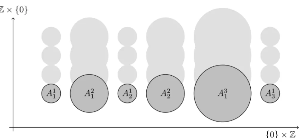
We give a last example that shows that for each set of vertices and each group, we can “blow up” this group to get a groupoid homotopy equivalent to the group having the given vertex set. This will be useful later when we want to consider a groupGtogether with a family of subgroups (Ai)i∈I as a pair of groupoids, e.g., by considering (GI,∐i∈IAi).

Definition 3.1.10. LetG be a group andC a set. We define a groupoidGC

by setting

• Objects: obGC:=C.

• Morphisms: ∀e,f∈C MorGC(e, f) :=G.

We then define composition by multiplication of elements inG, i.e., by setting for alld, e, f ∈C

MorGC(e, f)×MorGC(d, e)−→MorGC(d, f) (g, h)7−→g·h.

Example 3.1.11. For each setC, we see that{1}C is the simplicial groupoid with vertex setC.

3.1.2 The Fundamental Groupoid

For us, the main examples of groupoids, besides (disjoint families of) groups, will be given by fundamental groupoids of topological spaces. These are straightfor- ward generalisations of the fundamental group:

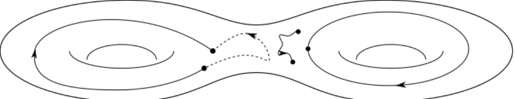
Figure 3.1: The Fundamental Groupoid – Four paths representing elements in the fundamental groupoid of the surface of genus 2.

Definition 3.1.12. Let X be a topological space and I ⊂ X a subset. We define a groupoidπ1(X, I) with object setI by setting

∀i,j∈I Morπ1(X,I)(i, j) ={c: [0,1]−→X |ca path fromitoj inX}/∼, where∼denotes homotopy relative endpoints. We define composition via con- catenation of paths. Similar to the result for the fundamental group, we see that this is indeed a well-defined groupoid, called the fundamental groupoid of X with respect toI.

We will also writeπ1(X) :=π1(X, X).

Example 3.1.13. Of course, ifX is a space andx∈X, thenπ1(X,{x}) is just the fundamental group ofX with respect to the base pointx.

Definition 3.1.14. Let (X, I) and (Y, J) be pairs of topological spaces. A continuous map f: (X, I) −→ (Y, J) induces in the obvious way a groupoid mapπ1(f) :π1(X, I)−→π1(Y, J):

(i) On objects we define π1(f) via the map f|I:I−→J

i7−→f(i).

(ii) On morphisms, we set for eachi, j∈I

Morπ1(X,I)(i, j)−→Morπ1(Y,J)(f(i), f(j)) [α]7−→[f◦α].

This defines a functor π1: Top²−→Grp.

Proposition 3.1.15. Let(X, I)and(Y, J)be pairs of topological spaces. Con- sider mapsf, g: (X, I)−→(Y, J). If f andg are homotopic, so are π1(f)and π1(g).

Proof. LetH:X×[0,1]−→Y be a homotopy betweenf andg. In particular, for alli∈I, the mapσi :=H(i, ·) : [0,1]−→Y is a path betweenf(i) andg(i).

This induces a natural equivalence ([σi])i∈I between π1(f) and π1(g): For all i, j∈I and allα∈Morπ1(X,I)(i, j) the following diagram commutes:

f(i) g(i)

f(j) g(j) [σi]

[f◦α]

[σj]

[g◦α]

Here [σi∗(f◦α)] = [(g◦α)∗σj] holds via the given homotopy.

3.2 Homological Algebra for Groupoids

In this section, we will discuss the algebraic setup to treat (co-)homology for groupoids, preparing the ground for our definition of bounded cohomology in the later sections. We introduce groupoid modules and generalise several alge- braic constructions into this context. We then discuss the Bar resolution for groupoids, define groupoid (co-)homology with coefficients and prove some el- ementary properties. The Bar resolution and the corresponding definition of cohomology is a straightforward generalisation of the group case and has been extensively studied also for groupoids, for instance [71, 75].

3.2.1 Groupoid Modules

In this section we will present our definition of a module over a groupoid, gener- alising the group case. We will then translate basic concepts for group modules, e.g. (co-)invariants, quotients etc., to this setting. Since we are mainly in- terested in bounded cohomology, we will restrict ourselves to real coefficients, though we could as well work with arbitrary coefficient rings.

Definition 3.2.1(Groupoid modules). LetGbe a groupoid. A(left)G-module V = (Ve)e∈obG consists of:

(i) A family of real vector spaces (Ve)e∈obG.

(ii) A partial action ofGonV, i.e. for eachg∈ Ga linear map ρg:V_s(g)−→V_t(g)

v7−→ρg(v) =:gv, such that:

(a) For allg, h∈ G withs(g) =t(h) we haveρg◦ρh =ρgh. (b) For alli∈obGwe haveρidi = idVi.

Definition 3.2.2(G-maps). LetG be a groupoid.

(i) Let V and W be G-modules. An R-morphism between V and W is a family (fe:Ve−→We)e∈obG ofR-linear maps.

(ii) Let f: V −→ W be an R-morphism between G-modules. We call f aG-map orG-equivariant, if for allg∈ G we haveρ^W_g ◦fs(g)=ft(g)◦ρ^V_g.

(iii) We writeG-Modfor the category ofG-modules andG-maps.

Remark 3.2.3. By definition, a leftG-module is nothing else than a covariant functor G −→R-Mod. In this sense, a G-map is just a natural transformation between such functors.

The functorial point of view is elegant, but the definition in terms of partial actions is more concrete and in direct analogy to the usual point of view in the group case. The latter definition will be our guide in the following sections, though we will also use the functorial definition to define some concepts more concisely.

Definition 3.2.4 (The trivialG-module). LetG be a groupoid. Consider the moduleR[G] := (R_e)e∈obG = (R)e∈obG. We will always endow this module with the trivialG action given by

ρg= id^R:R_s(g)−→R_t(g) for allg∈ G.

We will see more examples in later sections. In the remainder of this section, we will translate the basic concepts of group modules into the groupoid setting, concepts that we will need later in order to do homological algebra.

Definition 3.2.5. LetAandG be groupoids and letf:A −→ G be a groupoid map.

(i) LetU:G −→R-Modbe aG-module. We call theA-modulef^∗U :=U◦f the inducedA-module structure on U.

(ii) Letϕ:U −→V be aG-morphism. We define anA-morphism f^∗ϕ:f^∗U −→f^∗V,

by setting ((f^∗ϕ)e)e∈obA= (ϕf(e))e∈obA. This defines a functor f^∗: G-Mod−→ A-Mod.

Lemma 3.2.6. Let G and H be groupoids and let V be an H-module. Let f0, f1:G −→ Hbe groupoid maps andha homotopy betweenf0andf1. Then

V ◦h:f0^∗V −→f1^∗V Vf0(e)∋v7−→he·v is aG-isomorphism.

We will also use a multiplicative notation and writeh·vto denote (V◦h)(v).

Proof. By Remark 3.2.3,V◦his aG-map. Its inverse is given byV◦h, whereh denotes the inverse homotopy toh.

Definition 3.2.7. Let G be a groupoid and let V andW be G-modules. We set

Hom(V, W) ={f: V −→W |f is anR-morphism ofG-modules}

There is a canonicalG-structure on Hom(V, W) given by:

(i) Hom(V, W) = (Hom(Ve, We))e∈obG.

(ii) For allg∈ Gandf ∈Hom(Vs(g), Ws(g)) we defineg·f ∈Hom(Vt(g), Wt(g)) by setting

∀v∈Vt(g) (g·f)(v) =g·f(g⁻¹·v).

Remark 3.2.8. Another way to see this is to view Hom(V, W) as the compo- sition

G (R-Mod)² R-Mod,

(V, W) Hom

where W is the contravariant functor given by inverting morphisms in G and then applyingW.

Remark 3.2.9. Let G be a groupoid. Let f: V −→ W be a G-map and C a G-module. Then the dual map Hom(f, C) : Hom(W, C)−→Hom(V, C) (cor- responding to the family (Hom(fe, Ce))e∈obG) is again aG-map. Alternatively, we can view Hom(f, C) also as the composition of the natural transformation between (V, C) and (W, C) induced by f and the functor Hom.

This gives rise to a contravariant functor Hom(·, C) : G-Mod−→ G-Mod.

Proof. The map Hom(f, C) isG-equivariant since for allg∈ G, allv∈Vt(g)and allα∈Hom(Ws(g), Cs(g))

Hom(f, C)(gα)(v) = (gα)(f(v))

=g(α(g⁻¹f(v)))

=g(α(f(g⁻¹v)))

=g(α◦f)(v)

=g(Hom(f, C)(α))(v).

Definition 3.2.10 (Tensor products). Let G be a groupoid and letV and W be G-modules. We define thetensor product of V andW over Rto be the G- moduleV ⊗W = (Ve⊗We)e∈obG with the inducedG-structure given by setting for eachg∈G

ρg:Vs(g)⊗Ws(g)−→Vt(g)⊗Wt(g)

v⊗w7−→(g·v)⊗(g·w).

In other words,V ⊗W is the composition

G (R-Mod)² R-Mod.

(V, W) ⊗

Definition 3.2.11 (Coinvariants and Invariants). Let G be a groupoid and letV be aG-module.

(i) We define thecoinvariants ofV to be the quotient module VG = M

e∈obG

Ve/hv−g·v|g∈ G, v∈Vs(g)i.

This construction gives rise to a functorG-Mod−→R-Modby setting for eachG-mapα:V −→W

αG: VG −→WG

[v]7−→[α(v)].

In other words, the coinvariants ofV are just the canonical model for the colimit ofV:G −→R-Mod, [76, Propostion 2.6.8].

(ii) We define the invariants of V to be the R-subspace V^G of Q

e∈obGVe

defined as

V^G =n

v∈ Y

e∈obG

Ve

∀g∈G g·vs(g)=vt(g)

o.

This construction gives rise to a functorG-Mod−→R-Modby setting for eachG-mapα:V −→W

α^G:V^G −→W^G

(ve)e∈obG 7−→(α(ve))e∈obG.

In other words, the invariants ofV are just the canonical model for the limit ofV:G −→R-Mod, [76, Propostion 2.6.9].

Definition 3.2.12. LetG be a groupoid andV andW be G-modules. We call V ⊗GW := (V ⊗W)G

thetensor product of V andW overG. This construction gives rise to a func- tor · ⊗GW: G-Mod−→R-Modby setting for eachG-mapα:U −→U^′

α⊗W:U⊗GW −→U^′⊗GW [u⊗w]7−→[α(u)⊗w].

Definition 3.2.13. LetGbe a groupoid and letV andW beG-modules. Then we set

HomG(V, W) := Hom(V, W)^G.

This induces a contravariant functor HomG(·, W) : G-Mod−→R-Mod.

Definition 3.2.14 (G-Submodules). Let G be a groupoid and let V be a G- module. A G-submodule of V is a family (We)e∈obG of real vector spaces such that

(i) For eache∈obG the spaceWe is a subspace ofVe. (ii) For allg∈ G

g·Ws(g)⊂Wt(g).

ThenW carries aG-module structure by considering the restrictedG-action.

Example 3.2.15. Letf:V −→W be aG-map. Then its image (fe(Ve))e∈obG

is aG-submodule of W.

Definition 3.2.16. LetG be a groupoid andα:V −→W be a G-map. Then we call

kerα:= (kerαe)e∈obG

thekernel ofα. Clearly, kerαis a G-submodule ofV.

Proposition 3.2.17 (Quotients). Let G be a groupoid, let B be a G-module and A a G-submodule of B. Then there exists a canonical G-module structure on B/A = (Be/Ae)e∈obG such that the family of canonical projections π = (πe:Be −→ Be/Ae)e∈obG is a G-map with the following universal property:

Assume that C is a G-module and f: B −→ C a G-map such that fe(Ae) = 0 for all e ∈ obG. Then there exists a unique G-map f¯: B/A −→ C such that f¯◦π=f.

Proof.

• For all g ∈ G, we have g·As(g) ⊂At(g), hence there is a unique linear mapρg making the following diagram commutative:

Bs(g) Bt(g)

Bs(g)/As(g) Bt(g)/At(g)

ρg

ρg

πt(g)

πs(g)

This induces aG-structure onB/A.

• The projectionπ:B−→B/Ais aG-map by the definition ofρg.

• There exists a unique family of linear maps ¯f = ( ¯fe:Be−→Be/Ae)e∈obG

such that ¯fe◦πe = fe for all e ∈ obG. This map is a G-map since for allg∈ G

f¯t(g)◦ρg◦πs(g)= ¯ft(g)◦πt(g)◦ρg

=f_t(g)◦ρg

=ρg◦fs(g)

=ρg◦f¯s(g)◦πs(g). So ¯f isG-equivariant.

Remark 3.2.18. The notions of chain complex, chain contraction, resolution and so on, easily translate into the setting of groupoid modules.

Also, it is easy to see that G-Mod is an Abelian category ([76, Definition A4.2]).

3.2.2 The Bar Resolution

In this section, we will define the Bar resolution for groupoids, extending the definition for the group case. We will also present a homogeneous version and show that these two resolutions are chain isomorphic. Finally, we will introduce the Bar (co-)complex with coefficients in groupoid modules, too.

Definition 3.2.19(The Bar resolution for groupoids). LetG be a groupoid.

(i) For eachn∈N, we set

Pn(G) ={(g0, . . . , gn)∈ Gⁿ⁺¹| ∀i∈{0,...,n−1} s(gi) =t(gi+1)}.

Equivalently,Pn(G) is the set of all (n+ 1)-paths in G.

(ii) For alle∈obGconsider

Cn(G)e=Rh{(g0, . . . , gn)∈Pn(G)|t(g0) =e}i.

We define a sequence ofR-modules (Cn(G))n∈N by setting for alln∈N Cn(G) = (Cn(G)e)e∈obG

These modules carry a canonicalG-structure. TheG-action is then given by setting for allg∈ G

ρg:Cn(G)_s(g)−→Cn(G)_t(g) (g0, . . . , gn)7−→(g·g0, . . . , gn).

(iii) For eachn∈N, we define boundary maps

∂n:Cn(G)−→Cn−1(G) (g0, . . . , gn)7−→

n−1X

i=0

(−1)ⁱ(g0, . . . , gi·gi+1, . . . , gn) + (−1)ⁿ·(g0, . . . , gn−1).

These are obviouslyG-maps.

(iv) The usual calculation shows that this does indeed define aG-chain com- plex (Cn(G), ∂n)n∈N.

Remark 3.2.20. LetG be a groupoid. Consider the canonical augmentation map

ε:C0(G)−→R[G]

g7−→t(g)·1.

Then (Cn(G), ∂n)n∈N together with ε is a G-resolution of R[G]. An R-chain contractions∗ is given by theR-morphisms

s−1:R[G]−→C0(G) e7−→ide

and for alln∈N

sn:Cn(G)−→Cn+1(G)

(g0, . . . , gn)7−→(idt(g0), g0, . . . , gn).

Remark 3.2.21. The setP(G) :=∐n∈NPn(G) is just the underlying set of the nerve of the categoryG. Therefore (Pn(G))n∈Nis a simplicial set with the usual boundary maps

∂i,n:Pn(G)−→Pn−1(G)

(g0, . . . , gn)7−→(g0, . . . , gi·gi+1, . . . , gn) for eachn∈N_>0 andi∈ {0, . . . , n} and degeneracy maps

si,n:Pn(G)−→Pn+1(G)

(g0, . . . , gn)7−→(g0, . . . , gi,ids(gi), gi+1, . . . , gn).

for eachn∈Nandi∈ {0, . . . , n}. Taking the G-action into account, we could viewP(G) as a functor P(G) :G −→sSet. The chain complexC∗(G) can then be viewed as the usual chain complex associated to a simplicial set (but over the groupoidG.) We refer the book of May [55] for more on simplicial sets.

As in the group case, it is sometimes helpful to use a homogeneous resolution chain isomorphic to the Bar resolution:

Definition 3.2.22(The homogeneous Bar resolution). LetGbe a groupoid.

(i) For eachn∈N, we define aG-moduleLn(G) by setting for eache∈obG Ln(G)e=Rh{(g0, . . . , gn)∈ Gⁿ⁺¹| ∀i∈{0,...,n} t(gi) =e}i.

and defining aG-action by setting for eachg∈ G ρg:Ln(G)s(g)−→Ln(G)t(g)

(g0, . . . , gn)7−→(g·g0, . . . , g·gn).

(ii) For eachn∈N, we define boundary maps

∂n:Ln(G)−→Ln−1(G) (g0, . . . , gn)7−→

Xn i=0

(−1)ⁱ(g0, . . . ,gˆi, . . . , gn).

These are obviouslyG-maps.

(iii) The usual calculation shows that this does indeed define aG-chain com- plex (Ln(G), ∂n)n∈N.

Proposition 3.2.23. The maps

Cn(G)−→Ln(G)

(g0, . . . , gn)7−→(g0, g0·g1, . . . , g0· · · ·gn) and

Ln(G)−→Cn(G)

(g0, . . . , gn)7−→(g0, g₀⁻¹·g1, . . . , g_n−1⁻¹ ·gn) are well-defined, mutually inverseG-chain isomorphisms.