Plotting direction fields in Matlab and Maxima – a short tutorial
Luis Carvalho
Introduction
A first order differential equation can be expressed as
x0(t) =dx
dt =f(t, x) (1)
wheretis the independent variable andxis the dependent variable (ont). Note that the equation above is in normal form.
The difficulty in solving equation (1) depends clearly onf(t, x). One way to gain geometric insight on how the solution might look like is to observe that any solution to (1) should be such that the slope at any pointP(t0, x0)isf(t0, x0), since this is the value of the derivative atP. With this motivation in mind, if you select enough points and plot the slopes in each of these points, you will obtain a direction field for ODE (1). However, it is not easy to plot such a direction field for any functionf(t, x), and so we must resort to some computational help.
There are many computational packages to help us in this task. This is a short tutorial on how to plot direction fields for first order ODE’s in Matlab and Maxima.
Matlab
Matlab is a powerful “computing environment that combines numeric computation, advanced graphics and visualization” 1. A nice package for plotting direction field in Matlab (although resourceful, Matlab does not provide such facility natively) can be found athttp://math.rice.edu/∼dfield, contributed by John C. Polking from the Dept. of Mathematics at Rice University. To install this add-on, simply browse to the files for your version of Matlab and download them. Throughout this tutorial, we assume Matlab version 6.1.
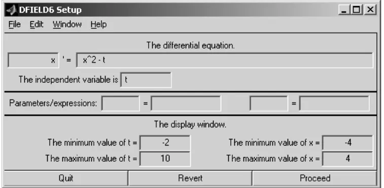
After saving the files – in our case we saved them to C:/Matlab6p1/work/ode – open Matlab and choose your working directory to be the same as the one you saved the files into. Then type dfield6. The dfield6 setup window should appear as pictured in Figure 1.
The parameters in the setup window are pretty self-explanatory. Enter the differen- tial equation, the independent variable and the ranges for the variables to be shown in the graph. Suppose we want to plot
x0(t) =dx
dt = 2x−t t, x∈(−5,5) (2)
1http://www.mathworks.com
Figure 1: Dfield setup window, right after begin called usingdfield6.
After inputing the parameters, the setup window should be similar to the one in Figure 2.
Figure 2: Dfield setup window after inputing the parameters to plot a direction field for ODE (2).
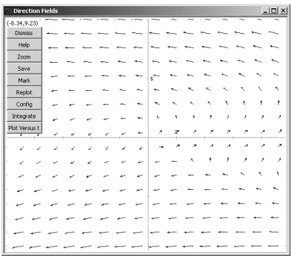
To plot the direction field, click on Proceed. The graph in Figure 3 should appear.
If you click in some point in the graph, you can see an integral curve representing the solution to the IVP (initial value problem) specified by the point. After a few clicks, we obtain a plot like the one in Figure 4. To input a different equation, simply select the setup window, update the parameters accordingly and click Proceed.
For a more throughout explanation on dfield6:
http://www.owlnet.rice.edu/∼math211/manual3/Chapter03.pdf
Maxima
Maxima is “a descendant of DOE Macsyma, which had its origins in the late 1960s at MIT. Macsyma was the first of a new breed of computer algebra systems, leading the way for programs such as Maple and Mathematica”2. Maxima is extremely powerful
2http://maxima.sourceforge.net
Figure 3: Dfield display window showing the direction field for ODE (2).
Figure 4: Dfield display window showing the direction field along with some integral curves for ODE (2).
and better suited for symbolic computations (like Maple). One point worth mentioning is that Maxima is an open source project and as such it can be freely downloaded.
Unlike Matlab, Maxima provides a nice graph facility for plotting direction fields.
We just need to tweak a few options first. The first one is to plot graphs in separate windows: in the main menu, go to Options >Plot Windows and choose Separate.
Figure 5 illustrates the procedure.
Figure 5: Maxima main window with Options>Plot Windows>Separate highlighted.
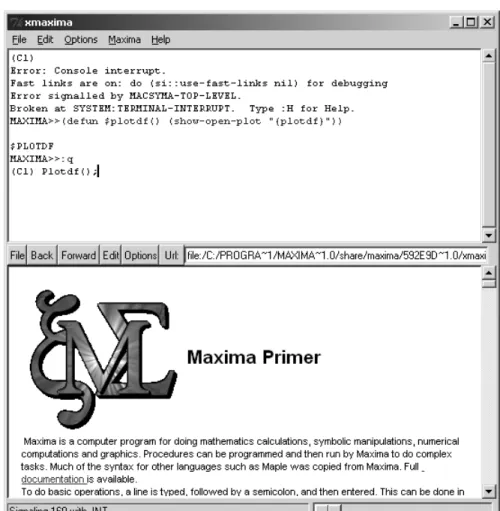
Now, the tricky part: we need to define a new function to open the direction field plot window. To do that, typeCtrl+g(or go to File>Interrupt). You should see a different prompt,MAXIMA>>. To define the new function3, type in
(defun $plotdf() (show-open-plot "{plotdf}"))
and then type:qto go back to Maxima interface. The results obtained should resemble those in Figure 6.
3This function can be saved to a file, likeplotdf.lisp, to be opened later –load("plotdf")– for better convenience.
Figure 6: Definingplotdfin Maxima.
You are now able to open the plot window by typing Plotdf();
A window like the one pictured in Figure 7 should show up.
Figure 7: Plotdf window in Maxima.
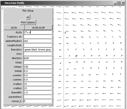
By moving the mouse pointer over the left upper corner of the window (where the current coordinates are being shown), you see the options menu (as in Figure 7). To enter the differential equation to be plotted, click on Config. On the next window, click on dy/dx to input an ODE on two variables only, and then input your equation in the dy/dx field. Also, input the range forxandy: since both must be from -5 to 5, we must set xcenter to 0, xradius to 10 and similarly for ycenter and yradius. Note that here xis the independent variable, whileyis the dependent one. After putting in the ODE corresponding to equation (2), the window obtained is illustrated in Figure 8. Now, reopen the menu and click on Replot to update the display with your new equation.
Finally, to obtain integral curves, simply click on a specific point to plot the so- lution to the ODE passing through this point. Figure 9 shows some integral curves corresponding to solutions for different points. To plot different equations, just re- peat the procedure from Config on, that is, open the menu, go to Config, type in the parameters, hit ok, reopen the menu, click on Replot.
Figure 8: Inputing parameters in the plotdf window for equation (2).
Figure 9: Plotting integral curves in plotdf.