Algorithms on Pixelized Images of Air Cherenkov Telescopes

Algorithms on Pixelized Images of Air Cherenkov Telescopes

—

Anwendung von Algorithmen des Maschinellen Lernens auf Bilder von Tscherenkov Teleskopen

M A S T E R A R B E I T

zur Erlangung des Grades eines ‘Master of Science’

im Fachbereich Physik

der Technischen Universit¨ at M¨ unchen

von Stefan Keller

Betreut von Prof. Dr. rer. nat. Susanne Mertens

Eingereicht am 09. Dezember 2019

Everything has its wonders, even darkness and silence...

- Helen Keller

Introduction 1

1 The physics of MAGIC 3

1.1 Cosmic Messengers . . . . 3

1.1.1 Sources of Cosmic γ-Rays . . . . 7

1.2 Air Showers . . . . 8

1.2.1 Ground Based Detection of Air Showers . . . . 10

1.3 The MAGIC Telescopes . . . . 11

2 Machine Learning and Neural Networks 14 2.1 Machine Learning . . . . 14

2.1.1 Supervised and Unsupervised learning . . . . 14

2.2 Neural Networks and Deep learning . . . . 15

2.2.1 Convolutional Neural Networks . . . . 19

2.3 Neural Network Tasks . . . . 24

2.3.1 Classification . . . . 24

2.3.2 Regression . . . . 24

2.3.3 Autoencoder . . . . 25

3 Machine Learning in MAGIC 26 3.1 Current MAGIC Analysis Chain . . . . 26

3.2 Hillas Parameters and Particle Parameter Reconstruction . . . . 27

3.3 MAGIC Monte Carlo Simulations . . . . 29

3.4 Neural Networks . . . . 31

3.4.1 Data Loading . . . . 32

3.4.2 Data . . . . 33

4 Results 35 4.1 Cleaning Images with the Autoencoder . . . . 35

4.2 Background rejection . . . . 38

4.2.1 Simulated Data Without Noise . . . . 38

4.2.2 Hybrid Simulations . . . . 42

4.3 Directional reconstruction . . . . 43

4.3.1 Simulated Data Without Noise . . . . 45

5 Conclusions and Outlook 48

List of Figures

1.1 Energy spectrum of cosmic rays. . . . 4 1.2 Atmospheric transmission of electromagnetic radiation by wave-

length. . . . 6 1.3 Illustration of shower development and particle interactions. . . . 9 1.4 Simulation of atmospheric air showers. . . . 9 1.5 Geometry of the Cherenkov light emission. . . . 10 1.6 Image of the MAGIC Telescopes. . . . 12 1.7 Calibrated stereo image captured by the MAGIC telescopes point-

ing at the Crab Nebula. . . . 13 2.1 Example Images of results of machine learning algorithms . . . . 15 2.2 Schematic layer structure of a neural net. . . . 16 2.3 Schematic image of the basic layout of a neuron. . . . 17 2.4 Illustration of the basic convolution process with stride 1, 3 input

channels and 6 output channels. . . . 20 2.5 Illustration of the pooling process. . . . 21 2.6 Illustration of a residual block containing two convolutional layers. 22 2.7 Illustration of a DenseNet. . . . 23 2.8 Examples of Autoencoder Applications. . . . 25 3.1 Geometrical definition of Hillas parameters. . . . 27 3.2 Illustration of a stereo position reconstruction in Imaging Air

Cherenkov Telescopes ( IACTs ) by Fruck (2015) . . . . 28 3.3 Examplary Θ ² plot from the Crab Nebula by Aleksi´ c et al. (2012) 29 3.4 Images of simulated γ-event showers. . . . 30 3.5 Example of hexagonally sampled pixels covered by a convolution

operations. . . . . 31 3.6 Individual steps for hexagonal convolution done by hexagDLy on

an examplary hexagonal grid. . . . 32 4.1 Example images cleaned with the autoencoder image cleaning. . 36 4.2 Crab Nebula images cleaned with the autoencoder image cleaning. 37 4.3 Source location distribution of simulation data. . . . 40 4.4 Energy distribution of simulated events for the background rejec-

tion. . . . 40

4.5 ROC-Curve and MVA-curve for noiseless background rejection

task. . . . 40

4.6 Binned accuracy and AUC-scores for background rejection. . . . 41

4.7 Comparison of binned noiseless background rejection. . . . 42

4.8 Comparison of binned hybrid background rejection. . . . 43

4.9 Reconstructed source location distribution of simulation data. . . 45

4.10 Θ ² plot for the directional reconstruction neural network. . . . . 46

4.11 Binned Θ ² plot for the directional reconstruction neural network. 46

4.12 Binned direction reconstruction results and comparison. . . . 47

List of Tables

4.1 Architecture of the autoencoder for image cleaning. . . . 38 4.2 Architecture of the ResNetHG-45 used for the gamma-hadron

separation task. . . . 39

4.3 Architecture of the directional reconstruction DenseNetHG-94. . 44

AGN Active Galactic Nucleus . . . 7

AN Artificial Neuron . . . 17

AUC Area Under Curve . . . 41

CMB Cosmic Microwave Background . . . 5

CNN Convolutional Neural Network . . . 19

CORSIKA Cosmic Ray Simulations for Kascade . . . 29

CTA Cherenkov Telescope Array . . . 11

DenseNet Dense Convolutional Network . . . 21

EAS Extensive Air Shower . . . 26

GAN Generative Adversarial Network GRB Gamma Ray Burst . . . 1

H.E.S.S. High Energy Stereoscopic System . . . 11

IACT Imaging Air Cherenkov Telescope . . . ii

LST Large Size Telescope MAGIC Major Atmospheric Gamma Imaging Cherenkov Telescope . . . 1

MARS MAGIC Analysis and Reconstruction Software . . . 26

MC Monte Carlo . . . 26

ML Machine Learning. . . .24

NN Neural Network . . . 18

PReLU Parametric Rectified Linear Unit . . . 17

ReLU Rectified Linear Unit . . . 17

RF Random Forest . . . 26

RNN Recurrent Neural Network . . . 24

ResNet Residual Network . . . 21

ROC Receiver Operating Characteristic. . . .38

SGD Stochastic Gradient Descent . . . 18

SNR Supernove Remnant . . . 7

MVA Multi Variate Analysis . . . 38

VERITAS Very Energetic Radiation Imaging Telescope Array System . . . . 11

WIMP Weakly Interacting Massive Particle . . . 8

Glossary

Accuracy Percentage of predictions that were classified correctly. For a binary classification the accuracy is defined as Accuracy = True Positives + True Negatives

Total Number of Examples

AUC Evaluation metric for classifiers that describes the area under the ROC- curve. Considers all classification thresholds.

Backpropagation Updating the network parameter based on the gradient cal- culated based on the network output on training data.

Batch Collection of training samples for the estimation of the gradient once at each iteration.

Batch Size Number of training samples used in training for the estimation of the gradient at each step.

Classification Threshold A convolution in machine learning is a function applied to a matrix that mixes the filters and the input matrix.

Convolution A convolution in machine learning is a function applied to a matrix that mixes the filters and the input matrix.

Epoch Parameter that describes the number of times all the training data is used once.

False Positive Rate The false positive rate is a metric for evaluating the frac- tion of positive classifications that were classified wrongly.

Feature A property of the data that is used in machine learning as an input value.

Fully Connected Layer A convolution in machine learning is a function ap- plied to a matrix that mixes the filters and the input matrix.

Hyperparameter Parameter that is set before the training of a machine learn- ing algorithm and not changed during training.

Label Target value of the data that the machine learning algorithm has to predict.

Learning Rate Parameter that describes the step size in the optimization al-

gorithm.

Off Data Data captured in an observation of an area of space that does not contain any known high energy γ-ray sources, i.e. pure proton datasets or datasets with an insignificant amount of γ events.

Overfitting A machine learning algorithms overfits if it adjust too closely to the training data to generalize on new data.

Random Forest Machine learning algorithm that is based on a multitude of decisison trees. The output of all trees is averaged to get the final decisi- sion.

ROC Curve Curve that plots the False Positive Rate against the True Positive Rate at different classification thresholds to evaluate the performance of a classification machine learning algorithm.

Softmax Probability function in multi class classification algorithms. Normal- izes the output values of a neural network.

Stride Distance in grid spaces that the convolution filter moves between each convolution step.

True Negative Correct prediction of negative class in binary classification.

True Positive Correct prediction of positive class in binary classification.

True Positive Rate The true positive rate is a metric for evaluating the frac-

tion of positive classifications that were classified correctly. Also called

recall.

For millennia, humans have looked at the sky and wondered. Nowadays we got a pretty good picture of what lies beyond our own planet earth. Interstellar travel is not possible due to us being confined by the human lifespan and tech- nology so that we are unable to wander further than our own planet and nearby solar system. However, science can help us expand our knowledge of the uni- verse and escape the realms of our own physical confinement by utilizing cosmic messengers. The messengers neutrinos, cosmic rays, photons and only for a few years yet gravitational waves allow us to get an understanding of our universe humans could not have imagined 100 years ago and we might not imagine what discoveries the future might reveal. Especially the electromagnetic spectrum with its wide range of energies allows us the study of many different parts of our universe.

From the low energy radio waves, with which the first picture of a black hole was taken or which constitutes the cosmic microwave background, star formation bright in the infrared, the light of stars from the optical to UV and x-rays of compact stellar remnants to gamma ray bursts, the universe presents itself to us in many different ways. Especially the γ-ray astronomy enables us a deep look into violent high energy events in our universe. Just recently in January 2019, the Major Atmospheric Gamma Imaging Cherenkov Telescope ( MAGIC ) telescopes were able to detect TeV emission from a Gamma Ray Burst ( GRB ) and therefore confirm the existence of a high energy component in GRB afterglows with more than 50 standard deviations.

Using multiple high-tech telescopes that operate with different particles in dif-

ferent wavelength ranges and concluding a new scientific discovery with extreme

accuracy could not have been imagined 100 years ago. This major feat shows

what can be possible when science and technology work hand in hand, further

advancing the boundaries of what we know and think is possible. Another tech-

nology that shows the benefits of science and technology working hand in hand

is machine learning. Although it is not a new field of research, machine learn-

ing has opened new possibilities in the last few years that can help us in many

different ways. In science and data analysis, algorithms that can learn to fulfill

tasks without being explicitly told how to do so can help immensely, as many

tasks are hard to do with explicit instructions. The availability of computing

power has propelled the development of neural networks and deep learning in

the last few years and it is still propagating with new developments nearly every

Introduction

day. It is often seen as one of the most important technologies of the future and already severely influences our daily life. Big companies like Google and NVidia invest heavily in this technology to provide customers a new and better experience as well as advancing what is possible even further. Machine learning is also finding its way into science, albeit slowly as there are still many ques- tion to answer like error propagation and the applicability of neural networks on observation data after being trained on simulation. Therefore, we need to continue experimenting with new technologies and apply them to the problems of our everyday life and in science.

This thesis’ objective is the development and testing of machine learning algo-

rithms for the MAGIC telescope analysis. In the MAGIC experiment, current

analysis is based on a hillas parametrization of shower images by fitting a el-

lipses onto the images. However, this disregards all the information that might

contain useful information for the reconstruction of particle properties which is

encoded in the exact locations and brightness information of the camera pix-

els. The use of pixelized images in the analysis process and whether the usage

of pixel information with neural networks instead of parametrized images im-

proves and speeds up the analysis is tested. Chapter 1 and Chapter 2 describe

some background on the physics involved, the MAGIC telescopes and machine

learning, especially neural networks. Chapter 3 reports on the current analysis

methods in MAGIC and the new approach, followed by the results in Chapter 4

where the developed algorithms will be applied to simulated and real data. The

last Chapter 5 features a summary of the thesis and the outlook.

If not indicated differently, this chapter is based on the book Cosmic Rays and Particle Physics by Gaisser et al. (2016).

1.1 Cosmic Messengers

As we cannot travel to distant stars and are bound to our planet and nearby solar system, the studying of the universe requires us to use cosmic messengers.

Due to the nature of the different particles, each cosmic messenger particle has its own properties and originates from other processes. This enables us to study different aspects of our universe in further detail. In the following, the four major cosmic messengers charged particles, neutrinos, gravitational waves and photons are summarized in short.

Cosmic Rays

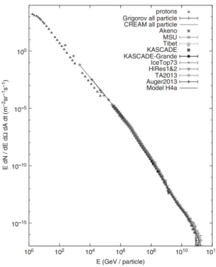
Cosmic rays are charged particles with mostly relativistic and ultra relativis- tic energies. Charged particles that are produced and accelerated in galactic and extragalactic sources are primary cosmic rays. They consist out of mostly protons (∼ 90 %), α-particles (9 %) and heavier nuclei. Secondary cosmic rays are charged particles that are created in collisions of primary cosmic rays with the particles in the interstellar medium or our atmosphere. They consist of charged particles like anti-particles such as anti-protons and positrons, but also electrons and protons as well as other hadrons and leptons can be produced in these collisions. About 1000 cosmic ray particles hit the Earths’ atmosphere per square meter per second as stated by Gaisser et al. 2016. The energy spectrum of cosmic rays hitting the Earth is shown in figure 1.1.

The spectrum follows an inverse power law distribution of about E ⁻ 3 and shows

two small kinks and a cut-off, the ”knee” at about 3 × 10 ⁶ GeV and the ”an-

kle” at about 3 × 10 ⁹ GeV as well as a sharp drop off in the flux at about

5 × 10 ¹⁰ GeV. The cause of this drop off is not yet known, but there are theo-

ries that say that it might be due to source depletion i.e. that cosmic-rays can-

not be accelerated to higher energies or due to the Greisen–Zatsepin–Kuzmin

limit, where this drop off can be explained by the interaction of cosmic rays

1.1. Cosmic Messengers

Figure 1.1: Energy spectrum of cosmic rays.

Energy spectrum of cosmic rays. Image by Gaisser et al. (2016).

with the Cosmic Microwave Background ( CMB ) (Greisen 1966). There are still very few cosmic ray particles with energies up to about 10 ²⁰ GeV. Most cosmic rays originate from our galaxy but outside of our solar system and the few cos- mic rays that originate in our solar system can be associated with violent solar events. Only cosmic rays with very high energies are from outside our galaxy as they could escape their own originating galaxies’ magnetic fields. Due to their charged nature, cosmic-ray particles get deflected by magnetic fields and cannot be used to trace them back to their source. Cosmic rays can either be detected directly by experiments like AMS-02 onboard the International Space Station or balloon experiments, or indirectly by detecting the secondary parti- cles produced in hadronic particle showers, caused by cosmic rays hitting Earths’

atmosphere.

Cosmic Neutrinos

Neutrinos are light, uncharged leptons that only interact via the weak force.

Their low interaction cross sections and low natural flux make them hard to detect and current experiments like Ice-Cube or Super-Kamiokande have to use vast detector volumes, in which the neutrinos can interact with the detector material. These interactions produce Cherenkov light that is then detected with photo multiplier tubes. Due to their uncharged nature and low interaction cross section, neutrinos are not deflected by galactic magnetic fields and rarely interact on their way to us. This makes them ideal for source reconstruction.

Recent discoveries showed that neutrinos have mass and undergo flavour mixing, i.e. a neutrino changes its flavour over time. The standard model of Cosmology says that primordial neutrinos that make up the cosmic neutrino background were created one second after the big bang. Detecting these neutrinos could give more insight into the origin of our universe, but the detection of these neutrinos might even in the future will always remain impossible due to their low temperature.

Gravitational Waves

Gravitational waves were first predicted by Einstein (1916) as waves in space-

time, caused by non rotational symmetric accelerating matter. Gravitational

waves squeeze and stretch space time along their propagation direction. The

first direct detection was achieved more than a hundred years later by the LIGO

Collaboration, using two light interferometers located 3002 km apart (Abbott

et al. 2016). Albeit their relatively recent discovery, quite a few sources of gravi-

tational waves from colliding massive objects like black holes and neutrons stars

were already discovered. With the ever increasing sensitivity of new technolo-

gies and more light interferometry observatories being built around the Earth,

gravitational wave astronomy has just started and will offer an even deeper look

into our universe.

1.1. Cosmic Messengers

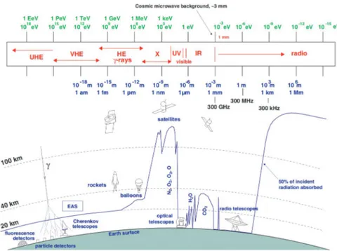
Figure 1.2: Atmospheric transmission of electromagnetic radiation by wave- length. A detector can receive half the incoming radiation for each wavelength at the height indicated by the continuous line.

Cosmic γ-Rays

From the radio via infrared, visible and ultraviolet light to x-rays and γ-rays,

photons cover a huge range of observable frequencies, all with different detection

methods, requirements and observation possibilities. As seen in figure 1.2, only

visible light and radio waves are transmitted by the atmosphere and can be

directly observed from Earths’ surface. Long radio waves, infrared and most

wavelengths shorter than visible light are best observed from space as they are

blocked by the atmosphere. At very high energies however, the photon flux is

very small. Satellite-based experiments do not have the required detector area to

measure these fluxes and are therefore currently not appropriate for the highest

energy ranges. To detect these high-energy γ-rays, Earth-based detectors are

used using electromagnetic air showers, caused by high-energy γ-rays interacting

with the Earths’ atmosphere. These showers contain charged particles which

move faster than the speed of light in air and therefore emit Cherenkov light,

that can be detected by specially designed IACTs . More about the creation of

cosmic showers is written in section 1.2 and about IACTs in section 1.3.

1.1.1 Sources of Cosmic γ-Rays

High energy cosmic γ-rays are produced in a lot of astrophysical processes and environments. The major source types are listed in the following.

• Supernova Remnants A supernova can occur, when a massive star runs out of fuel or a white dwarf reaches the Chandrasekhar mass either due to mass accretion from a companion star or from a merger with another white dwarf (Ken’ichi Nomoto et al. 2018). These supernova explosions expel huge amounts of stellar material with supersonic velocities that hit the interstellar medium and form a shock wave ahead of the ejected material, which forms the Supernove Remnant ( SNR ). The interaction of charged particles with the turbulent magnetic fields caused by the shock front can produce high energy gamma rays.

• Pulsars After the explosion of a massive star in a supernova, a rapidly rotating neutron star with strong magnetic fields can be the remnant.

Such neutron stars emit a beam of strong electromagnetic radiation that appears pulsed due to its rotation. This beam can be used for exact time keeping.

• Pulsar Wind Nebula A pulsar wind nebula can be caused a pulsar inside a supernova remnant. Due to the strong magnetic field of the ro- tating pulsar, charged particles are accelerated to relativistic velocities that compose the pulsar winds.

• Microquasar

A microquasar is a binary system out of a stellar mass black hole and a star. The black hole accretes matter from the star and an accretion disk forms around the back hole as well as trans relativistic jets. Due to friction, the accretion heats up and emits high energy x-rays and γradiation.

• Active Galactive Nuclei

Active Galactic Nuclei ( AGN ) are the compact and luminous centers of some galaxies, that can not be explained by a superposition of stars. They are theorized to be super massive black holes at the center of Galaxies, which accrete huge amounts matter that forms an accretion disk around the black hole. Due to friction, the accretion disk heats up and radiation is emitted. Depending on the orientation of the AGN to the observer, different parts of the emitted radiation can be observed. AGN can also form jets which emit photons with the highest energies observed yet in the TeV range. If the jet is directed at Earth, the AGN is called Blazar.

• Gamma Ray Bursts GRB are powerful explosions, that send out strong γ-radiation that can last from few milliseconds to about 100 s. After the initial burst, an afterglow can be observed in shorter wavelengths. The sources of GRB are theorized to be supernovae or neutron stars mergers.

In 2019, the MAGIC Telescope detected TeV photons undoubtly emitted

1.2. Air Showers

by a GRB for the first time.

• Dark Matter Dark matter could consist of Weakly Interacting Massive Particles ( WIMPs ), that can annihilate into standard model particles, emit- ting high energy γ-rays in the final state.

1.2 Air Showers

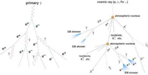
If a very high energy γ-ray interacts with the atmosphere, it can induce an extensive electromagnetic air shower. In the first interaction, the γ-ray pro- duces an electron-positron pair via pair production, which then emits γ-rays via Bremsstrahlung. These γ-ray photons will again undergo pair production and cascade further until the particles’ energy is low enough for other processes (Compton scattering for photons and ionization for electrons and positrons) to be dominant. The point in the shower development, where the amount of par- ticles present is at a maximum depends on the incoming photons’ energy. The highly relativistic electrons and positrons produced in the electromagnetic air shower produce Cherenkov light while propagating through air as described in section 1.2. The produced Cherenkov light is also dependent on the height of shower development, as it depends on the density of air. The lateral size of the electromagnetic shower is small and the shower axis mostly coincides with the direction of emitted photons.

A very high energy proton that interacts with a proton or nucleus in the at- mosphere can induce an extensive hadronic air shower. The first interaction produces charged and neutral mesons and baryons, to which all the energy of the initial nucleon or proton is transferred. The secondary particles continue and interact again to produce more secondary hadrons until their energy is lower than the interaction threshold. Unstable hadrons can also decay with an increasing probability as the energy decreases. The decay of neutral pions into two γ-rays and the decay of charged pions into muons and neutrinos which then create electromagnetic subshowers. All subshowers produce Cherenkov light, which can be detected by IACTs. The showers caused by charged cosmic rays are much broader than the showers caused by photons or charged leptons (Stanev 2010). Figure 1.3 illustrates the particle interactions and the shower development of electromagnetic and hadronic air showers.

Cherenkov radiation

Cherenkov radiation is electromagnetic radiation caused by charged particles

that move with a velocity v _p > c _n through a non conducting, dielectric medium

with refractive index n and speed of light in the medium c _n defined by equation

1.1. It was discovered in 1934 by Pavel Cherenkov.

Figure 1.3: Illustration of shower development and particle interactions for a electromagnetic air shower (left) and a hadronic air shower (right) by Wagner (2006).

Figure 1.4: Simulation of atmospheric air showers in CORSIKA at 1 TeV initial

particle energy each. a) shows a photon shower and the b) shows a proton

shower. The left part shows the shower in the x-z plane and the right images

show the shower in the x-y plane. Images by Heck (2019).

1.2. Air Showers

Figure 1.5: Geometry of the Cherenkov light emission.

c n = c 0

n (1.1)

As the charged particle travels through the medium, it is polarized. As the medium relaxes, light will be emitted under the angle Θ Cherenkov according to equation 1.1. Only the coherent light travels long enough to be visible. Figure 1.5 shows a schematic image of the emission geometry.

cos(Θ Cherenkov ) = c nv p

(1.2)

1.2.1 Ground Based Detection of Air Showers

Direct Detection of Shower Particles

The Pierre Auger Observatory is a ground based hadronic shower detector de-

signed for incident particles with energies above 1 × 10 ¹⁷ eV. It is located in Ar-

gentina and covers a surface area of about 300 km ² with 1660 water Cherenkov

detectors on the ground as surface detectors and four fluorescence telescopes

that cover area above the surface detectors. The surface detector array de-

termines the secondary particles of the showers’ electromagnetic, muonic and

hadronic components by detecting the emitted Cherenkov when a particle en-

ters one of the detectors. The fluorescence detectors observe the fluorescence

and Cherenkov light emitted by the showers’ secondary particles to analyze the

longitudinal development of the shower. The energy threshold of incident par-

ticles of the Pierre Auger Observatory is at about 10 × 10 ¹⁷ eV and therefore

only viable for the ultra high energy cosmic rays. (Castellina 2019)

Detection of Cherenkov Light emitted by Atmospheric Showers The Cherenkov light, emitted by the secondary particles in electromagnetic showers and subshowers can be detected in a wide area. The light is mostly in the optical and UV bands. These flashes only last a few ns.The amount of light as well as the spatial and angular distribution of the emitted Cherenkov light depends on the initial particles’ parameters, which allows the reconstruction of the particles incident direction and energy. The reconstruction of the particles parameters is normally done based on an adjusted hillas parametrization by Hillas (1985). More details about the reconstruction in section 3.2. The current major Imaging Air Cherenkov Telescopes are the MAGIC telescope on the island of La Palma, Spain, the High Energy Stereoscopic System ( H.E.S.S. ) in Namibia and the Very Energetic Radiation Imaging Telescope Array System ( VERITAS ) Telescope Array in southern Arizona, USA. The next step in the IACT world is the planned Cherenkov Telescope Array ( CTA ) Observatory, consisting of two Array sites: CTA North on La Palma, Spain and CTA South in Paranal, Chile.

1.3 The MAGIC Telescopes

The MAGIC Telescopes are two Air Cherenkov telescopes with a diameter of 17 m located on the Canary island of la Palma. They are part of the Roque de los Muchachos Observatory at a height of about 2200 m above sea level on the hillside of the volcano with the same name. The telescopes are 85 m apart.

The ∼ 240 m ² parabolic reflective areas consist of 246 1 m ² individual mirrors, each individually controllable with an actuator. The Magic 1 telescope was taken into operation in 2004 and upgraded in the years 2011-2012 to match the Magic 2 telescope, which was taken into operations in 2009 (Aleksic et al. 2014).

Nowadays, if possible, both telescopes always take data in stereo mode.

Camera

The cameras consist of 1039 hexagonal pixels, each with a diameter of 1 inch, arranged in a circular shape. Each pixel consists of a Photo-multiplier tube connected to the read-out electronics, that amplifies and converts the signal from analog to optical, which is then sent via optical fibers to the counting house.

The camera is operated so that observations during moonlight are possible.

Each telescope camera has its own triggering mechanism, that depends on the

amount of photons that hit a pixel and its surrounding area. A stereo image will

only be saved if both Magic cameras report a trigger signal. Additionally, an

image of the background is captured at 25 Hz. These pedestal images show the

electronic noise induced by the camera and read out electronic and the night

sky background without the Cherenkov photons from an atmospheric shower

1.3. The MAGIC Telescopes

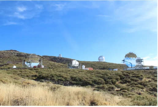
Figure 1.6: Image of the MAGIC Telescopes. The MAGIC 1 and MAGIC 2

telescopes can be seen on the left and in the middle, the LST 1 telescope on the

right. Photo by Lea Heckmann.

Figure 1.7: Calibrated stereo image captured by the MAGIC telescopes pointing at the Crab Nebula.

that normally trigger the camera. The output of the telescope contains a single

channel wave form for each pixel from which the number of photo electrons per

pixel can be reconstructed. A stereo image captured by the telescope can be

seen in figure 1.7.

2 Machine Learning and Neural Networks

This is section is based on Goodfellow et al. 2016 if not indicated differently.

It describes machine learning and neural networks as it is needed in this thesis and does not give a complete overview over the techniques used by the machine learning community.

2.1 Machine Learning

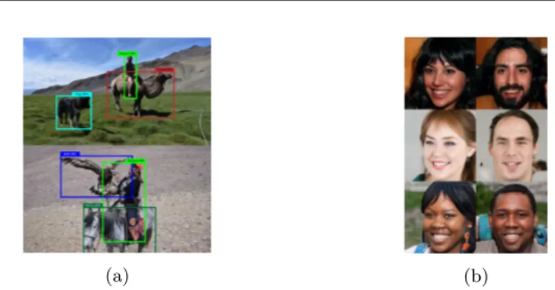
Machine learning is a form of applied statistics, which describes algorithms that learn to perform a task without explicit instructions given by the user. By inputting data and evaluating its performance at the given task on this data with continued adjustment of internal parameters its ability to perform the given task is learned. The continued adjustment of internal parameters is based on the gained experience of the algorithm during training. This improves its performance at the given task. In the last few years, especially deep learn- ing techniques that feature algorithms with millions of learned parameters have seen increased usage and developments due to technological advances and in- creased available computing power available to everybody. Especially in image and speech recognition tasks, neural networks have recently seen increased ap- plication in companies like Google, NVidia, SAP, Tesla and many more, that also actively develop machine learning frameworks and invest hugely in ma- chine learning research. Famous machine learning algorithms like You Only Look Once (YOLO), a state of the art real time object recognition library by Redmon et al. (2018) or StyleGAN by Karras et al. (2018) that creates realistic human faces of people that do not exist. This area is often seen as one of the most important technologies for the future. In science however, it is still not common to use machine learning algorithms and neural networks.

2.1.1 Supervised and Unsupervised learning

In machine learning, algorithms are roughly divided in supervised and unsuper-

vised learning algorithms. In supervised learning, each example of the input

data set contains its corresponding label. For example, a handwritten digit

(a) (b)

Figure 2.1: Example Images of results of machine learning algorithms (a) YOLO real time object recognition neural network by Redmon et al. (2018) and (b) StyleGAN by Karras et al. (2018), a GAN that produces nearly indistinguishable images of human faces.

recognizer data set contains the number displayed in the image as label. In a simple case, supervised learning tries to match each input data vector x to its corresponding label y. If only some of the data is labeled, the problem sits be- tween supervised and unsupervised learning as semi-supervised learning. This is often due to time or money constraints as labeling data is a time consuming task in real world applications. In Unsupervised learning, the algorithms experience the input data without corresponding labels. Instead, the unsupervised learning algorithms are expected to find structures and patterns in the given data while preserving most information given and being limited by a constraint. There is no supervisor that tells the algorithms explicitly what is right and what is wrong, but other algorithms and neural networks can serve as a constraint, e.g.

by checking the outputs’ accuracy. Unsupervised learning algorithms for exam- ple can be used for clustering, where data is put into related groups without predefined groups and characteristics or finding associations between different data sets. While the difference between between supervised and unsupervised learning is not rigidly defined due to some ambiguity in the choice of whether a value is a feature or a label, in most cases unsupervised learning is defined as ma- chine learning based on input data, that was not annotated by humans whereas supervised learning is mostly based on data, annotated by humans.

2.2 Neural Networks and Deep learning

A neural network is a special subset of machine learning algorithms. Although

neural networks were around since the 1940s, the technology gained interest

in the last years due to recent developments and the ever increasing available

computing power to everyone, that allow the training of deep neural networks on

relatively short timescales. Due to their non linear nature, neural networks can

2.2. Neural Networks and Deep learning

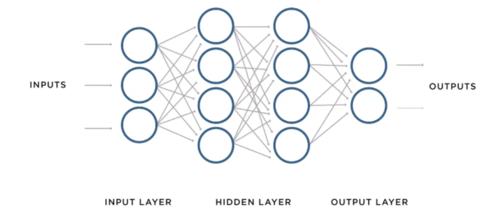
Figure 2.2: Schematic layer structure of a neural net. Each layer, ordered from the left to the right consists out of multiple neurons which are connected to each neuron of the previous where they receive their input from and following layer, where they send their output to.

learn even complex, non linear statistical distributions and especially in image and speech recognition, neural networks can achieve a high accuracy.

Basic Structure of a Neural Net

The most central neural network in deep learning is the feed forward neural network, that is supposed to approximate some function f ^∗ by feeding the input data x forward through the network and approximating its output y = f (x).

Most commonly, these networks consist of multiple functions f ¹ , f ² , ..., that form a network along the structure of y = f ⁽ⁿ⁾ (f ⁽ⁿ⁻¹⁾ (...f ⁽²⁾ (f ⁽¹⁾ (x))). Here, f ⁽¹⁾ is the input layer of the network containing the input data, f ⁽ⁿ⁾ is the output layer and the other layer in between are the hidden layers. A schematic overview of a simple neural net can be seen in Figure 2.2, where each layer consists out of multiple neurons as described below, that are connected to each neuron of the previous, where they receive their input from and the following layer, where they send their output to.

By feeding the training data x in supervised learning algorithm with different

labels y into the neural network, we want the network function f to match

the underlying distribution function f ^∗ . At each point x in the training data,

the network should compute outputs that are close to the corresponding labels

y. The data does not specify what the function should be and how each layer

should be used, this has to be inferred by the algorithm. The layers between the

input and output layer are called hidden layers because their inner weights and

biases are learned and not defined. The width of the neural net is the amount

Figure 2.3: Schematic image of the basic layout of a neuron.

of hidden layers it contains.

Each layer in the neural net consists out of a vector of so called neurons or Artificial Neuron ( AN ). These are loosely based on the neurons in the brain but do not model the brains function. They are rather designed to achieve statistical generalization. Each neuron receives the values x i from multiple inputs i, each with its own weight w i and calculates z according to the linear equation 2.1, where b is the bias of the neuron.

z(x) = X

i

w _i · x _i + b (2.1)

The neuron then computes its output f neuron based on equation 2.2, where g is the activation function.

f neuron = g (z) (2.2)

The result of the neuron y is then propagated to each neuron in the next layer,

where it is used as an input. This neural nets’ non linearity depends solely on

the activation function g. A linear activation only allows for the estimation of

linear statistical distributions, while a non linear activation function g allows for

even complex, non linear distributions to be predicted by the neural network. A

schematic image of a neuron can be seen in Figure 2.3. The most common acti-

vation function in the past was the Sigmoid (g sigmoid (z) = _1+e ¹

) function, but

nowadays the recommended function Rectified Linear Unit ( ReLU ) (g ReLU (z) =

max(0, z)) or one of its variations (LeakyReLU g LeakyReLU (z) = max( ∗ z, z)

or Parametric Rectified Linear Unit ( PReLU ) g P ReLU (z) = max(α ∗ z, z), where

α is a learnable parameter) due to their piece wise linearity, which conserves a

lot properties of the linear activation functions, while being non linear. This

is important, because many properties of linear based models favor them at

generalizing and make them easy to optimize with gradient based methods, but

as they can only approximate linear functions, stepwise linear functions unite

the best of both worlds. The amount of neurons and layers in a neural network

2.2. Neural Networks and Deep learning

is one of the main parameters that changes its results. In principle, the more neurons and layers a neural network has, the more features can be extracted and the more complex the processed information can be but the more parameters it has the more data it needs to converge. Deeper networks with not enough data can also be prone to overfitting, where the neural net loses generalization performance and adjusts too much to the training data.

Training the Network

The training of a neural network follows a simple, but powerful principle. First, the forward propagation is executed, which means that the training data is input into the network and the outputs are calculated. The loss, that is the difference between true value of the input data y true and output value y output according to a cost function is then calculated. Depending on the problem that is to be solved, the loss function has to be chosen accordingly. Two examples for loss functions, L ¹ that calculates the absolute derivations and L ² that calculates the squared deviations are given in equations 2.3 and 2.4.

S L1 = Σ ⁿ _i=0 |y true − y predicted | (2.3) S L2 = Σ ⁿ _i=0 |y true − y predicted | ² (2.4) The cost information then flows backwards through the net in the back-propagation.

Here the weights and biases of the net are adjusted to minimize the loss. The most famous algorithm for back-propagation is the Stochastic Gradient De- scent ( SGD ). It calculates the negative gradient of the cost function and adjusts the weights and biases depending on the calculated gradients. Executing this on all training examples at once yields a good result for the gradient, but is compu- tationally expensive. Therefore, mostly the training is done in mini batches, i.e.

selecting a specific number of random samples of training images, executing the

forward and back propagation and updating the nets’ parameters for each mini

batch. This leads to a better estimation of the gradient than backpropagating

for each event, but might harm its generalization performance. Passing through

the whole training data once in mini batches is one epoch. The Neural Net-

work ( NN ) is trained for multiple epochs, the exact number depending on the

task. Neural networks are very specific to the problem and there is no general

method of choosing the network architecture and the hyperparameter, i.e. the

parameters set before training begins that do not change during training. Most

networks are a product of changing and experimenting with the hyperparameter

and the network structure and comparing the results. For experimenting, it is

important to not get biased on the performance on the training data, as the

data ”wears out” with repeated use and its expressiveness gets reduced. There-

fore, most training is done with data split into 3 subsets: A training set used

for training, a validation set used for comparing the different net architectures

and hyperparameter and a until the end unused test set for determining the performance on the chosen network architecture and hyper parameters.

2.2.1 Convolutional Neural Networks

For processing data in a grid-like structure like images, a special kind of neural net is used, the Convolutional Neural Network ( CNN ). As the name indicates, the mathematical operation “convolution“ is used, although it is not exactly the kind defined in mathematics or physics.

Convolutional Layers

The main advantages of convolutional layers are equivariance, sparse interac- tions and parameter sharing: The convolutional layers are equivariant, i.e. if the input changes, the output will change in the same way. Furthermore, the kernel in a convolutional layer is normally much smaller than the size of the in- put. Not every element in a the convolutional layer is connected to every other element and therefore interactions are sparse and the computation time of the matrices is reduced. Closely related to the sparse interactions is the parameter sharing. It means that the same parameters are used for multiple functions in the model. Each weight of the kernel is used at nearly every location of the input. This reduces the data storage requirement.

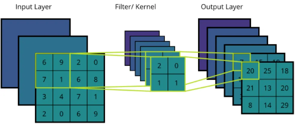
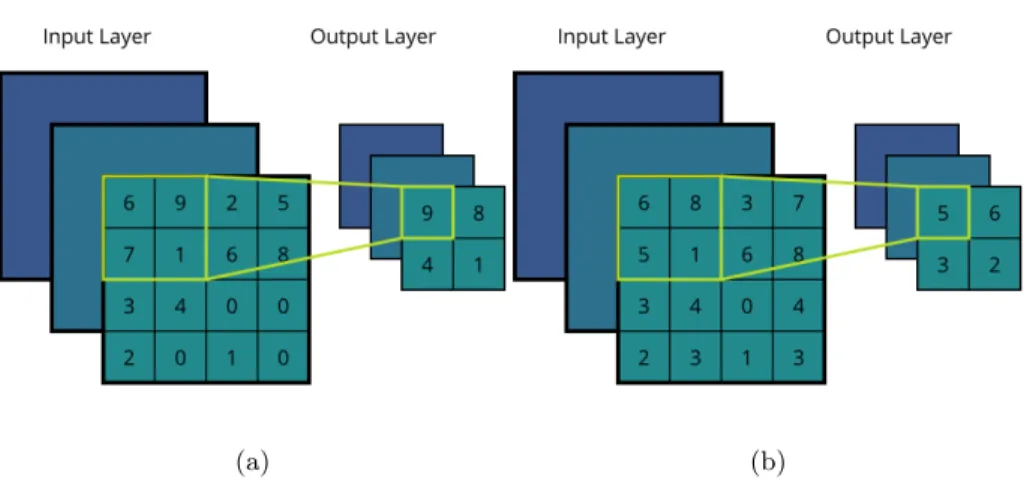
A convolution operation in the field of neural networks does not exactly match the definitions in mathematical literature. In many cases, the input data can be viewed as 3-dimensional tensors, with 2 indices indicating the spatial coordinate and the third index indicating the channel, i.e. for a RGB color image, as is standard in most computer applications, the 3 channels in the image are for the colors red, green and blue. In neural networks, a convolution operation typically applies multiple convolutions in parallel to extract multiple different features from the image, as each kernel can only extract one feature and produce one feature map. This increases the amount of channels that are output. A schematic presentation of a convolutional layer can be seen in figure 2.4.

The output of the convolution operation can also be down sampled by skipping

over some position. This is done by strided convolutions, where the stride

defines the distance between the locations, where the convolution operation is

applied. Furthermore, the image can be padded before the convolution operation

is applied. This increases the output size and can prevent the reduction of the

images’ spatial size due the natural size reduction of convolution operations as

each convolution operation with a kernel bigger than 1×1 reduces the spatial size

of the unpadded input. The padding typically defaults to zero, as it normally

does not influence the output of the convolution operation.

2.2. Neural Networks and Deep learning

Figure 2.4: Illustration of the basic convolution process with stride 1, 3 input channels and 6 output channels.

Pooling layers

In a CNN, a typical layer consists of three stages. The first stage creates a linear activation using one or several convolutions followed by the second stage, the nonlinear activation function. The third stage consists of a pooling function.

The pooling function computes a summary statistic of each locations’ nearby output areas. It induces some translational invariance into the data. This makes the pooling function especially useful if it is not important where exactly the feature is located, but whether it is present or not. The pooling function can also reduce the spatial size of the data and therefore reduces the computing required in the next layer. It can also adjust the network to use different sized input data, because the fully connected layers that typically follow the convolutional layers have a fixed input size. Most commonly, the pooling functions are max pooling, where only the maximum value in the pooling area is retained or average pooling, where the output is the average of all pixels in the pooling area. Figure 2.5 illustrates the pooling layer on two typical pooling operations, max pooling and average pooling.

Radford et al. 2015 shows, that a convolutional layer with increased stride can re- place a pooling layer without losing accuracy and even improving results.

Residual Blocks

A residual neural network is a neural network architecture shown by He et al.

(2015). It contains shortcut connections that allow the network to easily model

identity mappings with small perturbations. This improves deeper networks

(a) (b)

Figure 2.5: Image (a) shows basic max-pooling on a location of the grid. Image (b) shows a basic average pooling that outputs the average of the neighbourhood around the pooled location.

and helps to prevent the degradation problem, i.e. deeper networks show higher errors than their shallower counterparts, which is not caused by overfitting but problems of the optimization. The residual network is based on the assump- tion, that if a couple of stacked layers can approximate the underlying function H (x), the residual functions F (x) := H (x) − x can also be asymptotically ap- proximated by the layers. Therefore, the layer try to map the function F (x)+x, which is equivalent to the original formalisation, but is easier to train, especially for deeper networks. An illustration of a residual block can be seen in figure 2.6.

DenseNet

A Dense Convolutional Network ( DenseNet ) is a network architecture proposed by Huang et al. (2018) for improved flow of information and gradients as well as reduction of parameters and better training performance for deeper networks.

A problem of the Resnet architecture is the high amount of parameters and

that layers can be randomly dropped without loss in performance as each layer

adds only very little to the result. DenseNet tries to solve this by connecting all

layers with each other, while still maintaining the feedforward architecture. This

means that the output of each layer is concatenated, instead of added as in the

Residual Network ( ResNet ) described above, to the the input. This way, the final

layer of the network has the output of all previous layers and can base its decision

on the feature map information of all layers in the network. This improves the

flow of information through the network and also allows the gradients based on

the output and input image to influence each layer directly. Furthermore, the

number of parameters in the network is reduced as redundant feature maps are

2.2. Neural Networks and Deep learning

Figure 2.6: Illustration of a residual block containing two convolutional layers.

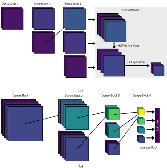
no longer needed to be relearned. Figure 2.7 illustrates the principle behind a DenseNet! ( DenseNet! ). A new parameter for dense nets is the growth rate k, i.e. the number of layers that is added with each dense convolutional layer, that depends on the network architecture and does not change during training.

Each dense block consists out of multiple dense convolution layers that each dense convolution layer adds k layers, which are concatenated to the ”collective knowledge” and therefore preserved. The convolution operations in a dense layer consist of two individual convolution operations. The first convolution operation is the ”bottleneck layer” that increases or reduces the number of feature maps to 4 · k feature maps in a 1 × 1 convolution operation followed by the second convolution operation that reduces the number feature maps to k in a 3 × 3 convolution. The spatial size inside a dense block remains constant and does not change due to added padding.

After each dense block the number of filters is reduced by the compression factor θ, which is set to 0.5 in the example by Huang et al. (2018). This compression is done by a 1 × 1 convolution operations. The spatial size of the image is reduced by half its size by average pooling or 2 × 2 convolution operations with stride 2.

After the final dense block, a final average pooling step is done over the whole image with a single output value for each feature map. In the classification case, a softmax is finally applied over the 1 dimensional output of the of the pooling operation.

Batchnorm

During the training of a neural network, a problem can arise in which the weights

and biases explode and increase uncontrolled. This can cause the network to

fail and produce nonsensical output like infinity or nan (not a number). This

can be caused for example by unnormalized data, too large optimization steps

(a)

(b)

Figure 2.7: Illustration of a DenseNet . Figure a) shows the structure of a dense block. Each dense layer concatenates k new feature maps channel-wise to the

”total knowledge” while maintaining the spatial size of the image. In the final step of the dense block, the data is transformed to half the amount of feature maps with a 1 × 1 convolution and half the spatial size by a 3 × 3 convolution with stride 2. Figure b) illustrates the basic structure of a dense net. The output of each dense net is part of the ”total knowledge”. Each block therefore gets the output of each previous layer as input. After the last dense block, an average pool which outputs a single number is applied over each feature map.

Finally, a softmax function is applied.

2.3. Neural Network Tasks

or wrong weight initializations.

During the training of the network, the network parameters change and therefore the distribution of network activations also changes. This Internal Covariate Shift increases with depth of the network, as each change in distribution is per- petuated through the layers and can increase with each layer. By applying a normalization between the layers instead of just on the input layer, the covari- ance shift can be reduced and the training therefore be stabilized. Batchnorm, as defined by Ioffe et al. 2015, does this on a mini batch level. It calculates the mean and standard deviation of the mini batch and then substracts the mean and divides by the standard deviation. Another side effect of batchnorm is the reduction of overfitting due to its introduction of noise in the activations of each layer.

2.3 Neural Network Tasks

There are many possible tasks that neural networks can help solve. Besides the networks used for the three important tasks in this thesis: classification, regres- sion and autoencoding, there are for example Generative Adversarial Networks, that can create images of realistic faces in StyleGAN by Karras et al. (2018) or Recurrent Neural Networks ( RNNs ) often used in translation tasks or speech recognition tasks.

2.3.1 Classification

Classification is the task of predicting the class that a data point belongs to in a set of k classes. It maps the inputs x to the discrete outputs y, where each output neuron belongs to a class by learning a function f : R ⁿ → {1, ..., k}. On the last layer, a function like the softmax function is applied, that normalizes the output values of all neurons in the output layer together so that the output layer becomes a probability distribution that describes the probability of each input object of belonging to each class. The input object is then assigned the class with the highest value of all classification classes, that is above a threshold value ζ. An example for a classification task is image recognition, where each image is assigned to the corresponding class that can be seen on the image or identify whether an e-mail is spam or not.

2.3.2 Regression

In a regression task, the Machine Learning ( ML ) algorithm learns a relation

between the input and the continuous numerical valued output as the function

f : R ⁿ → R ^m , where m can be 1 for the regression of a single, continuous value or

greater than 1 for the regression of more than one continuous values. Although

(a) (b)

Figure 2.8: Image (a) shows basic image colorization with an autoencoder by Zhang et al. (2016). The right image is the result of the colorization autoencoder of the left image, an image that only exists in black and white. Image (b) shows denoising done by Bigdeli et al. (2017) on an image. The lower left image shows the zoomed in area before the denoizing, the right shows the zoomed in area after denoizing.

this task has a different output format, it is similar to the classification. For instance, a regression task could be the prediction of an object location in an image or the prediction of house prices in an area.

2.3.3 Autoencoder

Autoencoder learn to project the data from a higher dimensional space to a lower dimensional latent space using non linear, learned transformations and then projects it back to the higher dimensional space. In other words, it encodes the input in a learned way and decodes it again. Due to the reduced dimensionality of the intermediate layers, this compression does not work lossless in most cases, as not all information can be propagated through the compression steps.

Often, the input for the Autoencoder is the same as the output and its purpose

is the dimensionality reduction of the data, e.g. it learns to compress and de-

compress an image, but it can also be used to change the output image, like

image denoising, image colorization or anomaly detection, where it is trained

to precisely reconstruct the features of the data, but when applied on anoma-

lies it should fail to reconstruct the data correctly. Examples of Autoencoder

applications can be seen in figure 2.8.

3 Machine Learning in MAGIC

3.1 Current MAGIC Analysis Chain

The current analysis chain in MAGIC is done with the dedicated MAGIC Anal- ysis and Reconstruction Software ( MARS ). MARS consists of multiple different sub-programs, uses CERN’s Root framework (Brun et al. 1996) and is written in C++. In the first step of MARS, the sub-program Sorcerer calibrates the raw data, which contains a waveform for each pixel. Sorcerer reconstructs the pulse shape for each pixel and gathers the intensity and timing information of the pulse. The pulse intensity is then converted to photo electrons generated by the event. This calculation is based on dedicated calibration runs and pedestal events. After the calibration, the images are cleaned using one of mutliple possi- ble cleaning algorithms to remove the background and noise of the image. This is done by the sub-program star. It also calculates the images’ Hillas parameters and more MAGIC specific parameters used for the analysis. Next, the program quate applies cuts to remove images that were not triggered by extensive air showers but due to hardware problems or environmental influences. In the next step, the sub-program superstar is used, which identifies pairs of mono images and combines them to stereo images. Then it calculates parameters that de- pend on the stereo images like impact point or incoming direction. By now, the images still contain images of Extensive Air Shower ( EAS ) caused by γ-photons and hadrons as initial particles. To separate the (hadronic) background events and to select the γ signal events, a Random Forest ( RF ) is used. A random forest is a supervised machine learning algorithm, that is based on numerous decision trees. The decision trees are trained on training data and learn some dependence of the output on the input. Multiple decision trees are used in this case, because a decision tree is prone to overfitting. In the inference, the output of all decisison trees is then averaged and the random forest decides which class it belongs to. Before the RF is used in MAGIC, it is trained using simulated Monte Carlo ( MC ) γ-signal events and off data by the sub-program coach. The RF is applied on the extracted Hillas parameters. This trained random forest is then applied on the source data and another MC data set in the sub-program melibea. This extra MC data set is needed for the γ-ray flux estimation with flute. Currently, the CTAPipe package under development, a completely new

IACT analysis software written in python, which will be used for data analysis

in CTA but is also adjusted to work with magic data as CTAPipe-mpp.

Figure 3.1: Hillas parameters’ geometrical definition for an ellipse fitted onto a shower image with a source position of the initial particle that caused the shower at X.

3.2 Hillas Parameters and Particle Parameter Reconstruction

To get parameter of the shower and the initial particle, Hillas 1985 introduced the hillas parameters; a way of parametrizing the images of IACT by fitting an ellipse to the shower image as shown in shown in Figure 3.1 and extracting the following parameters:

• W Width of the ellipse

• L Length of the ellipse

• d Nominal angular distance between the images’ center of gravity and the source position in the camera frame

• φ Angle between the images’ main axis and the images x-axis

• ψ Angle of the ellipses’ orientation

• Size Total amplitude of the image

• Position Position of the ellipses’ center in camera coordiantes

Furthermore a timing parameter is calculated of the impact times of the Cherenkov

photons in the camera. In the analysis, the absolute value of the timing param-

eter is used due to the ambiguity of the direction of the timing caused by the

3.2. Hillas Parameters and Particle Parameter Reconstruction

Figure 3.2: Illustration of a stereo position reconstruction in IACTs by Fruck (2015)

charged particles moving faster than the speed of light in the air. The origin of a shower can be reconstructed with these parameters as point along the ellipses’

long axis with a distance disp away from the ellipses’ center. With just one tele- scope, the direction of the shower is ambiguous, because the shower origin could be located at both sides of the image. With at least two telescopes, operated together in stereo mode, the interception point of the combined shower images’

reconstructed directions allows for unique reconstruction of the particles’ origin direction. An improved method for the origin reconstruction is the usage of a random forest algorithm that calculates the disp of both images based on the hillas parameters as input. This disp results in two points for each image along its ellipses’ long axis. The weighted mean of the two points that are closer together is the reconstructed origin of the shower. Figure 3.2 illustrates the principle of the direction reconstruction.

The distance between the reconstructed origin position and the position of the

observed source Θ is used in the analysis to exclude background events. Figure

3.3 shows a Θ ² plot that is used for rejection of background events. The excess

events at low Θ ² are considered to be signal events by source pointed at. The

Θ ² plot shows the squared angular distance between the reconstructed origin of

the shower and the expected source position in the camera. All other events are

Figure 3.3: Examplary Θ ² plot from the Crab Nebula by Aleksi´ c et al. (2012)

excluded as background events. Furthermore, the impact parameter, i.e. the point where the shower axis intercepts the plane constructed by the telescopes’

base, and the height of the shower maximum can be calculated with the stereo parameters.

The hillas parameters described above are then used to reconstruct the direc- tion and energy of the initial particle as well as separate the γ events from the background events. While the background rejection with the current analysis methods works well in the high energy regime of more than 1 TeV, the back- ground rejection at low energies is still not very good. In the same way, the reconstruction of the direction and energy of the initial particle works better in the high energy than in the low energy regime. Furthermore, the parametriza- tion of the images reduces the information we can get from the image. Therefore a method that utilizes all the pixel and timing information could produce better results.

3.3 MAGIC Monte Carlo Simulations

The first step in the MC simulations for MAGIC is the simulation of the ex-

tensive air shower and its emitted Cherenkov photons using the Cosmic Ray

Simulations for Kascade ( CORSIKA ) package. The CORSIKA program creates

detailed simulations of extensive air showers caused by particles hitting the

atmosphere by tracking the initial and created particles and simulating their in-

teractions with other particles as well as their decays and creation of secondary

particles like Cherenkov photons and neutrinos. For MAGIC simulations, the

3.3. MAGIC Monte Carlo Simulations

(a) (b)

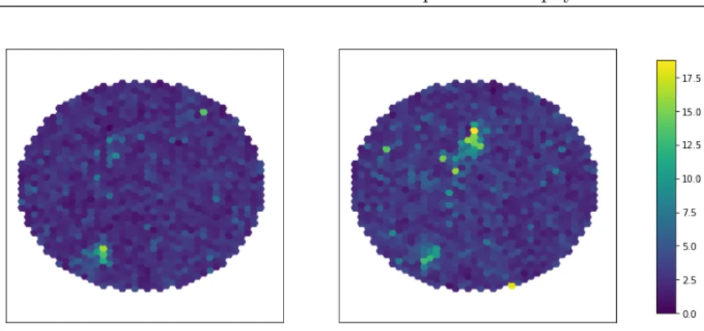
Figure 3.4: Images of two different γ-event showers simulated with the MAGIC simulation chain, calibrated with Sorcerer. a) shows a noiseless image and b) shows an image with noise added in camera.

Cherenkov photons’ coordinates and directions at the moment of production are saved in the output file, which is then input into the reflector program, which simulates the Cherenkov photons from their creation to the camera, taking into account the atmospheres’ absorption, scattering etc. and the telescopes’ optical properties but without the response of the camera. Next, the program cam- era is used to simulate the response of the MAGIC cameras and usually adds simulated electronic noise and background. The MC images can now be put into the data analysis chain as described above like the real data events. Figure 3.4 shows (a) a calibrated simulated shower image without any noise and (b) a calibrated simulated shower image with simulated noise. The noise added in the camera program is sufficiently comparable to the real noise for the current anal- ysis chain. Nevertheless, more sophisticated algorithms can learn the difference between the images containing simulated noise and data.

While the development of electromagnetic air showers is well known, the de-

velopment of hadronic air showers is still not perfectly clear. A lot of inter-

action and decay cross-sections of the intermediate particles, especially due to

the strong interactions and at very high energies, because collider experiments

cannot reach such high energies yet. This introduces some uncertainty in the

production of proton simulations. Furthermore, the development of hadronic

air showers is complicated and takes a long time to simulate compared to elec-

tromagnetic showers caused by γ-rays. Therefore, proton simulations are rather

uncommon in MAGIC and most of the time off-data is used as background data,

as in most cases the initial properties of the cosmic rays are not relevant.

Figure 3.5: Example of pixels covered by a square convolution (top) and by a hexagonal convolution (bottom) applied on a hexagonal grid. It can be seen that the square convolution covers more pixels than the direct neighbours and violates the symmetry of the grid. The hexagonal convolution corresponds to the grid and only covers the neighbours. Image by Steppa et al. (2019)

3.4 Neural Networks

HexagDLy

All current major machine learning frameworks like Tensorflow and PyTorch only feature convolution operations on square grids designed for square pixels, as they are used in everyday applications like digital images. In science however, hexagonal grids are more prominent due to their better approximation round shapes as well as induction of more spatial symmetries and subdivision of an area without gaps, while keeping the borders between pixels as short as short possible. Applying the square convolutions on hexagonally sampled data ignores the neighbour relations between pixels as shown in figure 3.5 and violates the symmetry of the data.

As the MAGIC telescopes’ cameras also feature hexagonal pixels, a solution to handling this hexagonally sampled data has to be found. Several studies were conducted on resampling the data to be represented by a square grid like over- sampling, where each hexagonal pixel is approximated by 4 or more square pixels or linear interpolation. Although they show good performance in some cases, it is shown by Steppa et al. (2019) that using special hexagonal convolution al- gorithms improve the performance, stability and convergence during training of the CNN. The implementation of a hexagonal convolution algorithm was done by Steppa et al. (2019) for PyTorch in a library called hexagDLy. It works by applying multiple, differently spaced convolutions on the padded, hexagonally sampled data, mapped to a square grid as shown in figure 3.6.

Although the performance of HexagDLy is worse than normal convolutions,

3.4. Neural Networks

Figure 3.6: Individual steps for hexagonal convolution done by hexagDLy on an examplary hexagonal grid. The different convolutions with different kernels, paddings and strides are executed on the grid and then merged and added together to result the convoluted hexagonal grid. Image by Steppa et al. (2019)

the consideration of hexagonal convolutions and therefore the use of hexagonal convolutions could be worth it. For the following investigations, the PyTorch open source machine learning library was used because of its state of the art technology, active development and the availability of the hexagonal convolution library HexagDLy.

3.4.1 Data Loading

For the usage of the event images in the machine learning algorithms, the

MAGIC data calibrated with Sorcerer does not undergo the data analysis chain

but is loaded with the CTAPipe-mpp framework. The images in the output files

from sorcerer are saved as photo electrons per pixel as well as peak position in

time in a spiral structure, starting at the central pixel and moving outwards

clockwise. First a function had to be developed to transform the spiral data

into a square grid, which can then be used by HexagDLy. By simply moving

every second row of the square grid up by half a unit, the grid can be plotted as

hexagonal. The data contains the photo electrons and peak times per pixel as

well as the pointing direction of the telescopes and, in the case of Monte Carlo

simulations, the information of the simulation: initial particle id and energy, the

azimuth and altitude of the particles’ origin, the height of its first interaction

in the atmosphere as well as the impact parameters core x and core y of the

shower. The origin coordinates of the particle are transformed to a telescope

frame, where the coordinate system aligns with the optical axis of the telescopes

and the horizon and to the camera frame, where the location is saved as x and