Food Prices, Wages, and Welfare in Rural India

Policy Research Working Paper 6412

Food Prices, Wages, and Welfare in Rural India

Hanan G. Jacoby

The World Bank

Development Research Group

Agriculture and Rural Development Team April 2013

WPS6412

Public Disclosure Authorized Public Disclosure Authorized Public Disclosure Authorized Public Disclosure Authorized

Abstract

The Policy Research Working Paper Series disseminates the findings of work in progress to encourage the exchange of ideas about development issues. An objective of the series is to get the findings out quickly, even if the presentations are less than fully polished. The papers carry the names of the authors and should be cited accordingly. The findings, interpretations, and conclusions expressed in this paper are entirely those of the authors. They do not necessarily represent the views of the International Bank for Reconstruction and Development/World Bank and its affiliated organizations, or those of the Executive Directors of the World Bank or the governments they represent.

Policy Research Working Paper 6412

This paper considers the welfare and distributional consequences of higher relative food prices in rural India through the lens of a specific-factors, general equilibrium, trade model applied at the district level. The evidence shows that nominal wages for manual labor both within and outside agriculture respond elastically to increases in producer prices; that is, wages rose faster in rural districts growing more of those crops with large price run-ups over 2004–09. Accounting for such wage gains, the analysis finds that rural households across the income spectrum

This paper is a product of the Agriculture and Rural Development Team, Development Research Group. It is part of a larger effort by the World Bank to provide open access to its research and make a contribution to development policy discussions around the world. Policy Research Working Papers are also posted on the Web at http://econ.worldbank.org.

The author may be contacted at hjacoby@worldbank.org.

benefit from higher agricultural commodity prices.

Indeed, rural wage adjustment appears to play a much

greater role in protecting the welfare of the poor than the

Public Distribution System, India’s giant food-rationing

scheme. Moreover, policies, like agricultural export bans,

which insulate producers (as well as consumers) from

international price increases, are particularly harmful to

the poor of rural India. Conventional welfare analyses

that assume fixed wages and focus on households’ net

sales position lead to radically different conclusions.

Food Prices, Wages, and Welfare in Rural India

Hanan G. Jacoby ^∗

Keywords: Agriculture, Trade, Specific-factors Model, General Equilibrium JEL codes: Q17, Q18, F14

Sector Board: POV

∗

Agriculture and Rural Development Unit, Development Research Group, The World Bank. E-mail:

hjacoby@worldbank.org. I am grateful to David Atkin, Madhur Gautam, Denis Medvedev, Rinku Murgai,

Maros Ivanic, Will Martin, and Vinaya Swaroop for useful suggestions and to Maria Mini Jos for assistance

in processing the data. The findings, interpretations, and conclusions of this paper are mine and should not

be attributed to the World Bank or its member countries.

1 Introduction

Elevated food prices over the last half decade have provoked a rash of government interven- tions in agricultural markets across the globe, often in the name of protecting the poor. Of course, it is well recognized that many poor households in developing countries, especially in rural areas, are also food producers and hence net beneficiaries of higher prices. ¹ Even so, there is another price-shock transmission channel, potentially more important to the poor, that has received far less attention in the literature: rural wages. ² To what extent do higher agricultural commodity prices translate into higher wages? For rural India, home to roughly a quarter of the world’s poor (those living on less than $1.25/day), the answer to this question can have momentous ramifications. After all, the vast majority of India’s rural population relies on the earnings from their manual labor, most of which is devoted to agriculture. ³ Any thorough accounting of the global poverty impacts of improved terms of trade for agriculture must, therefore, confront rural wage responses in India.

Aside from direct income effects for consumers and producers, as in the textbook partial equilibrium analysis (e.g., Singh, Squire, Strauss, 1986, Deaton, 1989), higher agricultural prices, in principle, induce three types of indirect, or general equilibrium, effects concomitant with higher wages: (1) higher labor income; (2) lower capital (land) income due to higher labor costs; (3) higher prices for nontradables. To account for these channels in a manner that is both theoretically coherent and transparent, I integrate a standard three-sector, specific factors, general equilibrium model of wage determination (Jones, 1971,1975) into an otherwise conventional (first-order) household welfare change calculation. ⁴ I use this

1

Ivanic et al. (2012), Wodon et al., (2008), and World Bank (2010a) provide recent multi-country assess- ments of the the welfare impacts of food price increases accounting for such producer gains.

2

Ravallion (1990) surveys the debate in development on the nexus between the intersectoral terms of trade and poverty. Shah and Stiglitz (1987) provide an early theoretical treatment. In their cross-country study, Ivanic and Martin (2008) incorporate price-induced changes in wages for unskilled labor derived from nation-level versions of the GTAP computable general equilibrium model.

3

Indeed, rising wages are seen as the major driver of rural poverty reduction in recent decades (Datt and Ravallion, 1998; Eswaran, et al. 2008; Lanjouw and Murgai, 2009).

4

Porto (2006) (and subsequently Marchand, 2012) comes closest to my approach in the context of trade

liberalization, but differs in some important details. Primarily, he keeps the general equilibrium model, in

his case applied to the country as a whole, in the background of the analysis.

generalization of Deaton (1989) to examine the distributional impacts of higher agricultural prices in rural India.

Appealing to the widely noted geographical immobility of labor across rural India, ⁵ I apply the specific factors model at the district level, treating each of these administrative units for theoretical purposes as a separate country with its own labor force but with open commodity trade across its borders. ⁶ Thus, I allow that the elasticity of the rural wage with respect to an index of agricultural prices is not a single number for India as a whole, but varies with the structure of the particular (district) labor market. Moreover, under certain assumptions on the technology and preferences, I obtain a readily interpretable closed-form solution for this elasticity as a function of parameters that I can easily calculate from micro- data.

My empirical analysis shows that nominal wages for manual labor across rural India respond elastically to higher agricultural prices. In particular, wages rose faster in the districts growing relatively more of the crops that experienced comparatively large run-ups in price over the 2004-5 to 2009-10 period. Moreover, the magnitude of these wage responses is broadly consistent with a specific-factors model in which labor is perfectly mobile across production sectors. Indeed, I also explore a version of the theoretical model in which labor markets are segmented so that workers cannot shift from agriculture to the services or manufacturing sectors. This alternative labor market assumption turns out to have significantly different welfare implications in the Indian context than the unsegmented case.

Fortunately, it has different empirical implications as well: Under labor market segmentation, nonagricultural wages (for manual labor) respond to changes in agricultural prices with a

5

See, e.g., Topalova (2007, 2010), Munshi and Rosenzweig (2009), and World Bank (2010b). Kovak (2011) applies a specific-factors model to sub-national units in Brazil, a country with much greater geographical labor mobility than India. Despite incorporating cross-regional labor migration over an entire decade into his empirical strategy, it turns out not to matter for local wage responses to trade reform.

6

In this framework, capital (land, in agriculture) is also assumed immobile across both districts and

production sectors. Mussa (1974) was perhaps the first to argue that the Stolper-Samuelson theory, with

its assumption of perfect factor mobility, is inadequate for analyzing the relevant distributional effects of

commercial policy. This is true a fortiori in the context of food price “crises”, where long-run welfare

considerations play virtually no role in the policy debate.

relatively low elasticity, as intersectoral spillovers are muted, if not nugatory. The evidence, however, is inconsistent with this strong form of segmentation.

Existing studies of the relationship between agricultural commodity prices and rural wages are based on aggregate time series data from countries that were effectively autarkic in the main food staple (pre-1980s Bangladesh in Boyce and Ravallion, 1991, and Rashid, 2002; the Philippines in Lasco et al., 2008), thus raising serious endogeneity concerns. A closely related and much larger literature based on micro-data considers the labor market effects of trade liberalization (see Goldberg and Pavcnik, 2007, for a review). ⁷ My estimation strategy follows the “differential exposure approach” employed in studies of the local wage impacts of tariff reform (most recently in Topalova, 2010, McCaig, 2011, and Kovak, 2011).

Instead of considering the interaction between changes in industry protection rates and local industry composition (as in these papers), I exploit the huge variation across Indian districts in the crop composition of agricultural production coupled with differences in the magnitude of wholesale price changes across crops. Of course, price changes observed in local domestic markets cannot be treated as exogenous and must be instrumented for.

In rural India, the elastic rural wage response to changes in agriculture’s terms of trade has striking distributional implications. Higher food prices, rather than reducing the welfare of the rural poor as indicated by the conventional approach, which ignores wage impacts, would actually benefit both rich and poor alike, even though the latter are typically not net sellers of food. ⁸

In the next section, I sketch the theoretical framework and develop my empirical testing strategy. Section 3 discusses the econometric issues and the estimates. Section 4 derives and implements the welfare elasticity formulae, paying particular attention to the role of India’s vast Public Distribution System, which rations food staples to the poor. The price-

7

Topolava (2010) and Marchand (2012), among others, consider the reduced-form wage and poverty impacts of India’s broad-based trade liberalization of the 1990s. However, these studies do not isolate the effects of a change in the relative price of food.

8

To be sure, the increase in rural wages may lag the increase in consumer prices, and so the conventional

analysis may be more appropriate for the very short run. This paper does not speak to the timing issue.

shock buffering impact of this program provides a useful comparator to that of rural wage adjustment in general equilibrium. I conclude, in section 5, with a discussion of the Govern- ment of India’s responses to the 2007-08 food price spike, notably its export ban on major foodgrains.

2 Framework

2.1 A general equilibrium model

Consider each district as a separate economy with three sectors: agriculture (A) and man- ufacturing (M), both of which produce tradable goods, and services (S), which produces a nontradable. Output Y _i in each sector i = A, M, S is produced with a specific (i.e., immobile) type of capital K _i , along with manual labor L _i and a tradable intermediate input I _i . In the case of agriculture, K _A is in fact land and I _A is, e.g., fertilizer. Manual labor is perfectly mobile across sectors but its supply is fixed at L = L A + L M + L S within each district (later, I reconsider the first of these assumptions). Nonmanual labor is assumed to be exogenously fixed for simplicity. ⁹

To deal with multiple crop outputs Y ₁ , ..., Y _c , let Y _A = G(Y ₁ , ..., Y _c ), where the product transformation function G is assumed to be homogeneous of degree one. A price index P _A thus exists such that P _A Y _A = P c

j=1 P _j Y _j , which upon differentiation yields

P b A = X

j

s j P b j (1)

where “hats”denote proportional changes and s _j is the value share of crop j.

Now let W be the nominal wage for manual labor and P _M and P _S be the prices of manufactures and services, treating the former output price as fixed so that manufactures

9

In rural India, as we will see, nonmanual labor accounts for only 17 percent of employment days, though

a considerably larger portion of household income. The exogeneity assumption can be motivated by thinking

about nonmanual labor as requiring a higher level of education, which cannot be obtained in the short-run.

is the numeraire. Similarly, I take the price of all intermediate inputs as fixed. Finally, let Π _A be the average return on land. ¹⁰ Given that farmers are price-takers in all markets, we have (from price equals unit cost)

α _L c W + α _K Π b _A = P b _A (2) where, under constant returns to scale, the input cost shares in agriculture, the α _l , l = K, L, I, are such that α _K + α _L + α _I = 1. Similar equations hold for the other sectors, each with its own set of input cost shares (see Appendix A.1 for technical details). In the interest of clarity and because it will make no appreciable difference empirically (see below), I assume equal input cost shares across sectors in the sequel.

The implied elasticity of the wage for manual labor with respect to the agricultural price index, W / c P b _A , is given by

ψ = β A + δβ S

α _L + α _K (3)

where the β _i = L _i /L are the sectoral labor shares and δ = P b _S / P b _A . Combining (2) and (3) also gives

Π b _A / P b _A = 1 α K

(1 − α _L ψ) . (4)

So the elasticity of the return on land with respect to the agricultural price index incorpo- rates the direct (positive) effect of price changes on producer profits as well as the indirect (negative) effect of price induced wage changes.

As for the intuition underlying equation (3), in the special case α _I = β _S = 0 it is extremely simple: As food prices increase, the marginal value product of labor rises in agriculture, drawing labor into farm-work from the other sectors (in this case, only manufacturing) until equality of marginal value products across sectors is restored. The larger agriculture is in

10

That is, for production function F

, total return or profit is Π

K

= P

F

(L

, I

, K

) −P

I

−W L

.

relation to nonagriculture, the greater has to be the exodus of labor from the latter sector in proportional terms, the greater has to be the consequent rise in the value of the marginal product of labor, and the greater, therefore, has to be the rise in the rural wage. Given the Cobb-Douglas assumption, ¹¹ the wage elasticity exactly equals the relative size of the agricultural sector, or β _A . If α _I > 0, then the wage-price elasticity exceeds β _A . The source of this amplification effect is the increase in intermediate input use induced by higher agricultural prices, which boosts the marginal product of labor in agriculture and pulls even more labor out of the other sectors.

The dependence of the wage-price elasticity on β _S , in the more general case, has to do with the endogeneity of the output price in the nontraded sector. A rise in the wage induced by higher agricultural prices reduces the supply of services; it also can increase the demand for services due to an income effect. Both forces put upward pressure on the price of services, which reverses the aforementioned outflow of labor from that sector into agriculture. Thus, the larger the service sector, the greater has to be manufacturing’s relative contribution to the shift of labor into agriculture and, hence, the greater has to be the resulting rise in the rural wage.

For given β _S , the wage-price elasticity is also increasing in δ, the elasticity of the service sector price with respect to the agricultural sector price. In general, δ depends on the price and income elasticity of demand for services as well as on the response of aggregate income y to increases in the agricultural price. In particular, I will assume that y consists of the total return on land, manual labor earnings, and exogenous earnings, E, from nonmanual labor such that ¹²

y = Π _A K _A + W L + E. (5)

11

See Appendix A.1. Although more general results can be derived using CES production functions (as in Kovak, 2011), empirical implementation would require information on elasticities of factor substitution.

12

Neither the returns to capital in manufacturing nor in services are assumed to accrue to rural households.

While ultimately for empirical convenience, this simplification is likely to be fairly innocuous.

Appendix A.1 derives an explicit expression for δ in terms of the α _l , β _j , and the income component shares for the case of a unitary-elastic demand for services (Cobb-Douglas pref- erences).

One might, however, question the assumption that the demand for services responds substantially to income changes over the five-year time-frame of my empirical analysis. That is, stepping outside of the static model now, it may take some time before households behave as if changes in income induced by agricultural price innovations are permanent. Under this view, income effects on the demand for services can be zeroed out in solving for the wage- price elasticity (see Appendix A.2). I denote this elasticity by ψ ^SR to indicate its validity (grosso modo) in the short-run wherein price-induced income changes are taken as transitory.

2.2 Segmented labor markets

Thus far I have maintained the assumption that workers can move costlessly between agricul- ture, manufacturing, and services. Intuition suggests that restricted intersectoral mobility of labor would limit spillover effects from changing agricultural prices, concentrating wage gains within agriculture. To be precise, suppose that mobility costs are sufficiently high that labor is effectively fixed in agriculture, though still mobile between manufacturing and ser- vices. Agriculture and nonagriculture now each have a unique equilibrium wage. As I show in Appendix A.3, the wage-price elasticity in agriculture is 1/(α _L +α _K ) and in nonagriculture is

ϕ = δ ⁰ β _S ⁰

α _L + α _K (6)

where δ ⁰ = P b _S / P b _A and β _S ⁰ = L _S /(L _S + L _M ) (note that, in general, δ ⁰ 6= δ and β _S ⁰ > β _S ).

The key point here is that the magnitude of the intersectoral price spillover, reflected in the

elasticity ϕ, depends entirely on the structure of demand for services. How much manual

labor is drawn back into the service sector to accommodate the production increase induced

by higher demand is directly related to β _S ⁰ , the size of this sector relative to nonagriculture as a whole.

If the demand for services is unresponsive to changes in income induced by higher agri- cultural prices, as I have suggested might be the case in the short-run, then the segmented model delivers a very sharp prediction. In this case, δ ⁰ = 0 and, consequently, ϕ ^SR = 0.

In other words, until (permanent) income effects kick in, there are zero inter-sectoral price spillover effects in a segmented economy.

2.3 A taxonomy of wage-price elasticities

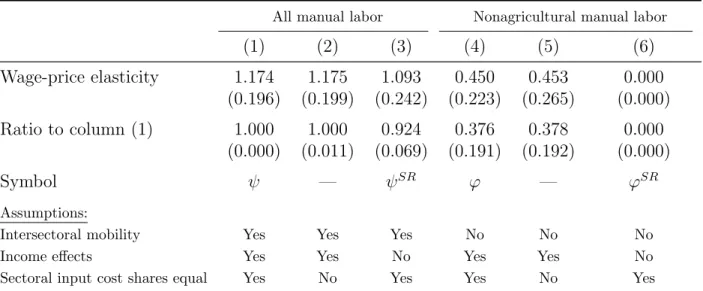
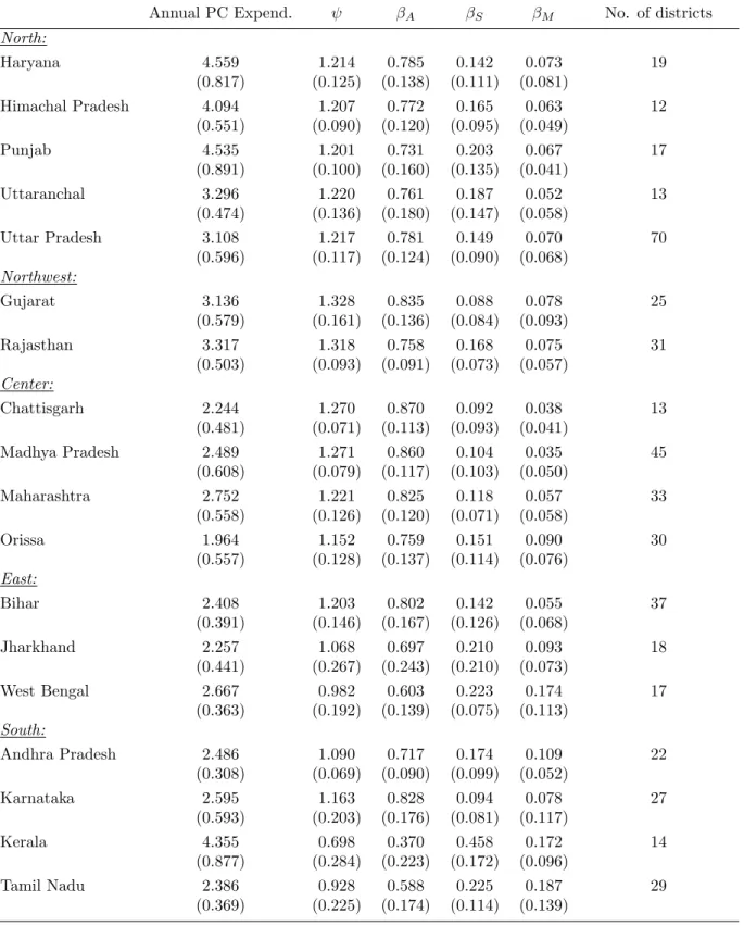
The theoretical framework yields wage-price elasticities as functions of input cost shares, sectoral labor shares, and other parameters, all of which can be estimated from nationally representative data collected by India’s National Sample Survey (NSS) Organization (see Appendix B for details). Table 1 summarizes the results of these calculations for 472 districts in 18 geographically contiguous states of India, containing the vast bulk of its rural population. ¹³

Columns 1-3 present wage-price elasticities implied by perfect sectoral mobility and columns 4-6 the nonagricultural wage-price elasticities implied by labor market segmen- tation. Thus, in column 1, the ψ from my baseline model, which assumes a unitary elastic demand for services and equal input cost shares across sectors, averages 1.17 across dis- tricts. ¹⁴ Such high elasticities reflect large values of β _A ; for the average rural district, around three-quarters of manual labor days (adjusted for efficiency units; see Appendix B.2) are spent in agriculture. Statewise statistics on labor shares, per-capita expenditures, and ψ are reported in Appendix Table C.1.

13

Excluded are the peripheral states of Jammu/Kashmir in the far north and Assam and its smaller neighbors to the north and east of Bangladesh. Included states, organized into five regions, are North:

Harayana, Himachal Pradesh, Punjab, Uttar Pradesh, and Uttaranchal; Northwest: Gujarat and Rajastan;

Center : Chhattisgarh, Madhya Pradesh, Maharashtra, and Orissa; East: Bihar, Jharkhand, and West Bengal; South: Andhra Pradesh, Karnataka, Kerala, and Tamil Nadu. See Appendix Table C.1.

14

By contrast, the smattering of aggregate time-series evidence that exists for other countries suggests a

wage-food price elasticity somewhat less than unity (see Lasco et al., 2008, for a review).

While it is straightforward to allow for sector-specific input cost shares using the results in Appendix A.1, it hardly matters. Cost shares of value-added for Indian manufacturing and service sectors based on national accounts are available from Narayan et al. (2012).

As seen in column 2, however, they yield virtually identical elasticity results as in the equal shares case. While the labor cost share in manufacturing is, to be sure, much lower than that in agriculture (and in services), so is the capital share. Hence, the ratio of capital to labor shares, which is most relevant to the calculations, is actually quite similar across sectors.

The third column of Table 1 reports wage-price elasticities ignoring income effects on the demand for services. As argued earlier, ψ ^SR may provide the more realistic wage response over relatively short horizons, such as the five-year period of my empirical analysis. Intu- itively, suppressing income effects dampens the rise in the price of services that accompanies higher agricultural prices. As a consequence, less labor needs to be diverted to the service sector, so the rural wage does not have to rise as much. In the event, ψ ^SR is 92 percent as large, on average, as the baseline ψ.

In the remainder of Table 1, we see (col. 4) that segmented labor markets, under otherwise identical assumptions, deliver a much smaller wage-price elasticity than the baseline model. ¹⁵ The average value of ϕ across districts is only 0.45, again barely changing when the equal cost shares assumption is relaxed (col. 5). For completeness, column 6 notes that ϕ ^SR = 0. To reiterate, if the income effect on the demand for nontradables is inoperative and labor markets are segmented, then non-agricultural wages are completely unresponsive to agricultural price changes.

2.4 Testing the theory

We have just seen that the wage-price elasticity, c W / P b _A = ψ, is not a single number for all of India, but rather varies by district according to, among other factors, the sectoral labor

15

Recall that what matters in the calculation of ϕ is the importance of services relative to nonagricultural

manual labor (services + manufacturing). This services share, β

, averages 0.67 across the 464 districts

with any nonagricultural manual labor (based on NSS64; see Appendix B.2).

shares. In principle, one could estimate a separate ψ for each district, or perhaps for each type of labor market, and compare the results to the ψ implied by the theory as summarized in Table 1. In practice, however, this would require long time-series of wages and prices for each district, which are unavailable. Nevertheless, I can do the next best thing by estimating the regression analog to W /ψ c = P b _A , or

∆w d /ψ d = c + γ X

j

s d,j ∆p j + ε d (7)

where c is an intercept, γ is a slope parameter, and ε d is a disturbance term for each district d. ¹⁶ Under the null hypothesis γ = 1, the theory, along with its auxiliary assumptions, can be said to hold true on average. Note that equation (7) simply replaces proportional changes c W and P b _A (cf., equation (1)) by their respective empirical counterparts. Thus, ∆w _d is the difference in log wages between years t − k and t and the ∆p _j are the corresponding time-differences in log prices of crop j. Which prices to use and the econometric issues that arise from this choice are the main topic of Section 3.4.

Turning to segmented labor markets and to wages in the nonagricultural sector (N A), we may write W c _{N A} /ψ = γ P b _A , modifying the left-hand side of equation (7) accordingly. In this case, γ reflects the degree of intersectoral labor mobility. Under the null of perfect mobility, ¹⁷ γ = 1, which says that the price elasticity of nonagricultural wages, ϕ, is equivalent to the price elasticity of wages in general, ψ. By contrast, under the segmented labor market alternative, c W _{N A} /ϕ = P b _A , which is to say that γ = ϕ/ψ. Notice that the power of my test of γ = 1 against this alternative depends on how far ϕ/ψ deviates from unity, larger deviations being easier to detect in finite samples. In this regard, Table 1 provides some cause for optimism; φ/ψ averages only 0.376 under unitary-elastic demand for services and

16

An alternative to equation (7) would leave ψ

on the right-hand side and estimate γ off of the interaction between ψ

and the price change variable. The downside of this approach is that, insofar as ψ

is not perfectly measured, it introduces an errors-in-variables problem.

17

More precisely, this is the joint null that intersectoral labor mobility is perfect and that the model is

true (on average).

may be as small as zero if income effects are negligible in the short-run (i.e., φ ^SR /ψ ^SR = 0). ¹⁸

3 Empirical Analysis

3.1 Domestic agricultural markets

Since at least the 1960s, Indian governments, both at the national and state level, have intervened extensively in agricultural markets. Interstate trade in foodstuffs is often severely circumscribed through tariffs, taxes and licensing requirements (see Atkin, 2011, for a review) with some states (e.g., Andhra Pradesh) going so far recently as to prohibit the exportation of rice to other states (Gulati, 2012). The Government of India also sets minimum support prices (MSPs) at which major food crops are, or at least can be, procured for eventual release into the nationwide public distribution system (PDS). In practice, however, the level of procurement, and thus the extent to which the MSPs are binding, varies greatly by crop and state, and even within states (Parikh and Singh, 2007). The principal foodgrains, rice and wheat, have, in recent years, been the overwhelming focus of government procurement efforts, concentrated in the states of Punjab and Haryana, often for lack of storage capacity and marketing infrastructure elsewhere. By contrast, procurement of pulses and oilseeds has been minimal, as market prices have consistently exceeded MSPs. ¹⁹

During and after the sharp run-up in international food prices in 2007-08, the Government of India imposed export bans on rice, wheat, and a few other agricultural commodities in an attempt to tamp down domestic price increases. Meanwhile, over several consecutive years, MSPs for rice and wheat (and most other major crops) were raised substantially, partly in

18

By contrast, the response of agricultural wages to food price changes would not provide an informative test of perfect intersectoral mobility. In particular, consider W c

/ψ = γ P b

. In the segmented case, W c

/ P b

averages 1.35, which is only 21 percent larger than the baseline ψ in column 1 of Table 1. In other words, γ = ϕ/ψ averages around 1.21 under the segmentation alternative, which is relatively ‘close’ to 1 given the standard errors we will be dealing with in Section 3. Hence, using agricultural wages, the null and alternatives will be practically indistinguishable.

19

See the reports by the Commission for Agricultural Costs and Prices on http://cacp.dacnet.nic.in/ for

more details.

response to international prices; huge stockpiles of foodgrains were subsequently accumulated through government procurement (World Bank, 2010c; Himanshu and Sen, 2011).

The upshot of these interventions is that output prices faced by Indian agricultural pro- ducers do not always perfectly track those in international markets. ²⁰ Moreover, since domestic market integration is somewhat limited (especially in the case of rice), there is con- siderable variability across states in crop price movements. On the one hand, this variation may reflect differential transmission of exogenous price pressure (e.g., because of varying levels of state procurement or exposure to trade, both with other countries and with other states); on the other hand, it may reflect localized supply or demand shocks, which can also drive rural wages directly.

3.2 Crop prices

Wholesale crop price data averaged at the state level from observations at several district markets per state (and weighted by district production), are compiled by the Ministry of Agriculture, as are production and area data at the district level. So as to focus on a period of substantial price movement, as well as to match the NSS wage data (see below), I consider state-level price changes between the 2004-05 and 2009-10 crop marketing seasons. Given the relative ease of moving produce across district (as opposed to state) lines, state-level wholesale prices seem the appropriate measure of farmer production incentives. ²¹

I base the crop value shares, the s d,j in equation (7), on production data from the 2003-04 crop-year, which has the best district/crop coverage for the pre-2004-05 period. Value of production is calculated at 2004-05 state-level prices. Note, however, that I do not take the value-weighted sum of price changes across every single agricultural product grown in India.

Price data for many of the minor field crops and the tree crops are incomplete or not reliable.

20

This is true for the principal intermediate input in agriculture as well. Despite a substantial upsurge in the international prices of chemical fertilizers beginning in 2007, retail prices in India, which are set by the central government, remained uniform and unchanged over the 2004-09 period (Sharma, 2012).

21

Since sugarcane is sold mostly to mills and not in wholesale markets, I use the national MSP or, when

relevant, “State Advised Prices,” which tend to be much higher and, hence, closer to international cane

pricing standards (see Gulati, 2012).

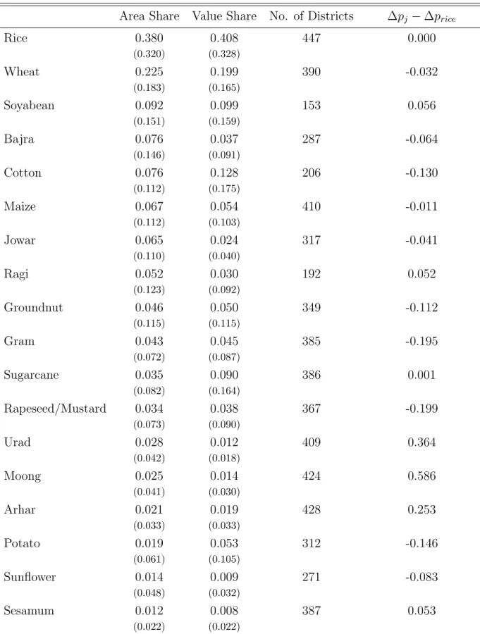
Moreover, the associated production data are often inaccurate (especially for vegetables and tree products). I thus select major field crops according to the criteria that they cover at least 1 percent of total cropped area nationally or that at least 5 districts had no less than 10 percent of their cropped area planted to them in 2003-4. These 18 crops, listed in Table 2 in descending order of planted area, comprise some 92 percent of area devoted to field crops in 2003-04 in the major states of India. ²² Table 2 also reports national average log-price changes (weighted by the state share of total production) relative to rice. Thus, in the first row, the relative price change for rice is zero, quite negative for several important crops (e.g., cotton, gram, groundnut, mustard/rapeseed) and highly positive for pulses (Urad, Moong, and Arhar).

3.3 Wages

Wage data are derived from the NSS Employment-Unemployment Survey (EUS), normally conducted every five years. The most recent round, the 66th, collected in 2009-10, is the first conducted in the wake of the food price “crisis” of 2007-08, whereas the 61st round of 2004-05 most closely preceded it. Once again, in the spirit of the theoretical model, I focus on manual labor, which constitutes nearly 83 percent of days of paid employment in rural areas. ²³ The first-stage of the estimation takes individual log daily wages in the last week and regresses them on district fixed effects as well as a quadratic in age interacted with gender.

Thus, I estimate the respective log-wage district fixed effects, w d,09 and w d,04 , separately for each round, removing, via the constant terms, year effects due to, e.g., general inflation.

22

One could assume that minor crop prices did not change at all over the five-year period in question, though this would still leave the problem of missing base-year minor-crop prices for calculating total crop value shares. At any rate, the zero price change assumption seems untenable prima facie. More appealing is to assume that the average change in minor crop prices is equal to the average change in major crop prices, where averages are weighted by value shares within the respective crop category. Under this assumption, the average of major crop prices weighted by major crop value shares (which is what I observe) is identically equal to the average of all crop prices weighted by total crop value shares (which is what I require).

23

The NSS-EUS categorizes jobs in terms of manual and non-manual labor only for rural, not urban,

workers. Based on the 61st round sample of nearly 39,000 individuals, the population-weighted proportions in

each category are as follows: 58% in manual-agricultural; 24% in manual nonagricultural; 18% in nonmanual

(virtually all in nonagriculture). For the 66th round sample of some 30,000 individuals, the corresponding

proportions are 51%, 30%, and 19%, respectively.

Estimates of the standard errors of the fixed effects σ(w _d,09 ) and σ(w _d,04 ), which I use below to construct regression weights, are obtained following the procedure of Haisken-DeNew and Schmidt (1997).

3.4 Identification

Rewriting equation (7) to reflect the price data discussed above, I wish to estimate

∆w _d /ψ _d = c + γ X

j

s _d,j ∆p _{ST AT E}

_,j + ε _d . (8) where ST AT E _d denotes the state in which district d is located. There are two endogene- ity issues to contend with: measurement error and simultaneity between wage and price changes.

As to the first issue, both the crop value shares, s _d,j , and the crop-specific log-price changes, ∆p _{ST AT E}

_,j , may be measured with error. Putting aside the latter concern mo- mentarily and assuming that measurement error is confined solely to value shares, I could deploy the instrument

IV 1 _d = X

j

a _d,j ∆p _{ST AT E}

_,j (9)

where a _d,j is the area share of crop j in district d. To be sure, cropped areas may also be measured with error, but these errors should not be correlated with those of crop production and prices.

Clearly, IV 1 _d does not deal with measurement error in price changes, which could arise if, e.g., the marketed varieties or grades of a certain crop in a certain state change over time.

Another concern is unobserved district-level shocks (or trends) correlated with both wage

and price changes. For instance, suppose that a particular district has been industrializing

relatively rapidly over the 2004-09 period, or that it has experienced comparatively rapid

technological improvement in agriculture. Both types of shocks would tend to raise district

wages. And, they may influence crop prices as well insofar as the state’s agricultural markets are insulated from the rest of India (and the world) and the district is important relative to that market, or the shocks are strongly spatially correlated.

The next step, therefore, is to develop an instrument that is uncorrelated both with district-level wage shocks and with measurement error in price changes (and crop value shares). Consider, then,

IV 2 d = X

j

a d,j ∆p _{ST AT E}

_,j (10)

where ∆p _{ST AT E}

d

,j is the production share weighted mean change in the log-price of crop j across states excluding the state to which district d belongs. ²⁴ In other words, IV 2 _d replaces the state price changes in IV 1 _d with a national average price change uncontaminated by state-specific shocks or measurement error because no price data from that state or produc- tion data from that district are used in its construction. The idea, then, is that ∆p _{ST AT E}

_,j reflects exogenous international price changes transmitted to other states of India as well as shifts in demand and supply in the vast domestic market outside of the particular state.

A problem with IV 2 _d , however, is that it does not meet the exclusion restriction if the ε _d are correlated across state boundaries. In other words, if industrialization or agricultural innovation (or even weather) in, say, southern Andhra Pradesh and northern Tamil Nadu move together, then the ∆p _{ST AT E}

d

,j for a district in Andhra Pradesh may reflect these shocks inasmuch as price changes from Tamil Nadu contribute to the weighted average.

To deal with this concern, I first establish some notation: Let BST AT E _d ^r be the set of states within a radius of r kilometers around district d; of course, ST AT E d ⊆ BST AT E _d ^r . Thus, BST AT E _d ^r for the district in southern Andhra Pradesh, depending on r, may include Karnataka and Tamil Nadu (in addition to AP itself), whereas, if d were instead in northern AP, BST AT E _d ^r might include Maharashtra and Chhattisgarh. With this definition, my

24

To be precise, ∆p

= P

k∈ST AT E^C_d

ω

∆p

, where ST AT E

is the set of states excluding

ST AT E

and ω

is state k’s share of total production of crop j among all states in ST AT E

.

instrument becomes

IV 3 ^r _d = X

j

a _d,j ∆p _{BST AT E}

d

,j (11)

where ∆p _{BST AT E}

d

,j is the production share weighted mean change in the log-price of crop j across states excluding those in BST AT E _d ^r . Here, again, the logic is that the price instrument should not directly, or, in this case, even indirectly, be driven by local shocks that also determine differential wage growth across districts (and states).

The choice of r, the radius of “influence” of local wage shocks on prices in bordering states may seem arbitrary. Since, on average, districts are 57 kilometers apart (centroid-to- centroid), at r = 100 kilometers, the sets BST AT E _d ^r and ST AT E _d differ only for districts relatively close to their state’s border with another Indian state. Indeed, IV 3 ¹⁰⁰ _d = IV 2 _d for half of the 462 districts in my estimation sample (those in the deep interior of states or along the coasts or international borders). By contrast, IV 3 ²⁰⁰ _d = IV 2 _d for fewer than 10 percent of sample districts. This suggests a strategy of comparing alternative estimates of γ from equation (8) based on IV 3 ^r _d with successively higher values of r to determine at what point increasing the radius of influence ceases to matter.

Finally, it should be evident from equation (11) that differences in price trends across crops is key to identification; if the ∆p _{BST AT E}

d

,j are the same for all j, then IV 3 ^r _d collapses to

∆p _{BST AT E}

d

, essentially a constant. Given the inclusion of the constant term c, γ is virtually nonidentified in this scenario. Equally as important is variation in crop composition across districts (see Table 2). If a _d,j = a _j for all d, then even if the ∆p _{BST AT E}

d

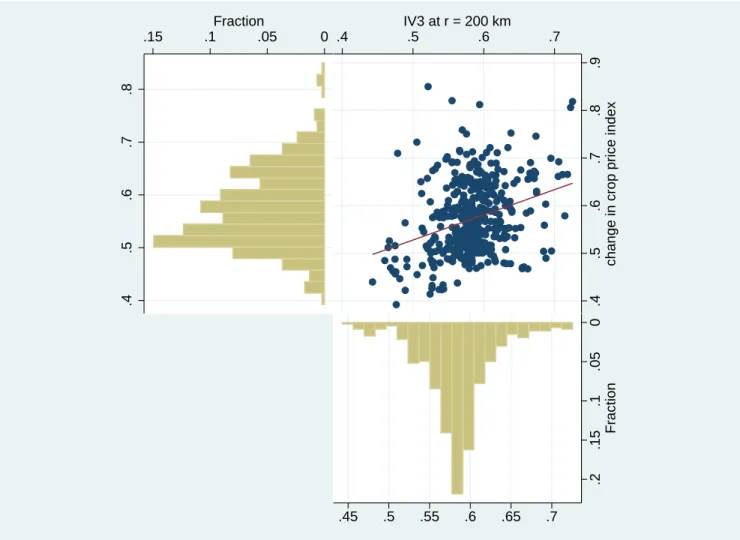
,j are not all equal, IV 3 ^r _d again essentially collapses to a constant. Figure 1 illustrates the considerable variation in P

j s _d,j ∆p _{ST AT E}

_,j across the 462 sample districts (CV = 0.130), the obviously

more limited variation in IV 3 ²⁰⁰ _d (CV = 0.073), and the regression of the former variable on

the latter–i.e., my first-stage. The adjusted R ² s of the first-stage regressions using IV 1 _d ,

IV 2 _d , IV 3 ¹⁰⁰ _d , and IV 3 ²⁰⁰ _d are, respectively, 0.788, 0.121, 0.103, and 0.091.

3.5 Inference

As already alluded to, the error term ε _d is likely to be correlated across neighboring districts, if only because geographically proximate regions experience similar productivity shocks over time. I use a nonparametric covariance matrix estimator or spatial HAC (Conley, 1999) to account for heteroskedasticity and spatial dependence. A familiar alternative to the spatial HAC is the clustered covariance estimator. But clustering standard errors by state or region assumes independence of errors across state or regional boundaries, a serious lacuna given the large fraction of districts bordering an adjacent state. ²⁵

Bester et al. (2011) show that the asymptotic normal distribution, typically used to obtain critical values for inference in HAC estimation, is a poor approximation in finite samples. I thus follow their suggestion of bootstrapping the distribution of the relevant test-statistics. For this reason, inference should be guided by p-values rather than standard errors alone, although I will follow convention and report both. In particular, bootstrapped p-values are much less sensitive than standard errors to choice of the tuning or bandwidth parameter (i.e., the degree of kernel smoothing). ²⁶

Both numerator, ∆w _d = w _d,09 − w _d,04 , and denominator, ψ _d , of the dependent variable in equation (8) are district-level summary statistics derived from micro-data. This gives rise to a particular form of heteroskedasticity and renders least-squares estimation inefficient.

The standard solution is to use weighted least-squares, taking the inverse of the estimated sampling variances as weights. While the sampling variance of ∆w _d is σ ² (w _d,09 )+ σ ² (w _d,04 ) (see above), there is no equally straightforward ‘plug-in’ estimate of the sampling variance of ψ _d . I, therefore, bootstrap this variance as well by drawing 1000 random samples of individuals from each district’s original sample and computing ψ _d repeatedly. From these

25

Also note that with only a single (five-year difference) observation per district, serial correlation is not an issue in my set-up.

26

Bandwidth here is the distance cutoff, in degrees of lat/long, beyond which spatial dependence is assumed

to die out. Based on simulation evidence from Bester et al. (2011), I choose a bandwidth of 16; i.e., given

the area of my ‘sampling region’ (the 18 major states of India), this choice should yield minimal test-size

distortion across a range of possible spatial correlations. I find these p-values to be highly robust to

bandwidth deviations of at least ±4.

two components, then, I obtain the sampling variance of ∆w _d /ψ _d using the delta-method. ²⁷

3.6 Estimation results

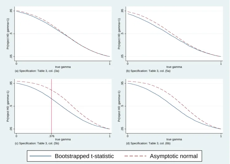
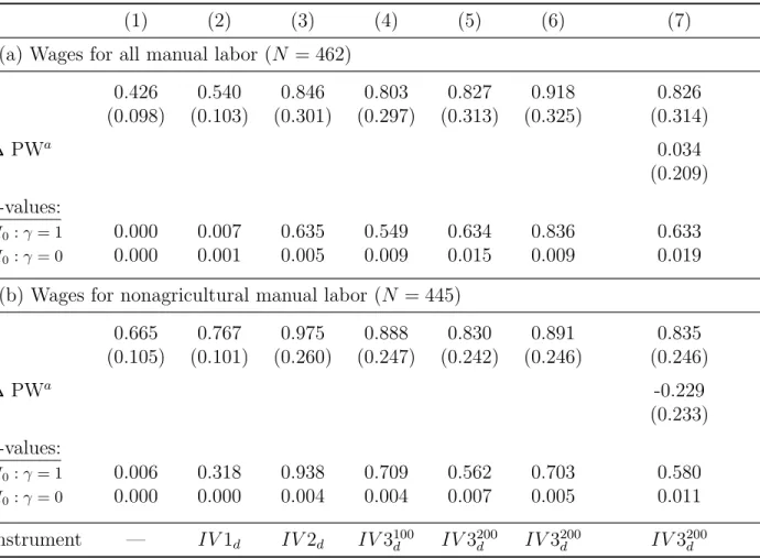
Estimates of γ based on equation (8) are reported in Table 3. Across columns 1-5 of panel (a), identifying assumptions become progressively less restrictive. Thus, column 1 estimates are by ordinary (weighted) least squares, column 2 uses IV 1 d as an instrument, column 3 uses IV 2 _d , column 4 uses IV 3 ¹⁰⁰ _d , and column 5 uses IV 3 ²⁰⁰ _d . While a comparison of the first two columns suggests that measurement error in crop shares leads to a modicum of attenuation bias, even the column 2 estimate is well below unity as indicated by the p-values from the bootstrapped-based t -test of H ₀ : γ = 1. ²⁸ Relaxing the assumption of no measurement error or simultaneity bias in price changes in columns 3-5 delivers a γ b much closer to unity, albeit one much less precisely estimated. The specifications in columns 4 and 5, however, which allow shocks to be correlated across state borders, do not give much different results from that of column 3, which ignores such correlation.

None of the p-values for H ₀ : γ = 1 in col. 3-5 are anywhere near rejection levels, evidence in favor of my baseline specific-factors model. But how powerful is this test? Clearly, this depends on the specific alternative under consideration. For instance, power will be low against an otherwise identical model that ignores income effects in the demand for services;

the implied wage-price elasticities are simply too similar to distinguish these models (compare cols. 1 and 3 of Table 1). To bring this point home, I reestimate the column 5 specification replacing ∆w _d /ψ _d with ∆w _d /ψ ^SR _d on the left-hand side and with regression weights altered accordingly. Although the resulting estimate of γ, reported in column 6, is even closer to one, it is also very close to its counterpart in column 5. Consequently, it is difficult to say which of these versions of the specific factors model fits the data better on average.

27

Although this procedure ignores correlation between numerator and denominator arising from the fact that these two statistics are calculated from partially overlapping samples of the same underlying micro-data, it should serve adequately as a first approximation.

28

The p-value is the proportion of times the bootstrapped, re-centered, t-statistic of Bester et al. (2011)

exceeds the conventional t-statistic for the null in question computed for the original sample. I use 10,000

bootstrap replications.

Power is higher against starker alternatives, such as that rural wages do not respond at all to agricultural prices. More precisely, I can use the bootstrapped t-distribution to answer the question: How likely would I have been to reject H ₀ : γ = 1 had the true γ been at or very near zero? Panels (a) and (b) of Figure 2 plot empirical power functions over the range of alternatives γ ∈ [0, 1] for the specifications in column 3 and 5, respectively. (Alongside are the corresponding power functions based on the standard normal test-statistic; consistent with Bester et al., 2011, the asymptotic approximation usually leads to over-rejection.) These bootstrap-based power functions indicate that at a true γ of zero, H 0 : γ = 1 would be rejected with 95% certainty in the column 3 specification, and with closer to 90% certainty in the column 5 specification. In this sense, then, power is reasonably good.

In sum, the evidence does not support the view that rural wages are unresponsive to agricultural price changes over a half-decade period. Moreover, the magnitude of the wage responses are consistent with at least one version of the specific factors model. Next, I assess how this model fares against a particular alternative, that of segmented labor markets.

3.7 Test of sectoral labor mobility

To test perfect intersectoral mobility of labor, I use the same procedure described above to construct log-wage district fixed effects for the 2004-05 and 2009-10 NSS-EUS rounds, except in this case using only wage data for nonagricultural jobs. The dependent variable in panel (b) of Table 3 is thus the time difference of these district fixed effects scaled by ψ _d . Relative to the previous analysis, 17 districts are missing the dependent variable because of lack of data on nonagricultural wage jobs and are thus dropped.

The estimates in columns 1-5 of panel (b) do not differ much from their counterparts

in panel (a), nor can I reject H ₀ : γ = 1 in the specifications with the least restrictive

identifying assumptions. While this non-rejection suggests that perfect mobility of manual

labor between agriculture and non-agriculture is a tolerable approximation for rural India,

the issue of power is again salient.

Recall that, under the alternative hypothesis, γ = ϕ/ψ, which is the ratio of the wage- price elasticity implied by segmented labor markets to that implied by unsegmented markets.

As seen in Table 1, γ averages 0.376 if income effects on the demand for services are operative and zero otherwise. What is the likelihood that I would have detected a deviation away from the null (towards zero) as large as γ = 0.376? Panel (c) of Figure 2 shows the power function for γ based on the column 5 specification, indicating around a two-thirds chance of rejecting H 0 : γ = 1 at γ = 0.376. In other words, the wage-price elasticities implied by the two alternative models are not sufficiently far apart to be distinguishable with near certainty in my data.

By contrast, if the demand for services was unresponsive to changes in income induced by higher agricultural prices over the five-year period in question (for reasons discussed at the end of section 2.1), then ψ ^SR is the relevant null elasticity. Reestimating the column 5 specification with ∆w _d /ψ _d ^SR as the dependent variable then leads to the b γ reported in column 6 and the corresponding power function in panel (d) of Figure 2. The upshot is that the alternative of interest in this case is γ = φ ^SR /ψ ^SR = 0, against which my test has high power (a 95% probability of rejection). Thus, provided that these income effects indeed did not materialize, my data allow me to finely discriminate a model of perfect intersectoral labor mobility from one of segmented markets.

3.8 Robustness: NREGA

India’s National Employment Rural Guarantee Act (NREGA), passed in 2005, provides ev-

ery rural household with 100 days of manual labor at a state-level minimum wage, which

is typically above the market wage. Phased in nationally beginning in 2006, NREGA, by

official counts, provided employment to 53 million households in 2010-11 over and above

existing public works programs. Imbert and Papp (2012), using NSS-EUS data and ex-

ploiting the gradual phase-in of the program, find that NREGA increased overall public

works employment while (modestly) raising private-sector wages in rural India. Since these

labor market changes were contemporaneous with rising food prices, they are worth taking seriously as possible confounding factors. Given my estimation strategy, however, NREGA will only affect the results insofar as the local expansion of the program was systematically related to the change in the agricultural price index or, rather, to the instrumental variable for this change.

Based on 7-day employment recall information in the NSS-EUS, I compute the population weighted mean of the fraction of days per week spent in public works employment (both NREGA and other) for rounds 61 and 66. ²⁹ Including the 2004-09 change in this public works employment variable (∆P W ) in regression (8) results in no appreciable changes in my estimates of γ (compare cols. 5 and 7 of Table 3). Of course, the coefficient on ∆P W does not necessarily reflect the causal impact of NREGA or any other public works employment program in India on rural wages; this specification merely serves as a robustness check.

4 Food Prices and Welfare

4.1 Welfare elasticities

Now consider a rural household embedded within the economy sketched out in Section 2.

It has an endowment of farmland and of manual labor that it can supply to its own farm (insofar as it has land) or to other farms, or to firms in the services or manufacturing sectors. Household income is simply y in equation (5) with aggregate endowments replaced by household endowments. Indirect utility is a function of this income and of prices, P M , P _S , and P _j , j = 1, ..., c. Following the conventional derivation, the percent change in

29

This is essentially the same variable considered by Imbert and Papp (2012). Across districts, the mean

days per week of public-works employment reported in 2004-05 was 0.0022, increasing to a still rather

minuscule 0.0144 days per week in 2009-10. Note, however, that NREGA employment is concentrated in

the agricultural off-season.

money-metric utility m is

m b = λ _Π Π b _A + λ _W W c − ν _S P b _S − X

j

ν _j P b _j (12)

where λ Π and λ W represent, respectively, the proportion of household income derived from owned land and manual labor and ν _j and ν _S are, respectively, the crop j and services shares of total consumption expenditures. Note that, while the last term in equation (12) is standard in the literature, the penultimate term is typically overlooked (Porto, 2006, is a notable exception).

To see how equation (12) accounts for the position of the household in the labor market, consider the special case where λ = λ _Π = 1 − λ _W and focus only on the income-side compo- nents of m, namely b λ Π b A + (1 − λ)c W . For a landless household, a net seller of labor, λ = 0 and the income effect is just W c (wage increases are unambiguously good), whereas for a pure rentier household, a net buyer of labor, λ = 1 and the income effect is Π b _A = ( P b _A −α _L c W )/α _K (wage increases are unambiguously bad). For a household with 0 < λ < 1, the income ef- fect of higher wages induced by higher food prices is positive (negative) so long as λ, the household’s land income share, is less (greater) than α _K /(α _L + α _K ), the land income share for the economy as a whole.

Substituting (1), (3), and (4), into (12), leads to

m b = X

j

(Ωs _j − ν _j ) P b _j (13)

where Ω = λ _Π (1 − α _L ψ )/α _K + ψλ _W − δν _S .

The term Ωs _j − ν _j is similar to Deaton’s (1989) well-known net consumption ratio (revenue

minus expenditures on crop j divided by total consumption expenditures) except that, un-

like Deaton’s partial equilibrium result, it fully accounts for the changes in factor income

induced by a given price change, as well as for changes in the price of nontradables. To summarize, the price elasticity of money-metric utility varies across households according to: (1) consumption shares, ν _j , including that of services, ν _S ; (2) income shares due to land (λ _Π ) and manual labor (λ _W ); and (3) sectoral labor shares, the β _j (through ψ and δ), for the district, or for the labor market more generally.

At a theoretical level, the welfare implications of a food price change look quite different when labor markets are effectively segmented. ³⁰ In particular, the counterpart to equation (13) has

Ω ⁰ = λ _A α L + α K

+ ϕλ _{N A} − δ ⁰ ν _S , (14)

where λ _A is the share of income derived from agriculture (both from land and manual labor) and λ _{N A} is the share of income derived from nonagricultural manual labor. Here, obviously, the sector in which the household supplies its manual labor matters. Inasmuch as ϕ < ψ < 1/(α _L + α _K ), landless households working in agriculture stand to gain more from higher food prices than those working outside of agriculture.

In what follows, I consider the distributional consequences of a uniform percentage in- crease in all agricultural commodity prices relative to the price of manufactures, the nu- meraire. According to equation (12), the elasticity of money-metric utility or household welfare with respect to this price is simply = Ω − ν _A , where ν _A is the expenditure share of agricultural goods (essentially the food share); in the counterfactual segmented labor markets scenario, ⁰ = Ω ⁰ − ν _A .

4.2 Baseline results

Drawing on a sample of around 61,000 rural households in 472 districts of the 18 major states from the nationally representative consumer expenditure survey (CES) collected as part of

30

Artuc et al. (2010) make a similar point in the context of trade shocks using a dynamic model of costly

intersectoral labor mobility. Perfectly segmented labor markets can be viewed as an extreme case, retaining

the analytical convenience of a static model.

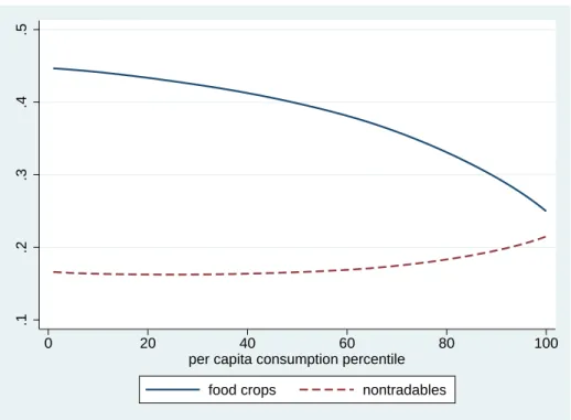
the 2004-05 NSS round 61, I obtain the expenditure shares ν _A and ν _S , along with the baseline welfare (per capita expenditure) level, for each household. Figure 3 plots these shares by per capita consumption percentiles, showing, as might be expected, opposite patterns for food and nontradables (services). ³¹

In addition to the parameters that have already been discussed, I need income shares for each household to compute Ω. Appendix B.3 describes the construction of the income components from NSS household data and Figure 4 shows how the component shares vary along the wealth distribution. Not surprisingly, manual labor earnings as a share of total income decline steadily by percentile, whereas earnings from nonmanual labor and land increase.

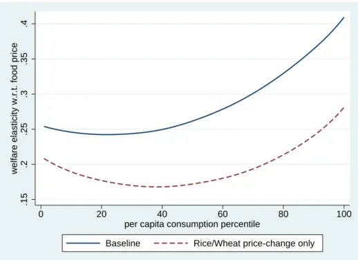
After combining all of these elements, I plot each household’s value of against its per capita expenditure percentile in 2004-05 to obtain the solid curve in Figure 5. The salient feature of this welfare elasticity profile is that it is everywhere positive. Thus, rural Indian households, both rich and poor, would benefit from higher food prices. But the profile is also increasing in household wealth, paralleling the pattern seen in the proportion of income derived from land (cf., Figure 4). So, while the welfare gain to the poorest is 0.25 percent for every one percent increase in the agricultural price index, the welfare gain to the richest is around 0.4 percent. ³²

How important are assumptions regarding intersectoral labor mobility? The lower dashed curve in Figure 5, which plots ⁰ by percentile, provides the answer. In moving to a segmented labor market, roughly a third of the gains to the very poorest households of higher agricul- tural prices are wiped away, whereas the structure of labor markets hardly affects the welfare gains of the richest households at all. The reason for this can be gleaned from Figure 4.

31

Nontraded goods expenditure categories include: firewood and other local fuel, transport and travel, tailoring expenses, house rental and related expenses, medical treatment expenses, education expenses, remittances and gifts, recreation and leisure expenses, and taxes and fees.

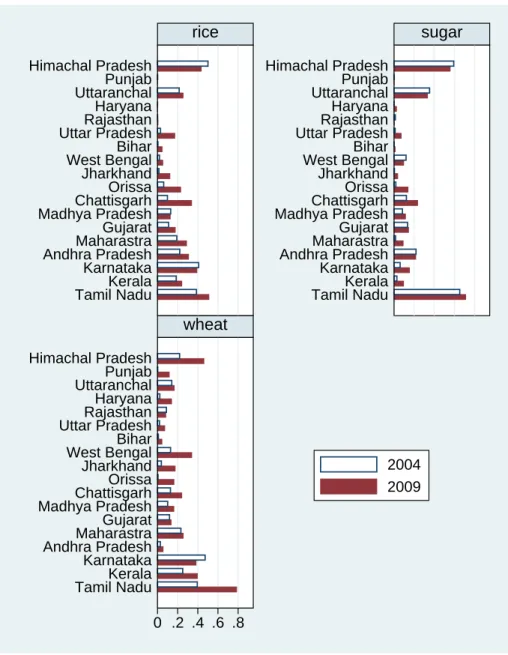
32

Results are qualitatively similar if I restrict price changes to rice and wheat, the dominant foodgrains

of India. In this case,

= Ωs

− ν

, where s

and ν

are the shares of rice and wheat in

production and consumption, respectively. Appendix Figure C.1 shows that the benefits from higher prices

are not quite as great when the increases are confined to rice and wheat and, in particular, are substantially

less advantageous to the wealthy.

The share of income from nonagricultural manual labor falls from nearly 30 percent among the poorest to only around 10 percent among the richest. But, in the segmented model, the wage paid to such labor is much less responsive to food prices than in the model with perfect intersectoral mobility. In short, ruling out labor market segmentation empirically does have consequences for how we think about the distributional effects of food price increases.

4.3 Public Distribution System

Assessing the role of the PDS in buffering price shocks provides a useful comparator as well as being of interest in its own right. Under the PDS, eligible households (generally, those below the poverty line) can purchase fixed rations of either rice, wheat, or sugar in “Fair Price Shops” at below-market (but non-zero) prices. If PDS prices rise at the same rate as non-PDS prices, then the above formula for applies. However, insofar as PDS prices rise more slowly than non-PDS prices, or do not rise at all, we need to adjust by

_{P DS} = + X

j∈C

θ _j ν _{j,P DS} (15)

where θ _j = 1 − ^∆p _∆p

j

and ν _{j,P DS} is the expenditure shares for PDS purchases of commodity j evaluated at the PDS price. Thus, to take the extreme case, if all PDS prices stay fixed while market prices rise, then instead of ν _A in the calculation of , one would use the food share net of the PDS expenditure share. To get θ _j , I take the state mean unit values from the NSS-CES for the respective commodity-types (PDS or non-PDS) in each successive round (61st and 66th). Thus, my estimate of θ _j is the ratio of percentage changes between 2004-05 and 2009-10 of state mean unit values for PDS and non-PDS purchases of commodity j.

Median values of θ _j for rice, wheat, and sugar across the 18 major states are all close to unity, which means that PDS prices were indeed quite stable over this five-year period.

The proportion of rice, wheat, and sugar consumption accounted for by the PDS generally

increased between 2004-05 and 2009-10 (Appendix Figure C.2). No doubt, this reflects the

response of government, both central and state, to the food-price crisis of 2007-08, as PDS coverage was expanded (Khera, 2011), though take-up of the existing program may have also increased. Since 2004-05 is the base year for the welfare analysis, I initially compute ν _{j,P DS} from NSS61-CES data to reflect PDS coverage circa 2004-05. However, to address PDS coverage expansion, I also calculate for each PDS commodity j and decile of per-capita expenditures q within each state s the ratio R _j,s,q of average PDS expenditures in 2009 to average PDS expenditures in 2004. Adjusting for 2009-10 PDS coverage is, then, just a matter of multiplying ν j,P DS in equation (15) by the R j,s,q corresponding to that household’s state and decile. ³³

The quantitative implications of these adjustments are shown in Figure 5. PDS coverage circa 2004-05 leads to a substantial “improvement” in the welfare elasticity for the poorest two or three deciles. When higher 2009-10 PDS coverage is factored in, the elasticity profile shifts up again ever so slightly, but only for the bottom two deciles. Although the PDS evidently plays a significant role in protecting the welfare of the rural poor, even the distributional effects of this giant safety net scheme are dwarfed by those of the rural wage channel, as we will see next.

4.4 General versus partial equilibrium

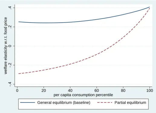
Partial equilibrium welfare analysis assumes that ψ = δ = 0 so that, from equation (13), Ω = λ Π /α K − ν A . Since λ Π /α K is equivalent to the ratio of crop revenue to total consumption, ³⁴ Ω−ν _A is just the net consumption ratio, Deaton’s (1989) justly celebrated workhorse. Figure 6 compares the partial equilibrium welfare elasticity profile (dashed curve) to the general equilibrium case already discussed. In partial equilibrium, the poorest rural households in India would experience a welfare loss of around 0.3 percent for a 1 percent uniform increase in agricultural prices. But the distributional gradient is very steep, so much so that the top

33

To be clear, while NSS66-CES provides household-level data on PDS consumption from 2009-10, these are not the same households as in the NSS61-CES of 2004-05. Thus, to keep 2004 as the base-year, I need to impute to this latter sample of households what their 2009 PDS coverage would have been.

34

This is because λ

/α

= Π

K

/yα

= P

Y

/C, where C is household consumption.

30 percent of rural households would gain from the price increase, and those households at the very top would gain by more, in percentage terms, than the poorest households would lose.

Among the poor, the chasm between partial and general equilibrium welfare elasticities is enormous (note the difference in scale vis ` a vis Figure 5). Income from land, which incorporates the direct return to higher crop prices, is concentrated in top half of the wealth distribution in rural India, whereas income from manual labor dominates for the bottom half. So, it is the poor in particular whose welfare is most sensitive to changes in wages for manual labor. In general equilibrium, improved terms of trade for the agricultural sector is like the proverbial rising tide that lifts all boats; every rural income group comes out ahead, albeit through different channels.

5 Conclusions

In reaction to the food price spike of 2007-08, the Government of India imposed export bans on certain major crops. Such efforts to restrain consumer prices can have the unfortunate side-effect of restraining producer prices as well. My analysis shows that, in the face of higher agricultural commodity prices, a stand-alone export ban, or any policy that mimics its effects, would reduce welfare for the vast bulk of India’s population. Moreover, it is precisely the poorest rural households (and, hence, the poorest in India as a whole) that are most harmed by forestalling, or at least delaying, the substantial trickle-down effects of higher crop prices.

Looking over a period of unusually large and diverse agricultural commodity price in-

creases, I find a highly elastic nominal wage response in rural areas of India, with ample

spillover effects on nonagricultural wages as well. Consequently, partial equilibrium analysis,

which assumes fixed wages, would provide a highly misleading picture of the distributional

impacts of food price shocks among India’s vast rural population.

To be sure, the story may be quite different in metropolitan India, where the poor, arguably, benefit little from rising rural wages. ³⁵ Even though not much more than a quarter of India’s population resides in cities, urban constituencies are obviously more concentrated than rural ones and, hence, from a political-economy standpoint, are likely to be more pivotal in shaping government policy on such matters as food security.

Finally, this paper speaks to the broader debate on the link between trade and poverty. ³⁶ Consistent with the WTO’s Doha agenda, my results imply that lowering barriers to trade in agricultural goods on the part of developed countries, if only by improving the lot of the rural poor in India, can make a significant dent in global poverty.

35

A full analysis of rural-urban labor market linkages is beyond the scope the present paper, but is an important topic for future research.

36

The evidence on the impact of India’s own tariff reform during the 1990s is mixed. Topalova’s (2010)

ex-post analysis finds that rural poverty rose and agricultural wages fell in districts exposed to larger tariff

reductions, although the main agricultural commodities are assumed to be nontradable over the reform

period. By contrast, Marchand (2012) finds a negative relationship between unskilled wages in rural areas and

industry-specific tariff rates, including those in agriculture, and an ex-ante analysis of household consumption

suggests that the fall in trade barriers during the 1990s would have reduced rural poverty in India.

References

[1] Artuc, E., S. Chaudhuri, and J. McLaren. 2010. “Trade shocks and labor adjustment:

A structural empirical approach,” American Economic Review, 100(3):1008-45.

[2] Atkin, D. 2011. “Trade, Tastes and Nutrition in India,” unpublished manuscript, Yale University.

[3] Boyce, J. and M. Ravallion. 1991. “A dynamic econometric model of agricultural wage determination in Bangladesh,” Oxford Bulletin of Economics and Statistics, 53(4):361- 76.

[4] Bester, C. A., T. Conley, C. Hansen, and T. Vogelsang. 2011. “Fixed-b asymptotics for spatially dependent robust nonparametric covariance matrix estimators,” unpublished manuscript, University of Chicago.

[5] Conley, T. 1999. “GMM estimation with cross sectional dependence,” Journal of Econo- metrics, 92: 1-45.

[6] Datt, G. and M. Ravallion. 1998. “Farm productivity and rural poverty in India,”

Journal of Development Studies, 34(4):62-85.

[7] Deaton, A. 1989. “Rice prices and income distribution in Thailand: A non-parametric analysis,” Economic Journal, 99:1-37.

[8] Eswaran, M., A. Kotwal, B. Ramaswami, and W. Wadhwa. 2008. “How does poverty decline? Suggestive evidence from India, 1983-1999,” unpublished manuscript, Univer- sity of British Columbia.

[9] Goldberg, P. and N. Pavcnik. 2007. “Distributional effects of globalization in developing

countries,” Journal of Economic Literature, XLV:39-82.