13 Eulerian Models

13 Eulerian Models

In a fixed, Eulerian frame of reference the temporal and spatial development of an air pollutant’s (tracer’s, in general) concentration is described by the conservation equation of mass for the tracer concentration, C (eq. 5.1d)

€

∂C

∂t + u

∂C

∂x

= Q + S _(5.1d)

Thus the total rate of change of tracer concentration (lhs 0f 5.1d) is equal to the sources (‘Q’) plus the sinks (‘S’). Apparently the sinks assume negative values in this notation. Applying Reynolds decomposition and averaging yields

€

∂C

∂ t + u

∂C

∂ x

+ ∂

∂ x

(u'

c') = Q + S _{. (5.25)}

Solution of (5.25) is the backbone of modelling air pollution dispersion in a turbulent flow. Apparently, this requires knowledge of the flow field that can be obtained from observations (using, e.g., similarity theory to get the information in the vertical) or from running a numerical model. In addition, knowledge on the turbulence characteristics is required in order to determine the turbulent flux divergence term.

It is noted here that we implicitly assume in what follows that the flow and turbulence fields are independent of the tracer concentration. This is not strictly true, if we think for example of possible radiative effects certain trace gases have, thus influencing the thermodynamics (stability!) of the flow itself.

Still, if not extreme tracer concentrations are present the assumption of independence between flow and tracer concentration usually yields considerable simplifications so that it is usually invoked. An Eulerian dispersion model, therefore, is in general constructed by adding one (or more, for different tracers) mass conservation equations to the set of conservation equations (Table 5.2) for the boundary layer flow. Solving these equations requires additional knowledge on chemical reactions between different species, which enter the source and sink terms, respectively. If these chemical reactions are fast enough as compared to the model time step, source and sink terms can ‘relatively easy’ be introduced by solving a

‘chemistry module’ at each time step by finding the increments of the tracer concentrations according to the chemical reactions among the species considered. If the chemical reactions among the species involves more complicated processes (as for example in the Ozone chemistry where a set of fast reactions among O

, NO and NO

competes with a quite extensive set of slower reactions involving a number of other species), careful consideration has to be given to the ‘time splitting’ between turbulence (flow) and chemical development of the tracer concentrations (REF  Galmarini papers).

Here we concentrate on the case of a passive tracer, i.e. it is assumed that no

chemical (or other) reaction modifies the tracer concentration and we only

describe the turbulence and transport in a (turbulent) flow. It is first investigated what simplifications can be made to (5.2) in order to obtain an analytical solution, which then would yield ‘the simplest dispersion model’ in combination with a known boundary layer flow.

13.1 First-order closure

The problem in solving (5.2) is, apparently, the flux divergence term. As has been noted in Chapter 5 for the turbulent fluxes of the flow variables, the simplest approach for the unknown

€

u'

c', i.e. the turbulent flux of tracer concentration, consists in a first-order closure. Thus the flux is modelled by

€

u'

c' = − K

∂C

∂x

^{. (13.1)}

€

K

is a second order tensor and its elements are usually referred to as ‘eddy diffusivities’. If we assume (for simplicity) that only its diagonal elements are different from zero, (5.2) reduces to

€

∂ ^C

∂ ^{t = − u}

∂ ^C

∂ ^x

+ ∂

∂ ^x

K

∂ ^C

∂ ^x





 





  + S + Q , (13.2)

where we have replaced the double subscript (in

€

K

) by a single for simplicity.

In the simplest case of constant (but not necessarily equal for different j)

€

K

, the dispersion process as described by (13.2) is called ‘Fickian’.

We first concentrate on an idealised situation for which an analytical solution to (13.2) can be found. Idealisations are: homogeneous conditions in the cross-wind direction (

€

∂ ∂ x

= 0 )

, stationarity (

€

∂ ∂ t = 0 ), no mean vertical flow (

€

u

= 0 ), no sinks (S=0) and only one constant source (Q) at x

=0. In this case (13.2) reduces to

€

u

∂ ^C

∂ ^x

= ∂

∂ ^x

K

∂ ^C

∂ ^x



  

  (13.3)

For the ‘flow variables’ we make the following approach:

u

= ( ) u

⋅ x

x





 

 

p

K

= ( ) K

^{⋅ x}

x





 

 

m

(13.4)

As boundary conditions, it is assumed

€

C → 0 for

€

x

, x

→ ∞ _(13.5a)

1

It becomes immediately clear, that we deal here with an infinite line source in the crosswind

direction , at x

=0. Thus we are considering a two-dimensional problem that is obtained first

integrating (13.2) in the crosswind direction. The result, is then strictly speaking a ‘cross-wind

integrated concentration’ (see Chapter 12).

€

C → ∞ for

€

x

+ x

= 0 _(13.5b)

€

K

∂C

∂ x

→ 0 for

€

x

→ 0, x

> 0 ^(13.5c)

For this problem the solution reads

€

C (x

, x

) = Qr

2x

(u

)

⋅ Γ ( ) s ^⋅ u

( )

x

r

( ) K

x

















s

exp − ( ) u

x

r

( ) K

x

⋅ x

x



  

 



 

 



 

 

(13.6) Here, Q is the source strength (in [kgs

m

],

€

Γ the Gamma function,

€

r = m − p + 2 and

€

s = (1 + m) / r . Solution (13.6) is valid for

€

m − p + 2 > 0. It has been devised by Roberts (1923) and is therefore called ‘Robert’s solution’. We note that the vertical distribution of mass is in this idealised case essentially given by an exponential function. Typical values for

€

m and

€

p can be determined from turbulence theory or observations. More directly,

€

s and

€

r may be estimated from tracer experiments. Table 13.1 lists some typical values for these parameters.

Table 13.1: Typical values of the parameters in the power laws for K

and u

and in the solution of the diffusion equation for a line source (from Gryning, 1981).

Parameter Neutral, Neutral Moderately Free

Smooth surface Rough surface unstable convection

p 1 1 1.1 1.33

m 0.14 0.4 0.1 0

r 0.14 1.4 1 0.67

s 1 1 1.1 1.5

13.2 Gaussian Plume Models

Before proceeding we first address an issue that sometimes causes irritation.

What is going to be presented in this section, as expressed in the title, is a

plume model – what was introduced in Chapter 12 as the simplest of the

Lagrangian approaches. And indeed the solution to be presented corresponds

to an analytical description of a plume that as similar properties as the

theoretical plume according to the Theory of Taylor (Chapter 12) – hence its

name. Since the derivation is based on the mass conservation equation and

therefore basically an Eulerian approach, Gaussian plume models are

nevertheless discussed in this chapter.

Considering the (two-dimensional) Robert’s solution for the special case of

€

m = p = 0 yields a concentration distribution that exhibits a normal (or Gaussian) shape in the vertical. This is the famous ‘Gaussian plume model’

for the two-dimensional case. We readily note that the assumptions for this solution are even more radical than those leading to Robert’s solution:

€

m = p = 0 means that both the mean wind speed and the exchange coefficient do not vary with height (see eq. 13.4)! With all these assumptions an analytical solution to (13.2) can also be found for the three-dimensional problem. Again stationarity is assumed, in addition we require that neither mean wind speed nor the exchange coefficients vary with height (

€

m = p = 0) and furthermore no diffusion in longitudinal direction (

€

K

∂C ∂x

= 0 ) with a constant point source at (0,0,H) and no sinks. With this (13,2) reduces to

€

u

∂ C

∂x

= K

∂

C

∂x

, j = 2,3 _{. (13.7)}

The boundary conditions for the three-dimensional problem are chosen as follows

€

C → 0 for

€

x

→ ±∞ and x

→ ∞ (13.8a)

€

K

∂C

∂x

→ 0 for x

→ 0 (13.8b)

As an initial condition, finally

€

C(x

= 0, x

= 0, x

= H) = Q

u

δ (x

− H ) δ (y ) (13.8c) The solution to this problem reads

€

C x (

, x

,x

) ⁼ _{2 πσ} ^Q

y

σ

u

exp − 1 2

x

σ





 





 



 

 



 

 

exp − 1 2

x

− H σ



  

 



 

 



 

  + exp − 1 2

x

+ H σ



  

 



 

 



 

 















 (13.9)

In (13.9) the ‘plume characteristics’

€

σ

and

€

σ

have been introduced according to

€

σ

= 2K

x

/ u

, (13.10)

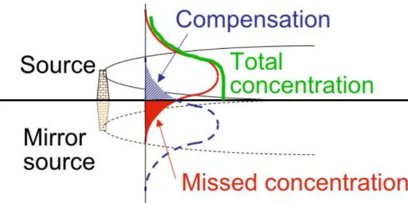
thus relating the ‘plume width’ and ‘plume depth’, respectively to the basic variables. Note that the second contribution in the rectangular parenthesis on the rhs of (13.9) is necessary due to the lower boundary condition. It corresponds to a second ‘mirrored’ source at

€

x

= −H , i.e. ‘below the ground’.

Without this mirror source a substantial part of the mass from the ‘real’ source

would be placed below the ground (Fig. 13.1) – and this is compensated for

by the corresponding mass fraction from the mirror source. Due to the fact

that a similar (though less stringent) problem occurs at the boundary layer top

(the ‘infinite’ Gaussian distribution places a fraction of the pollutant mass up to

infinite heights), sometimes, additional mirror sources are introduced by mirroring –H etc.

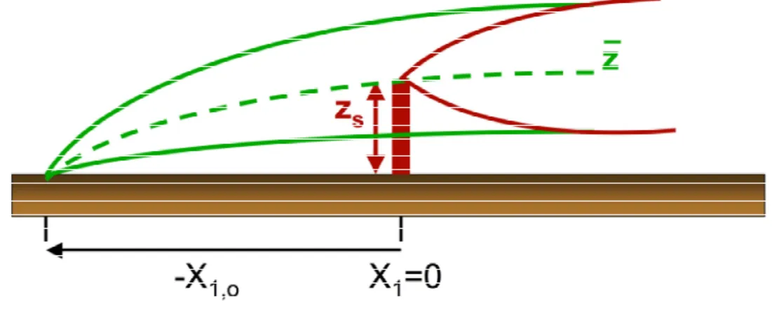
Figure 13.1 Sketch of a Gaussian plume (black solid line) and the corresponding vertical concentration distribution (red line) from a source above the ground. The ‘mirror source’ yields a ‘mirrored Gaussian plume’ (dashed black line) and the corresponding vertical concentration profile (dashed blue line). The total concentration profile is sketched as the green full line.

Despite the quite unrealistic assumptions leading to solution (13.9), Gaussian plume are widely employed due to their simplicity (analytical solution) and the relatively few required input parameters. A solution can be obtained for many sources at virtually no (cpu) costs thus making Gaussian plume models attractive for planning purposes, such as investigating for example the effect of modified emission control regulations for vehicles or domestic heating in a wider area. Having noticed the stringent assumptions leading to (13.9) an assessment on weak and stronger (if not to say: less weak) aspects of this model class is in order.

 Equation (13.10) indicates that plume width and depth grow proportional to

€

x

. Recalling the results from Taylor’s theory - and invoking Taylor’s hypothesis (

€

x

= u

⋅ t , in its simplest form) - this indicates that Gaussian plume models are certainly incorrect close to the source. Often in practical applications a fixed ‘limit’ (e.g.

€

x

> 100m ) is employed to take into account for this limitation.

 Due to the assumption of constant mean wind speed and exchange

coefficients in the vertical (what is wrong of course) Gaussian plume

models are least valuable for sources near the ground.

 The assumption of a ‘K-type’ (first order) turbulence closure relates the turbulent flux (of the tracer) to the local mean tracer concentration. In Chapter 5 (Fig. 5.3) it was shown that this assumption is particularly vulnerable in the Mixed Layer (or free convection) regimes.

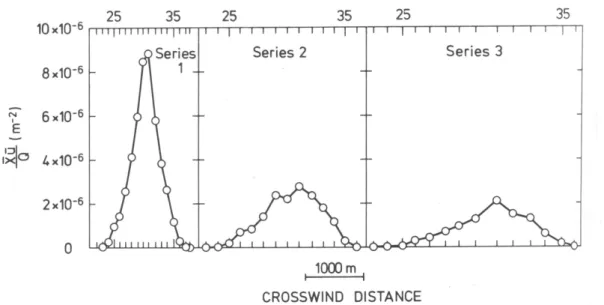
Thus, Gaussian plume models are possibly best under stable conditions and for sources not too close to the ground. Certainly their use is not advisable under convective conditions. Last but not least we note that the problem with the plume approach lies mostly in the vertical direction (due to the ‘preferred’

direction of action close to the surface). Figure 13.2 shows the tracer distribution at three different positions downwind of a source, indicating that a Gaussian distribution is not so bad to describe reality in the crosswind direction.

In general, the success of Gaussian plume models (i.e., the accuracy, to which concentrations can be estimated) depends mainly on how the ‘sigmas’

(

€

σ

and

€

σ

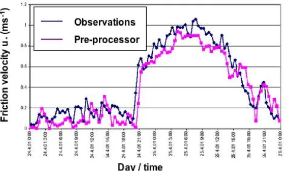
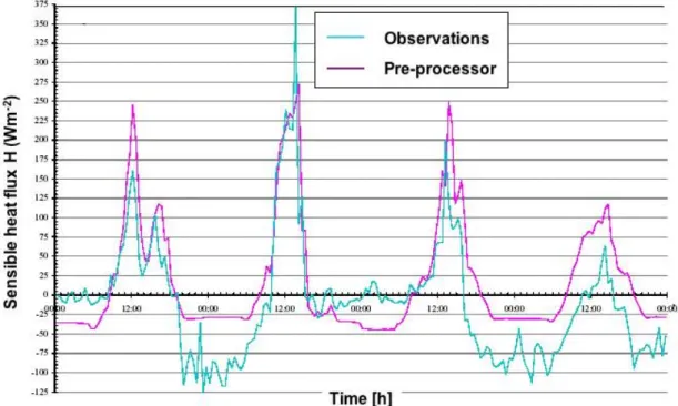
) are determined. In air pollution modelling the procedure to estimate turbulence parameters from standard meteorological data (like mean wind speed or temperature) is called a meteorological pre-processor.

Traditionally, a meteorological pre-processor would be based on so-called stability classes (Pasquill-Turner stability classes; Pasquill, 1961, Turner 1970). Based on some broad ranges of net radiation and wind speed these classes divide the stability range into classes A to F and devise some simple relations (based on tracer experiments) to estimate

€

σ

and

€

σ

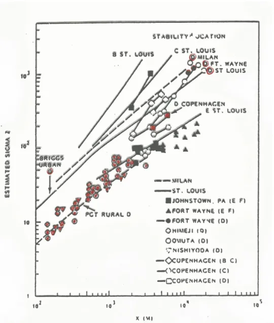
for each class as a function of distance. Figure 13.3 shows a compilation of estimates for

€

σ

from different sources. Noting the double-logarithmic scale and the wide range of results for one and the same class, indicates the accuracy that can be obtained with this type of approach.

Figure 13.2 Observed crosswind concentration distributions from a tracer experiment in Copenhagen (DK). From Gryning (1981).

A better approach for a meteorological pre-processor would be to employ

similarity relations in order to first estimate the basic turbulence variables

(such as the friction velocity, the surface heat flux or the velocity fluctuations,

€

u'

). In a second step the semi-empirical estimates for the plume characteristics under the given stability conditions (section 12.3) are then employed in order to obtain the input for solving eq. (13.9). This approach is sometimes referred to as Gaussian plume model of the new generation.

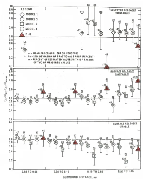
Figure 13.4 shows the degree of improvement that can be achieved with this approach as compared to the traditional Pasquill-Turner (PG) type of model.

At the same time Fig. 13.4 also reveals the limitations that even the new generation models still have in terms of accuracy: if most of the concentrations are predicted within a factor of two of the observations, this is already a ‘good’ Gaussian plume model.

Figure 13.3: Compilation of various observations of plume depth (

€

σ

) over urban

areas. City names are indicated and the associated letters (A, B, …)

refer to Pasquill-Turner stability classes. Marked with red are (as an

example) all results for class D. From Ramsdell et al. (1982).

Figure 13.4: Comparison of model performance between different Gaussian plume models (model 1 to 4) of the ‘new generation’ and a Pasquill-Turner type of model (‘P-G’). Shown is the ratio of modelled to observed surface concentration as a function of downwind distance from the source. Statistical measures as defined in the inlet. Each panel depicts a different type of source. P-G model is coloured red. From Irwin (1983).

13.3 Solution of van Ulden

In this section we consider another solution for the problem (13.3), i.e. an

idealised, stationary two-dimensional case with mean vertical velocity

vanishing and no sinks. For this situation van Ulden (1978) introduces a way,

how to incorporate surface layer similarity (MOST) in order to obtain a

physically more reliable result. This solution to (13.3) can be written (van Ulden (1978)

€

C

Q = A

z ⋅ < u > exp − Bz z



  

 



 

 



 

  ^(13.11)

Here, as in Robert’s solution

€

r = m − p + 2, and the velocity and ‘K’-profiles were approximated similarly to (13.4) according to

€

u

= ( ) u

⋅ x

K

= ( ) K

⋅ x

(13.12)

In (13.11) an ‘average plume height’,

€

z , is used that is defined as a weighted average of the mean concentration

€

z = C x

dx

0

∞

∫ C dx

0

∞

∫ (13.13)

Similarly, a weighted average of the mean wind speed,

€

< u > , is used (the brackets being introduced to denote the concentration weighing)

€

< u >= u C dz

0

∞

∫ C dz

0

∞

∫ . (13.14)

Finally the auxiliary functions A and B are

€

A = r Γ 2 r



  

  Γ 1 r



  

 



  

 

2

(13.15)

€

B = Γ 2 r



  

  Γ 1 r



  

  (13.16)

Fist of all, we note that the solution is qualitatively similar to Robert’s solution in that the vertical concentration profile is essentially proportional to

€

exp { } −x

^. The concentration evolution in along-wind direction is ‘hidden’ in

€

z x ( )

^{. To}

investigate this property we start from the definition (13.3) and consider the total differential

€

dz = 1 C dx

0

∞

∫

∂

∂ x

( C x

dx

0

∞

∫ )dx

−

C x

dx

0

∞

∫ ( C dx

0

∞

∫ )

∂

∂ x

( C dx

0

∞

∫ )dx

(13.17)

Thus

€

dz

dx

= 1 C dx

0

∞

∫

∂

∂ x

( C x

dx

0

∞

∫ ) − z ∂

∂ x

( C dx

0

∞

∫ )



  

  (13.18)

Due to the fact that x

and x

are independent the derivatives and integrations can be interchanged

€

dz

dx

= 1 C dx

0

∞

∫

∂

∂ x

(C x

) − z ∂ C

∂ x



  

 

0

∞

∫ dx

(13.19)

and hence

€

dz

dx

= 1 C dx

0

∞

∫

(x

− z ) ∂ C

∂ x

dx

0

∞

∫ . (13.20)

Using the original differential equation (13.3), the potential profiles (13.12) and also the final solution (13.11), it is straightforward to find

€

dz

dx

= rB

( (K

)

(u

)

) ⋅ z

(13.21) Equation (3.21), in turn, can be brought to the following form

€

dz

dx

= K

( ) pz

u

( ) pz ^⋅ ( ) ^{pz , (13.22)}

where

€

p = [ ] rB

^(13.23)

(again having used the definitions (13.12)). In the form (13.22) the derivative the weighted mean plume height with respect to

€

x

is only dependent on the parameter

€

r . However, abbreviation

€

p is very insensitive to

€

r . For typical values of

€

r in the Surface Layer (1.3 to 2.1)

€

p varies between 1.54 and 1.57.

Thus p=1.55 may serve as a suitable choice.

Inspecting (13.22) shows that the profiles of the mean wind speed and the exchange coefficient are required – and here is where MOST is introduced.

For the exchange coefficient, van Ulden adopts the (usual) assumption that the exchange coefficient for a tracer is equal to that for sensible heat

€

K

. Thus using its definition (

€

K

= −∂θ ∂x

) and the non-dimensional gradient of potential temperature (4.25) we have

€

K

= kx

u

/ Φ

(x

/ L) (13.24)

For the wind speed profile Surface Layer similarity predicts

€

u

( ) z ^{= u} _k

^{ln x} _z

o



  

  − Ψ

x

L



  

 



  

  (4.20)

Thus replacing the arguments in (13.24) and (4.20) [ x

→ pz ] (13.22)

becomes

€

dz

dx

= k

ln pz z



  

  − Ψ

pz L



  

 



  

  ⋅ Φ

pz L



  

 

(13.25)

For stable conditions, both

€

Ψ

= −β x

/ L and

€

Φ

= 1 + β

x

/ L are linear and (13.25) can be integrated using separation of variables. This yields

€

x

(z ) , rather than the desired

€

z (x

) :

€

x

+ x

= z k ln( cz

z

) + c β ( pz

3L )(1 + β

^pz 2L ) + ( β

4 − β

6 ) pz

L



  

  , (13.26) where c=0.6, At least, (13.26) can be used in an iterative fashion to the desired

€

z (x

) . For unstable conditions, integrating (13.25) is a little more involved and van Ulden (1978) only gives an approximate solution.

The meaning of

€

x

is primarily that of an integration constant. However, it can be used to introduce a source height different from zero. Figure 13.5 shows the situation with an imaginary (surface) source at

€

x

= −x

, chosen such that at

€

x

= 0 the mean plume height reaches

€

z = z

i.e. the desired source height. Determination of

€

x

is straightforward by solving (13.25) for

€

x

under these conditions.

Figure 13.5 Meaning of the integration constant

€

x

in the dispersion modelling approach of van Ulden (1978) for the Surface Layer.

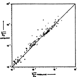
Figure 13.6 shows a comparison between observed and modelled crosswind

integrated concentrations from van Ulden (1978). As can be seen the

correspondence is rather fortunate (although the logarithmic scale should be

noted!). Even with this relatively sophisticated approach that includes surface

layer theory quite a few ‘points’ are outside the ‘factor of two’ range. Thus this

result shows the quality one can obtain for dispersion calculations with the

plume model approach – even under relatively ideal conditions.

Figure 13.6: Comparison of computed (vertical axis) and measured (horizontal axis) crosswind-integrated surface concentrations normalized by the source strength. Simulations with the model of van Ulden (1978) for quasi- ideal observations (tracer experiments in horizontally homogeneous environments). From van Ulden (1978).

13.4 Hybrid models

For practical applications it was noted above that dispersion models need primarily to be fast (computationally efficient). Thus whenever possible the simplest (Gaussian plume) model approach would be chosen if a large number of sources (and/or cases) are to be modelled. However, we have also found that for certain conditions (e.g. stability, source height) the Gaussian model would be particularly bad (e.g., convective stratification). Thus, hybrid approaches have been proposed that consider for each scaling regime (Chapter 4) the most appropriate of the simple (analytical) dispersion modelling approaches. Gryning et al. (1987) thereby use the scaling regimes as introduced in Chapter 4 (Fig. 4.4). For the Surface Layer they suggest van Ulden’s (1978) solution. Due to the lack of better knowledge they suggest employing Gaussian plume models for the Local Scaling and Z-less Scaling Layers as well as for the Near-Neutral Upper Layer. For the Mixed Layer they propose an empirical model originally provided by Briggs (1985)

€

χ

= 0.9X

Z

Z

+ 0.4X

Z

[ ]

⁺

1

1+ 3X

Z

+ 50X

[ ] ^(13.27)

where

€

χ

= C

z

u

/ Q is a non-dimensional crosswind integrated surface concentration,

€

X = (w

/ z

) ( x

/ u

) is the non-dimensional distance, and

Z

= z

/ z

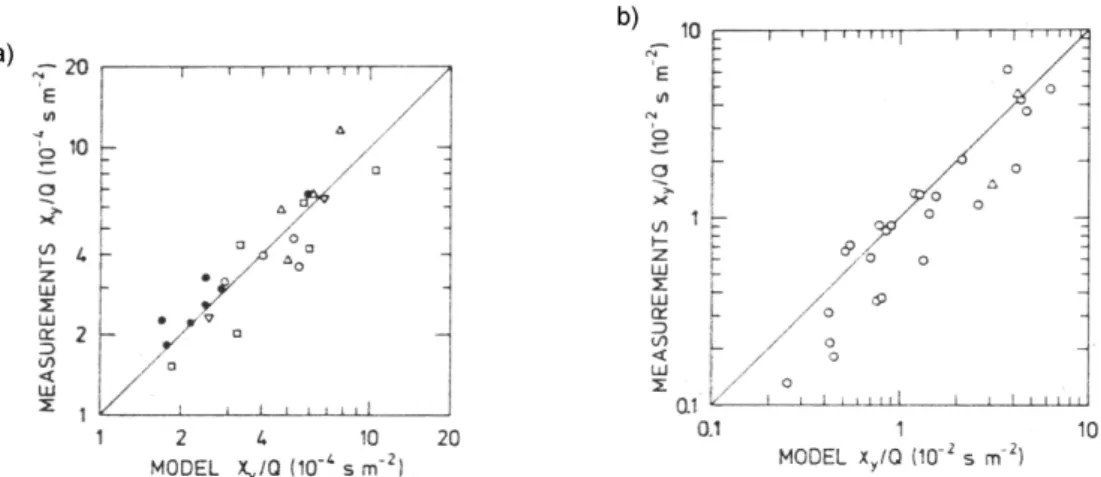
the non-dimensional source height. Figure 13.7 shows modelled

and measured surface concentrations for some carefully selected tracer

experiments. For ideally flat horizontally homogeneous conditions under

convective conditions thus the ‘reproducibility’ is quite good. Under stable conditions, however some data show a pronounced overestimation – most likely due to the fact that under stable conditions sometimes the turbulence brakes down (this would effectively then correspond to the (Intermittency scaling Regime, Fig. 4.4) and hence ‘turbulence based’ dispersion models do not apply in principle (Gryning 1999).

Figure 13.7 comparison of observed vs. modelled cross-wind integrated surface concentrations based on the hybrid dispersion model of Gryning et al.

(1987), a) unstable conditions , b) stable conditions (from Gryning et al.

1987).

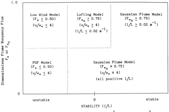
Similarly, Hanna and Chang (1993) have devised the Hybrid Plume Dispersion Model (HPDM), which is also based on a distinction in different regimes, but in their case in the stability-plume buoyancy flux space (Fig. 13.

8). The dimensionless plume buoyancy flux is defined for convective and neutral conditions, respectively

€

convective : F

= F / u

w

z

neutral : F

= Fu

u

z

^(13.28) where the plume buoyancy flux is given by

€

F = g

T / w

R

Δ T

(13.29)

with

€

w

being the stack plume exit speed,

€

R

the stack’s radius and

€

ΔT

the emissions excess temperature. Thus this modelling approach takes into account the so-called plume rise, i.e. the fact that a warm exhaust gas first rises due to its excess buoyancy before the ‘classical’ plume dispersion takes over

.

2

Some fundamentals about plume rise will be discussed in Chapter 15.

Figure 13.8 Phase space illustration for the hybrid dispersion model of Hanna and Chang (1993). From Hanna and Chang (1993).

In addition to the hybrid dispersion model, the paper of Hanna and Chang (1993) includes a complete Meteorological Pre-Processor (MPP). With this we denote a ‘set of relations’ (equations), from which the necessary turbulence variables (e.g.,

€

u

, w

σ

, z

) can be estimated if only standard meteorological observations (such as

€

u

, Q

, T ) are available. A MPP is based on similarity relations (MOST, in their case) wherever possible and approximations based on suitable statistical approaches wherever the available standard observations do not yield enough information. Clearly, such a MPP may be devised for application in specific situations, as for example dispersion

 over flat horizontally homogeneous areas

 over urban areas (e.g. Rotach 1997)

 in complex terrain (e.g., Penelon et al. 2001)

 for special stability conditions (e.g., Johansson 1997)

The more complex the boundary layer structure (see Chapter 8) the larger will

be the partition in the MPP that is based on empirical result rather than

theoretically based similarity relations. The MMP of Hanna and Chang (1993)

has especially been designed to also include effects of enhanced mechanical

mixing in urban areas. Still, Fig. 13.9 shows that it can even successfully be

applied in highly complex terrain such as the floor of a rather steep valley in

the Alps. This is mainly due to the fact that the mechanical processes relating

the mean wind speed to the turbulence variables (friction velocity, in this case)

are rather local and are not substantially modified by the nearby slopes. The

same is true for the thermally induced turbulence (surface sensible heat flux in

Fig. 13.10), except during a day with pronounced advective conditions (Föhn), during which potentially warm air is advected aloft leading to reduced surface heat fluxes, while the MPP ‘suggests’ too high fluxes due to the relatively large net radiation associated with the warm advected air and cloud-free conditions. Figure 13.10 also reveals that the stable conditions during the night are harder to predict than the daytime conditions.

Figure 13.9 Comparison of predicted (Hanna and Chang, 1993) vs. observed friction velocity during two days in April 2001. Observations in the Reuss Valley in central Switzerland (an U-shaped major valley with a valley floor of approximately 2km width. Observations with a sonic anemometer.

In general, due to the fact that MPPs are commonly to some extent based on

empirical relations, any given approach should either be used exclusively in

the environment for which it had been developed, or tested for any other

application.

Figure 13.10 Comparison of predicted (Hanna and Chang, 1993) vs. observed surface sensible heat flux during four days in April 2001. Observations as in Fig. 13.9. Note the difference between the first three days (no Föhn) and the last day (Föhn conditions).

References

Briggs GA: 1985, Analysis parameterizations of diffusion – the convective boundary layer, J

Gryning SE: 1981, ‘Elevated Source SF6 Tracer Dispersion Experiments in the Copenhagen Area’, Risø Report Risø-R-446, Risø National Laboratory, Roskilde, DK, 187 pp.

Gryning SE, Holtslag AAM, Irwin JS, Sievertsen B: 1987, Applied Dispersion modelling based on meteorological scaling parameters, Atmos Environ, 21 (1), 79-89.

Gryning SE: 1999, Some aspects of atmospheric dispersion in the stratified atmospheric boundary layer over homogeneous terrain, Boundary-Layer Meteorol, 90 (3), 479-494.

Hanna SR and Chang JC: 1993, Hybrid Plume Dispersion model (HPDM). Improvement and testing at three field sites, Atmos Environment, 27A, 1491-1508.

Irwin JS: 1983, Estimating plume dispersion – a comparison of several sigma schemes, J

Johansson PE: 1997, Comparison of meteorological pre-processors during high-latitude winter conditions, Int. J. Environment and Pollution, 8, Nos. 3-6, 574-582.

Pasquill F: 1961, The estimation of the dispersion of windborne material, Metoeol Mag, 90, 33-49.

Penelon T, Calmet I, Mironov DV: 2001, Micrometeorological simulations over a complex

terrain with SUBMESO: a model study using a novel pre-processor, Int J Environment

Roberts OFT, 1923: The theoretical scattering of smoke in a turbulent atmosphere, Proc Roy

Rotach, M.W.: 1997, 'Towards a Meteorological Preprocessor for Dispersion Models in an Urban Environment', Int. J. Environment and Pollution, 8, Nos. 3-6, 548-556.

Turner, DB: 1970, Workbook of atmospheric dispersion estimates, National Air Pollution Control Administration, Cincinnati, Ohio, HPS Pub, 999-AP-26, 88pp.

van Ulden AP: 1978, Simple estimates for vertical diffusion from sources near the ground,

Ramsdell, JV, Hanna SR and Cramer HE: 1982, Turbulent diffusion coefficients within and

above the urban domain, US Army Atmospheric Science Laboratory report, 85pp.